[

Solution of the Quantum Sherrington-Kirkpatrick Model

Abstract

We solve the $S=1/2$ infinite-range random Heisenberg Hamiltonian in the paramagnetic phase using quantum Monte Carlo and analytical techniques. We find that the spin-glass susceptibility diverges at a finite temperature $T_{g}$ which demonstrates the existence of a low-temperature ordered phase. Quantum fluctuations reduce the critical temperature and the effective Curie constant with respect to their classical values. They also give rise to a redistribution of spectral weight in the dynamic structure factor in the paramagnetic phase. As the temperature decreases the spectrum of magnetic excitations gradually splits into quasi-elastic and inelastic contributions whose weights scale as $S^{2}$ and $S$ at low temperature.

]

It is well known that the combined effects of randomness and frustration may lead to spin glass behavior in classical disordered magnets at low temperature. The most widely studied spin-glass Hamiltonian is the Sherrington-Kirkpatrick model[1]. However, only a small fraction of the vast amount of work[2] devoted to this model directly addresses the role of quantum fluctuations. In a notable early paper Bray and Moore [3] first formulated the theory of the quantum Sherrington-Kirkpatrick model and showed that it reduces exactly to an effective single site problem in imaginary time. Using a variational approach, these authors argued that a spin glass ordered phase occurs below a finite critical temperature for all values of $S$. Much more recently, Sachdev and Ye [4] discussed a generalized spin-glass Hamiltonian in which the spin components become the generators of the group SU($M$) and the states span a representation of the group labeled by an integer $n_{b}$ ($M=2$ and $n_{b}=2S$ for physical spin-$S$ operators). The model can be solved exactly when $M$ and $n_{b}\rightarrow\infty$ with $\kappa\equiv n_{b}/M$ finite. In this limit, Sachdev and Ye argued that the ground state is either a spin glass for large values of $\kappa$ (that plays the role of $S$), or a spin fluid below a critical value $\kappa_{c}$. In the spin fluid phase the local dynamic susceptibility exhibits unconventional behavior $\sim\ln({1\over\omega})$ at $T=0$.

In view of these results, the nature of the ground state of the quantum Sherrington-Kirkpatrick model remained an open problem, the main question being whether quantum fluctuations for low enough $S$ may prevent the instability towards spin-glass order present in the classical case [5].

In this paper we answer this question by means of an exact numerical solution of the $S=1/2$ model using a quantum Monte Carlo technique, and obtain analytical expressions for the asymptotic forms of the imaginary part of the local dynamic spin susceptibility $\chi^{\prime\prime}(\omega)$ in the limits $T\to 0$ and $T\to\infty$. We find that the paramagnetic solution is unstable towards spin glass order at a finite temperature $T_{g}$. The transition temperature and the effective Curie constant are reduced with respect to their classical values by quantum effects. The analysis of the paramagnetic dynamic correlation function shows that the spectrum of magnetic excitations splits at low temperatures into two well defined contributions. The first one is similar to the low-frequency dynamic response function of classical fluctuating paramagnets[6]. The second one is an inelastic contribution at higher frequencies, characterized by a large energy scale. At high $T$, all the spectral weight $S(S+1)$ is concentrated in the quasi-elastic feature. With decreasing temperature part of the weight is transferred from low to high energies until, when $T\to 0$, the intensities of the quasi-elastic and inelastic parts reach the asymptotic values $S^{2}$ and $S$, respectively.

The Sherrington-Kirkpatrick Hamiltonian is,

$$H=-{1\over\sqrt{N}}\sum_{i<j}J_{ij}\ \vec{S}_{i}\cdot\vec{S}_{j},$$ (1)

where $\vec{S}_{i}$ is a three dimensional spin-1/2 operator at $i-$th site of a lattice of size $N$. The exchange interactions $J_{ij}$ are independent random variables with a gaussian distribution with zero mean and variance $J=\langle J_{ij}^{2}\rangle^{1/2}$.

In the limit $N\rightarrow\infty$, the free-energy per spin ${\cal F}$ has been derived by Bray and Moore[3] using the replica method to do the average over the quenched disorder and a Hubbard-Stratonovich transformation to decouple the different sites,

$$\beta{\cal F}=\min_{Q(\tau)}\left\{\frac{3J^{2}}{4}\int_{0}^{\beta}\int_{0}^{\beta}d\tau d\tau^{\prime}Q^{2}(\tau-\tau^{\prime})\right.$$ (2)

$$\left.-\ln{\rm TrT}\exp\left[{J^{2}\over 2}\int_{0}^{\beta}\int_{0}^{\beta}d\tau d\tau^{\prime}Q(\tau-\tau^{\prime})\vec{S}(\tau)\cdot\vec{S}(\tau^{\prime})\right]\right\}.$$ (3)

Here, T is the time-ordering operator along the imaginary-time axis, $0\leq\tau\leq\beta$, and the trace is taken over the eigenstates of the spin-$1/2$ operator. The local dynamic correlation function in imaginary-time $Q(\tau)$, is determined by functional minimization of (3),

$$Q(\tau)=\frac{1}{3}\langle{\rm T}\vec{S}(\tau)\cdot\vec{S}(0)\rangle,$$ (4)

where the thermal average is taken with respect to the probability associated to the local partition function,

$$Z_{loc}={\rm TrT}\exp\!\left[\frac{J^{2}}{2}\!\int_{0}^{\beta}\!\int_{0}^{\beta}\!d\tau d\tau^{\prime}Q(\tau-\tau^{\prime})\vec{S}(\tau)\!\cdot\!\vec{S}(\tau^{\prime})\right].$$ (5)

The spin-glass transition temperature may be calculated from local quantities. It results from the instability criterion[3] $J\chi_{loc}=1$, with the static local susceptibility $\chi_{loc}=\int_{0}^{\beta}d\tau Q(\tau)$.

In order to set up a numerical scheme for the solution of the model we find it necessary to perform an additional Hubbard-Stratonovich transformation and rewrite $Z_{loc}$ as

$$Z_{loc}= \int{\cal D}\vec{\eta}\exp\!\left[-{1\over 2}\!\int_{0}^{\beta}\!\int_{0}^{\beta}\!d\tau d\tau^{\prime}Q^{-1}(\tau,\tau^{\prime})\vec{\eta}(\tau)\!\cdot\!\vec{\eta}(\tau^{\prime})\right]$$ (7)

$$\times{\rm TrT}\exp\left[\int_{0}^{\beta}\!d\tau J\vec{\eta}(\tau)\!\cdot\!\vec{S}(\tau)\right].$$

$Z_{loc}$ is the average partition function of a spin in an effective “time”-dependent random magnetic field $J\vec{\eta}(\tau)$ distributed with a gaussian probability. This formulation is well suited to implement a quantum Monte Carlo algorithm. The imaginary time axis is discretized into $L$ time slices and the time-ordered exponential under the trace in Eq. 7 is written as the product of $L$ matrices of $2\times 2$ using Trotter’s formula. We performed calculations for $\beta\leq 50$ and $L\leq 128$ (keeping $J\Delta\tau=J\beta/L\leq 0.5$). There are two important technical remarks: firstly, it is crucial that each trajectory ${\vec{\eta}(\tau)}$ and its time-reversed partner ${\vec{\eta}(\beta-\tau)}$ be considered simultaneously in order to obtain a real probability measure[7]. Secondly, the sorting procedure is formulated in the frequency domain: the phase space for the simulation consist of all the realizations of ${\vec{\eta}(\omega_{n})}$ with the integer $n$ labelling the bosonic Matsubara frequencies. This new set of variables presents the advantage of being much less correlated than the original one. An elemental Monte Carlo move is thus to propose a change in the complex field $\eta_{i}(\omega_{n})$ for given $i=x,y,z$ and $n$; a full update of the system is completed after elemental moves have been attempted for all directions and frequencies. The numerical procedure is as follows: i) an initial $Q(\omega_{n})$ is used as input in (7). ii) the spin-spin correlation function is obtained using Monte Carlo. iii) a new $Q(\omega_{n})$ is calculated from the self-consistency condition (4) and used as a new input in step i). This procedure is repeated until convergence is attained which typically occurs after 5 iterations. The main source of error in the results comes from the statistical noise due to the random sampling. The efficiency of our code allowed us to sensibly reduce it by performing $10^{5}$ full updates in the last iteration. It is remarkable that we faced no “sign problem” even down to the lowest temperature considered, $T=0.02J$.

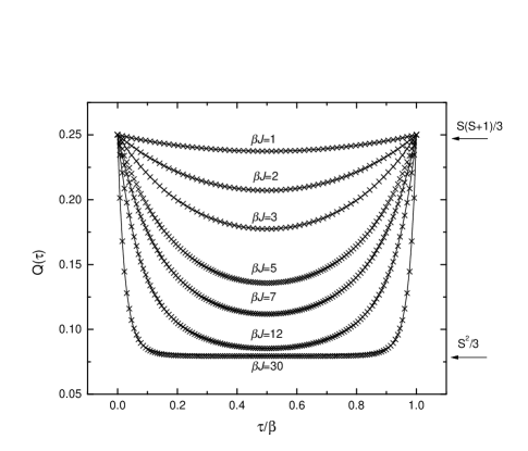
FIG. 1.: $Q(\tau)$ as function of $\tau/\beta$ for several values of $\beta J$. The crosses correspond to QMC data. The error bars are well below the size of the crosses. Solid lines are fits obtained with the function $Q_{par}(\tau)$ described in the text.

In Fig. 1 we show the correlation function obtained with this method which exhibits the following qualitative features. For $T>>J$, $Q(\tau)$ is nearly constant and close to $S(S+1)/3=1/4$, its classical limit. In contrast, for $T<<J$, $Q(\tau)$ rapidly decreases at both ends of the interval $[0,\beta]$ and then varies slowly remaining near the value $S^{2}/3$. The behavior in the intermediate temperature range is a smooth interpolation between the two extreme cases. We obtain $\chi_{loc}$ by numerically integrating $Q(\tau)$ and find that it crosses over between two limiting forms, $\chi_{loc}\approx S(S+1)/(3T)$ for $T>>J$ and $\chi_{loc}\approx S^{2}/(3T)$ for $T<<J$, implied by the asymptotic behavior of $Q(\tau)$ described above. The susceptibility thus obeys a Curie law at both ends of the temperature range with the low $T$ effective Curie constant reduced by a factor of 3 with respect to its classical value. Note that the low-temperature behavior of $\chi_{loc}(T)$ differs considerably from the prediction of the large-$M$ model[4] which is $\chi_{loc}(T)\sim\ln(1/T)$ for small $\kappa$. On the other hand, the full temperature dependence of $\chi_{loc}$ is remarkably close to that predicted by the variational approach[3]. This is easily understood at high and low temperatures where the variational ansatz of Bray and Moore[3], $Q(\tau)=const$, represents well the actual numerical solution (cf. Fig.1). However, the close agreement at intermediate temperatures is rather unexpected. The criterion for the appearance of spin glass order, $J\chi_{loc}=1$, is fulfilled at $T_{g}\approx 0.142J$ that compared to the classical value $T_{g}=0.25J$ shows the importance of quantum fluctuations in this system.

We now turn to the discussion of the frequency dependence of the local susceptibility. This involves extracting real-frequency information from results obtained on the imaginary axis, which is in general a rather difficult task. However, it will be seen below that in the present case the dissipative part of the local response $\chi^{\prime\prime}_{loc}(\omega)$ may be found analytically at low and high temperature. This allows us to construct an interpolating function that accurately describes our numerical data throughout the whole temperature range, enabling us to extract physical information from the imaginary-time Monte Carlo results.

The dynamics of the system for $T>>J$ is on general grounds expected to be controlled by a single relaxation rate ${\omega_{L}=\cal O}(J)$. This assumption implies

$$\frac{\chi^{\prime\prime}_{loc}(\omega)}{\pi\omega}=\chi_{loc}\frac{1}{\omega_{L}}F(\frac{\omega}{\omega_{L}}),$$ (8)

where the relaxation function $F$ is constrained to be normalized to one and have a finite second moment[6]. The simplest function fulfilling these conditions is a gaussian. With this ansatz, the response is completely determined by the sum-rule

$$\int_{-\infty}^{\infty}\frac{d\omega}{\pi}\omega\chi^{\prime\prime}_{loc}(\omega)=2J^{2}\int_{0}^{\beta}Q^{2}(\tau),$$ (9)

that is derived[7] using the generic $f$-sum rule for spin systems and (3). It then follows from (8) and (9) that

$$\frac{\chi^{\prime\prime}_{loc}(\omega)}{\pi\omega}=\frac{\beta S(S+1)}{3}\left[1-S(S+1){(\beta J)^{2}\over 18}\right]\frac{e^{-\frac{1}{2}(\frac{\omega}{\omega_{L}})^{2}}}{{\sqrt{2\pi\omega_{L}^{2}}}},$$ (10)

with $\omega^{2}_{L}=2J^{2}S(S+1)/3[1-S(S+1)(\beta J)^{2}/18]$ for $T>>J$. It can be shown[7] that Eq. 10 reproduces the first few orders of the high-temperature expansion of $Q(\tau)$. This expression is thus correct for $T>>J$.

With decreasing temperature, the assumption of a single relaxation rate breaks down. At $T<<J$ the existence of two different characteristic times suggested by the numerical data of Fig. 1 must be reflected in the emergence of well separated energy scales in the frequency dependent dynamic response. Indeed, this behavior follows from an approximate analytical solution of Eqs. 4 and 7 that can be shown to be exact in the $T\to 0$ limit. From Eq. 7 the problem can be thought of as that of a single spin in a fluctuating effective magnetic field $J\vec{\eta}(\tau)$. We will see below that at low $T$ this effective field is dominated by its $\omega_{n}=0$ component. Therefore, it is convenient to split the effective field into a constant part $\vec{h}_{0}=J\vec{\eta}(\omega_{n}=0)/\sqrt{\beta}$ and a small $\tau$-dependent part with $|\delta\vec{h}(\tau)|<<|\vec{h}_{0}|$. We thus write (4) as

$$Q(\tau)={1\over 3}\left[\langle Q_{L}(\tau,\vec{h}_{0})\rangle_{\vec{h}_{0}}+2\langle Q_{T}(\tau,\vec{h}_{0})\rangle_{\vec{h}_{0}}\right],$$ (11)

where $Q_{L}$ and $Q_{T}$ are, respectively, the longitudinal and transverse response functions in an applied field $\vec{h}_{0}$ having formally integrated out the fields $\delta{\vec{h}}(\tau)$. The angular brackets denote the average with respect to the isotropic distribution $P(|\vec{h}_{0}|)$. For a given $\vec{h}_{0}$, the imaginary part of the transverse response function $\chi^{\prime\prime}_{T}(\omega)$ has a peak at $\omega=|\vec{h}_{0}|$ whose width $\Gamma$ is proportional to the square of the amplitude of the fluctuating field at the resonance frequency. A simple estimate[8] shows that for $T<<J$, $P(|\vec{h}_{0}|)$ is maximum at $|\vec{h}_{0}|\equiv\omega_{T}\approx J^{2}S\chi_{loc}$, which is large at low temperature. Assuming for the moment that $|\delta\vec{h}(\tau)|<<|\vec{h}_{0}|$ (i.e., setting $\Gamma=0$) one can perform the average over $P(|\vec{h_{0}}|)$ and obtain an approximation for the dissipative part of $\langle Q_{T}(\tau,\vec{h}_{0})\rangle_{\vec{h}_{0}}$,

$$\frac{\chi^{\prime\prime}_{T}(\omega)}{\pi\omega}=\frac{S}{2}\left[\frac{\beta}{2\omega_{T}}\right]^{3/2}\frac{\omega\tanh(\beta\omega/2)}{\sqrt{2\pi}(1+\beta\omega_{T}/2)}$$ (12)

$$\times\left\{\exp\left[-\frac{\beta}{4\omega_{T}}(\omega-\omega_{T})^{2}\right]+\exp\left[-\frac{\beta}{4\omega_{T}}(\omega+\omega_{T})^{2}\right]\right\}.$$ (13)

Using this equation and the fluctuation-dissipation theorem we estimate $\Gamma/\omega_{T}={\cal O}(T/J)$, showing that the assumption leading to (13) is indeed correct. Therefore, the expression above is asymptotically exact for $T\to 0$.

The high-frequency scale $\omega_{T}\sim J^{2}/T$ where $\chi^{\prime\prime}_{T}(\omega)$ is sharply peaked, is associated to the initial rapid decrease in $Q(\tau)$ observed in our low-$T$ simulations. The remaining contribution to the dynamic response function $\chi^{\prime\prime}_{L}(\omega)$ comes from the relaxation of the longitudinal magnetization. As the amplitude of the fluctuating field $|\delta{\vec{h}(\tau)}|<<|\vec{h}_{0}|$ we expect this process to be slow. Its frequency $\omega_{L}$ may be found irrespectively of the detailed form of $\chi^{\prime\prime}_{L}(\omega)$ using Eqs. 9, 11 and 13 which yield $\omega_{L}\propto T^{2}$ [7]. This small energy scale is associated to the slowly varying part of $Q(\tau)$ observed at low temperature. Using again the ansatz (8) for $\chi^{\prime\prime}_{L}(\omega)$, the sum-rule (9) leads to an expression similar to (10), except that the prefactor of the exponential is now simply $\beta S^{2}/3$. Notice that the dynamics of magnetic fluctuations that emerges from the above arguments bears no resemblance to that of the spin-fluid state of the large-$M$ model.

Comparison between the low- and high-temperature results implies that when $T$ decreases, a fraction of the spectral weight of the quasi-elastic peak at small-$\omega$ is transferred to the high energy excitations described by Eq. 13. This redistribution of intensity, closely related to the reduction of the effective Curie constant discussed above, is a distinctive quantum effect: the strength of the inelastic feature relative to that of the quasi-elastic peak is ${\cal O}(1/S)$ and vanishes in the large-$S$ limit. The analytical results just discussed suggest a parametrization of the spin-spin correlation function $Q(\tau)$ that contains the exact asymptotic forms at both high and low $T$ and smoothly interpolates between them. The proposed interpolation function is defined as $Q_{par}(\tau)=S(S+1)/3[p\Phi_{L}(\tau)+(1-p)\Phi_{T}(\tau)]$ where,

$$\Phi_{L}(\tau)=e^{-\frac{1}{2}\left(\frac{\beta\omega_{L}}{2}\right)^{2}\left[1-\left(1-\frac{2\tau}{\beta}\right)^{2}\right]}$$ (14)

$$\Phi_{T}(\tau)=\frac{1+\beta\omega_{T}/2\left(1-2\tau/\beta\right)^{2}}{1+\beta\omega_{T}/2}e^{-\frac{\beta\omega_{T}}{4}\left[1-\left(1-\frac{2\tau}{\beta}\right)^{2}\right]},$$ (15)

where $\Phi_{L}$ and $\Phi_{T}$ are the imaginary-time equivalents of Eqs. 10 and 13 normalized such that $\Phi_{L,T}(0)=1$, and $\omega_{L}$ and $\omega_{T}$ are now parameters corresponding to the width of the central peak and the characteristic scale of the high-energy excitations, respectively. The third parameter, $p$, controls the transfer of spectral weight between the two components of the magnetic response. At high $T$ there is a single energy scale and only quasi-elastic intensity is present as $p\to 1$, while at low $T$ inelastic intensity appears and $p\to S/(S+1)$ its lower bound.

Using this expression we obtain highly accurate fits of our numerical results as demonstrated in Fig. 1. While $Q_{par}(\tau)$ contains the correct high and low $T$ limits by construction, it is remarkable that the quality of the agreement remains excellent through all the temperature range. This gives us confidence that the essential physics is indeed captured by our parametrization of $Q(\tau)$. It is now interesting to go back to real frequency and plot $\chi^{\prime\prime}_{loc}(\omega)/\omega$ which is an experimentally accessible quantity. The results shown in Fig. 2 illustrate the gradual emergence of the high-frequency features in the dynamic response.

FIG. 2.: The relaxation function $F(\omega)=\chi^{\prime\prime}(\omega)/(\pi\chi_{loc}\omega)$ for $\beta J$ = 3 (long dashed), 7 (dashed) and 14 (solid). Inset: $T-$dependence of the parameters $p$ (circles) and $\omega_{L}$ (squares) that have the limiting behavior predicted by the theory.

Our results are strictly valid above $T_{g}$, since below this temperature the paramagnetic state is unstable [9]. Nevertheless, the study of the solution in the whole $T-$range is justified as it should be kept in mind that the precise value of $T_{g}$ depends on the details of the model Hamiltonian. For instance, lowering the dimensionality will enhance the role of fluctuations which in turn are expected to reduce the value of the transition temperature. Therefore, the qualitative properties of our paramagnetic solution may be relevant for real quantum spin glasses in their disordered phase. In this context two predictions that emerge from our work may provide useful insight for the analysis of experiments on quantum frustrated systems [10] provided that $T_{g}$ is small enough. i) Measurements of the magnetic susceptibility as the transition is approached from above may indicate an anomalously low value of the effective Curie constant. ii) For $T\geq T_{g}$ a fraction of the spectral weight may be spread over a wide energy range and be difficult to distinguish from background noise. This fact, combined with the presence of a very strong and narrow central peak, may result in an apparent loss of spectral weight in neutron scattering experiments.

Many interesting questions remain to be addressed, for instance, the effect of coupling the spin-system to an electronic band. For a bandwidth larger than $J$ one may expect that $T_{g}\to 0$ leading to the interesting physics of systems near quantum critical points [11].

REFERENCES

- [1] D. Sherrington and S. Kirkpatrick, Phys. Rev. Lett. 35, 1792 (1975).
- [2] K. H. Fischer and J. A. Hertz, “Spin Glasses”, Cambridge University Press, Cambridge (1991).
- [3] A. J. Bray and M. A. Moore, J. Phys. C 13, L655 (1980).
- [4] S. Sachdev and J. Ye, Phys. Rev. Lett. 70, 3339 (1993).
- [5] For recent work on quantum fluctuations in related models see, for instance: T. K. Kopeć and K. D. Usadel, Rev. Lett. 78, 1988 (1997). S. Sachdev and A. P. Young, Phys. Rev. Lett., 78, 2220 (1997). H. Rieger and A. P. Young, (unpublished) cond-mat/9607005.
- [6] D. Forster, “Hydrodynamic Fluctuations, Broken Symmetry, and Correlation Functions”, Addison-Wesley, NY (1990).
- [7] D. R. Grempel and M. J. Rozenberg, (unpublished).
- [8] This estimate is be obtained by evaluating the probability associated with Eq.7 for a -independent field.
- [9] The same remark applies to the spin fluid phase of the large Hamiltonian which cannot be the true ground state. The behavior implies that the criterion for a spin glass transition is satisfied at a finite .
- [10] S. M. Hayden, et al., Phys. Rev. Lett. 76, 1344 (1996). F. C. Chou, et al., Phys. Rev. Lett. 75, 2204 (1995).
- [11] S. Sachdev and N. Read, J. Phys. Condens. Matter 8, 9723 (1996).