Magnetic sublayers effect on the exchange coupling oscillations vs. cap-layer thickness

Abstract

We have found that some periods of interlayer exchange coupling (IEC) oscillations as a function of cap-layer (CL) thickness may be suppressed if the in-plane extremal spanning vectors of the cap- and ferromagnet-materials Fermi surfaces do not coincide. The suppression of the IEC oscillations vs. the CL thickness holds also if the magnetic slab thickness tends to infinity. On the one hand, we have shown by means of very simple arguments that apart from the well-known selection rules concerning the spacer- and cap-layers, another one related with the magnetic sublayers has to be fulfilled in order that the interlayer coupling oscillations $vs.$ CL thickness could survive. On the other hand, the distribution of induced magnetic moments across the non-magnetic cap- and spacer-sublayers have been computed and shown to reveal the underlying periodicity of the materials they are made of (i.e. related to their bulk Fermi surfaces) independently of whether or not the selection rules are fulfilled. This means that the IEC oscillations are of global nature and depend on all the sublayers the system consists of.

(Received ……………… 1997)

I Introduction

Magnetic multilayers have been intensively studied for over a decade now [1, 2, 3]. The reasons for it, apart from challenging cognitive aspects, are (already partially realized) practical applications of superlattices as magneto-resistive sensors, angular velocity meters, recording heads and magnetic memory elements. The phenomenon most of these applications is based on is the well known giant magneto-resistance (GMR) coming from a strong electron-spin dependence of resistivity in magnetic systems. To optimize devices of that sort, it is necessary to test the effect of all of the ingredients of the system in question (including kind of materials they are made from and thicknesses of particular sublayers), either directly on GMR or indirectly on the interlayer exchange coupling (IEC). Obviously, the effect of a spacer on IEC was established first [3, 4], the next in turn was that due to magnetic sublayers [5, 6, 7, 8, 9, 10] and finally the cap-layer (CL) effect has been studied quite recently [11, 12, 13, 14, 15].

Before we present our original results let us briefly recall what are the most important facts concerning the CL’s : i) the IEC oscillates as a function of CL thickness with a period determined by extremal $\vec{k}$ spanning vectors of the CL Fermi surface, ii) a bias of the oscillations (their asymptotic value) depends on spacer thickness [11, 14, 15], iii) the IEC oscillations are strongly suppressed if stationary in-plane spanning vectors of the CL Fermi surface do not coincide with their counterparts of the spacer Fermi surface[14, 15], iv) the direct- and inverse-photoemission[16, 17] on various combinations of overlayers deposited on different films shows a periodic distribution of the so-called quantum well states (QWS) with periods determined by extremal spanning vectors of the overlayer Fermi surface. We shall refer to the latter only indirectly, by exploiting the fact that the QWS lead to some spin-polarization of non-magnetic cap-layers.

The aim of the present paper is to emphasize the relevance of magnetic sublayers to IEC oscillations as a function of cap-layer (CL) thickness. Besides, we shall comment on induced magnetic moments in the non-magnetic sublayers, which may be viewed as a manifestation of the quantum well states [16, 17, 18, 19].

II Method

Our earlier papers [6, 20, 21] based on the single-band tight-binding model have proved that the model we use gives a reasonable qualitative description of basic physical mechanisms responsible for oscillatory phenomena in magnetic trilayers.

Our Hamiltonian, described in detail in Ref. [21], consists of the nearest-neighbor hopping and spin-dependent on-site potential terms. The systems under consideration now are trilayers capped with an overlayer, of the type $n_{ovr}O/n_{f}F/n_{s}S/n_{f}F$, where $n_{ovr}$, $n_{f}$ and $n_{s}$ stand for the numbers of cap- (O), ferromagnet- (F) and spacer- (S) monolayers in the perpendicular $z$-direction. Hereafter the subscripts and superscripts $ovr$ and $s$ will always refer to the cap- and spacer-layers, whereas the spin-dependent parameters referring to ferromagnetic sublayers will be indexed by $\sigma=\uparrow$ or $\downarrow$. For simplicity, we restrict ourselves to a simple cubic structure and regard the lattice constant and the hopping integral as the length- and energy-units, respectively.

The interlayer exchange coupling has been calculated from the difference in thermodynamic potentials exactly as in Ref. [21], moreover the magnetic moments (including the induced ones), $m$, have been expressed in terms of the eigen-functions $u$ of the Hamiltonian as $m_{i}=n_{i\uparrow}-n_{i\downarrow}$, with $n_{i\sigma}=\sum\limits_{E}|u_{i,\sigma}(E)|^{2}$, where the summation runs over occupied states.

III Asymptotic limits

In this section we present some analytic formulae which will be useful for interpretation of rigorous numerical resluts of the next section. As has been shown in Ref. [22], the IEC can be Fourier-transformed with respect to $n_{s}$ and $n_{\sigma}$. That procedure can be quite straightforwardly generalized to include CL thickness as well. The resulting asymptotic (within the stationary phase approximation) expression consists of the terms of the form $A_{pqrn}(\vec{k}_{\|},E_{F})exp\left(2i(pk^{s}_{z}n_{s}+(qk^{\uparrow}_{z}+rk^{\downarrow}_{z})n_{f}+nk^{ovr}_{z}n_{ovr})\right)$ summed over all the in-plane wave vectors for which the exponential is stationary. The $A$ coefficients are defined analogously as in Ref. [22]. Their exact numerical values are not important for qualitative considerations, one notes only that all the amplitudes of oscillations vanish asymptotically with the given sublayer thickness going to infinity[22]. There exist, however, some additional restrictions imposed by the asymptotic behavior of the IEC. In particular, a direct generalization of the results of Ref. [22] to the present case, with the cap-layer, gives: $A_{0qrn}=0$ (no coupling for $n_{s}\rightarrow\infty$). Another limit to be taken is $n_{f}\rightarrow\infty$, when, in view of the above mentioned asymptotic behavior, all the terms tend to zero except for $A_{p000}$ and $A_{p00n}$. Since the oscillations vs. spacer thickness survive in this limit in contrast to the ones vs. CL thickness which decay (see below), we conclude that $A_{p000}\neq 0$ and $A_{p00n}=0$.

Finally, taking into account the above mentioned restrictions and keeping for simplicity only the lowest order harmonics, we arrive at the following formula :

$$J = \sum_{\alpha}A_{1000}e^{2ik^{s}_{z}n_{s}}+\sum_{\alpha_{1}}A_{1100}e^{2i(k^{s}_{z}n_{s}+k^{\uparrow}n_{f})}+\sum_{\alpha_{2}}A_{1010}e^{2i(k^{s}_{z}n_{s}+k_{z}^{\downarrow}n_{f})}$$ (1)

$$+\sum_{\alpha_{3}}A_{1101}e^{2i(k^{s}_{z}{n}_{s}+k^{\uparrow}_{z}n_{f}+k_{z}^{ovr}n_{ovr})}+\sum_{\alpha_{4}}A_{1011}e^{2i(k_{z}^{s}n_{s}+k_{z}^{\downarrow}n_{f}+k_{z}^{ovr}n_{ovr})}+\ldots,$$ (2)

where the $\alpha$-s are the sets of in-plane wave vectors for which the relevant exponentials are stationary. For the case of the CL thickness dependence this allows us to formulate the following new selection rule, which in its general form (for $n_{s}$ and $n_{f}$ large and fixed and $n_{ovr}$ large and varying) reads :

$$\nabla k^{ovr}_{z}=0,\;\;p\nabla k^{s}_{z}n_{s}+(q\nabla k^{\uparrow}_{z}+r\nabla k^{\downarrow}_{z})n_{f}=0,$$ (3)

with nonvanishing $p$ and either $q$ or $r$ ($\nabla$ is the two-dimensional gradient in the $k_{x}$,$k_{y}$ space). This means that out of all the stationary vectors of the cap material FS only those which simultaneously satisfy the above mentioned conditions for the in-plane gradients give rise to the oscillations with CL thickness. Eq. (3) is the main result of the present paper. This condition becomes even simpler in the particular case of the single–band simple cubic model considered hereafter, when the second part of Eq. (3) separates and all the individual in-plane gradients must vanish (c.f. Ref. [22]).

The origin of the new selection rule becomes clear if we qualitatively interpret Eq. (1) in terms of the quantum interference model[23]. The first term corresponds to the states reflected once at each of the spacer-ferromagnet interfaces, the second and third ones to the states penetrating one of the magnetic layers and reflected back at the cap-ferromagnet interface while the last two terms describe states reaching the outer boundary of the cap-layer (“vacuum”). It is quite clear therefore that the $n_{f}$-dependent phase factor must be also taken into account while performing the stationary phase approximation.

It is evident from formula (1) that the bias of oscillations with CL thickness depends not only on the spacer- and magnetic- layer thicknesses but on the on-site $V^{ovr}$ potential as well. The latter observation results from the fact that the $A$ coefficients in the second and third terms of Eq. (1) depend on the value of the reflection coefficient at the cap-ferromagnet interface which in turn depends on the cap material electronic structure.

The stationary spanning vectors, for a sublayer characterized by the potential $V$, can be determined in a very simple way, by minimizing with respect to $\vec{k}_{\|}$ the following Fermi surface equation for the s.c. lattice :

$$k_{z}(\vec{k}_{\|},E_{F})=\arccos[(V-E_{F})/2-\cos k_{x}-\cos k_{y}]\,.$$ (4)

Hence the in-plane extremal spanning vectors are: $\vec{k}_{\|}=(0,0)$ for $-6<E_{F}-V<-2$; $(\pm\pi,0)$ $(0,\pm\pi)$ for $-2<E_{F}-V<2$; $(\pm\pi,\pm\pi)$ for $2<E_{F}-V<6$ and

$$k_{z}=\arccos[(V-E_{f})/2-\alpha]\,,$$ (5)

with $\alpha=$ 2, 0 and -2, for the corresponding $\vec{k}_{\|}$, respectively. Thus, the period of oscillations $vs.$ sublayer (with the potential $V$) thickness, is just $\Lambda=\pi/{k_{z}}$ (or $\pi/{(\pi-k_{z})}$).

IV Numerical results

We shall now present our exact numerical results (see Ref. [21] for details of the method) and show how they can be interpreted in terms of the analytical formulae from the preceding section. Fig. 1. confirms the well-known fact that the IEC oscillations vs. CL thickness have got a period determined by kind of material the cap is made of and get suppressed if there is a mismatch in corresponding in-plane spanning vectors of the CL and the spacer. The suppression takes place in the cases $c$ and $d$ where ${\vec{k}_{\|}}^{s}={\vec{k}_{\|}}^{\sigma}=({\pm\pi,\pm\pi})$, opposite to ${\vec{k}_{\|}}^{over}=({0,\pm\pi})$,$(\pm\pi,0)$. The dependence of the bias values on $V^{ovr}$ is also clearly visible. The new effect is presented in Fig. 2, which shows that the suppression may be due to the misfit in the ${\vec{k}_{\|}}$’s corresponding to the overlayer and magnetic sublayers, respectively (curves $c$ and $d$), whereas in case of the curves $a$ and $b$ the periodicity is quite pronounced owing to the matching of the above mentioned spanning vectors. It can be also readily seen from Fig. 2 that the phases of oscillations as well as the bias-values depend on the potentials of the ferromagnetic layers (exchange splitting). It is noteworthy that Figs. 1 and 2 show that the selection rule works quite well, even when the relevant layer thicknesses are rather small: $n_{s}=5$ and $n_{f}=10$, respectively. This confirms our previous observation[21] that relatively small systems in the z-direction may reveal the asymptotic behavior. A detailed inspection of curves c and d suggests that the selection rule is slightly more rigorously enforced in Fig. 2 (due to $n_{f}=10$) than in Fig. 1 (due to $n_{s}=5$), but the effect is tiny indeed and hardly visible. Incidentally, all the periods of oscillations obtained by the numerical computations and visualized in Figs. 1–4 can be pretty well reproduced in terms of the asymptotic Eqs. (4) and (5): e.g. for $E_{F}=2.1$ and $V=-0.6,\,-0.3,\,0.0,\,0.3$ and $0.6$, we get $\Lambda=3.6,\,4.9,\,9.9,\,6.9$ and $4.3$ ML respectively.

Another rather obvious but noteworthy effect consists in vanishing of the IEC oscillations vs. CL thickness when magnetic sublayer thickness gets bigger and bigger. This is shown in Fig. 3, and has not been discussed either, to our knowledge so far, although such a trend could be predicted on the basis of analytical formulae of Ref. [14]. In fact this finding means that in order to avoid undesirable effects of cap-layers (which may be of different thickness in an experiment) on the IEC oscillations one should work with thick magnetic sublayers. It is also noteworthy that the oscillation bias value depends on the magnetic layer thickness, as could be predicted from Eq. 1.

Finally, in connection with the quantum well states concept[16, 17, 18, 19], we have studied the distribution of induced magnetic moments in the CL (and in the spacer). A typical result is presented in Fig. 4. The induced magnetic moments are measured in dimensionless units ($\mu_{B}=1$) and are of the order of 0.1% with respect to the magnetic layer magnetization. As expected, the period of the induced-moment distribution within the CL is exactly that anticipated for the bulk CL material FS. The effect of the other sublayers is minor, except that the magnitude of the induced moments is also magnetic-slab dependent. This might seem, at a first glance, to be in conflict with the IEC behavior which shows no oscillations for parameters of Fig. 4 (cf. Fig. 1c). Yet the spin polarization in non-magnetic layers is related to just one system with the fixed sublayer thicknesses and the given alignment of magnetic sublayers, whereas the IEC results from the total energy (thermodynamic potential) balance between the two possible ferromagnetic layer alignments and has to do with the series of samples with changing CL thicknesses. This observation implies that the induced-magnetic moments in the non-magnetic cap-layer (as well as the QWS) give in general the whole set of periods, out of which only those survive, as far as the IEC is concerned, which fulfill the selection rules referring to the entire system. In other words the IEC oscillations are the global characteristic of the whole system, whereas the induced spin polarization in the cap-layer is strictly of local nature.

The selection rules completed hereby by the extra condition related with the extremal spanning vectors of the magnetic sublayers, are quite general and apply to real systems, too. In particular they allow to explain why in case of the Cu/Co/Cu/Co multilayer the short period of oscillations with Cu cap-layer thickness is absent[11] in spite of theoretical predictions [14] and the photoemission results concerning QWS [16, 17, 19]. In fact the explanation is simple and quite analogous to that of Ref. [22] about IEC oscillations as a function of ferromagnetic layer thickness. Out of two in-plane extremal spanning vectors of the Cu Fermi surface only the “belly” one (at $\vec{k}_{\|}=0$ ) coincides with the extrema of the majority and minority sheets of the Co Fermi surface, giving rise to the long period of oscillations. The “neck” spanning vector has no counterpart in the Co FS and this is why there are no short period oscillations.

In conclusion, we have shown that in order for the interlayer exchange coupling oscillations vs. cap-layer thickness to exist, it is necessary, that both the cap-layer- and magnetic-layer- Fermi surfaces share the same extremal in-plane spanning vectors. If this new “selection rule” is not fulfilled the period anticipated from the bulk cap-layer material will not occur in the exchange coupling, although it will still be present in the induced moment distribution across the cap layer. Another finding of this paper is that the IEC oscillations vs. CL - thickness vanish if magnetic sublayers thickness tends to infinity.

This work has been carried out under the KBN grants No. 2P03B 165 10 (MZ) and 2-P03B-099-11 (SK). We thank the Poznań Supercomputing and Networking Center for the computing time.

List of Figures

lof

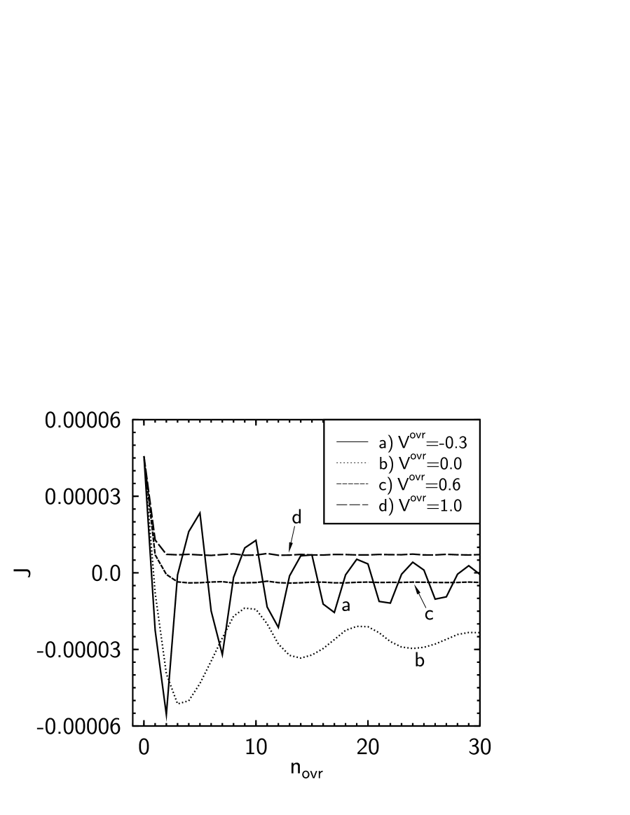
FIG. 1.: The exchange coupling vs. cap layer thickness for $n_{s}=5$, $n_{f}=3$, $E_{F}=2.1$, $V^{s}=V^{\downarrow}=0$ and $V^{\uparrow}=-2.0$. Stationary in-plane spanning vectors of the spacer and both the ferromagnetic FS’s are $k_{\|}=(\pm\pi,\pm\pi)$. For the curves $a$ and $b$ the stationary in-plane vector of the cap FS is the same in contrast with the $c$ and $d$ cases, for which $k_{\|}=(0,\pm\pi),(\pm\pi,0)$ what results in suppressing the oscillations.

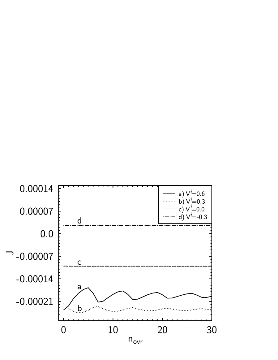
FIG. 2.: IEC vs. CL thickness for $n_{s}=5$, $n_{f}=10$, $E_{F}=2.1$, $V^{s}=V^{ovr}=0.3$ and $V^{\uparrow}=-2.0$. Stationary in-plane spanning vectors for the spacer and the cap-layer are $k_{\|}=(0,\pm\pi),\,(\pm\pi,0)$. For the first two curves ($a$ and $b$) the minority spin FS stationary points coincide with those of the spacer and the overlayer. In case of the curves $c$ and $d$ both the majority and minority spin Fermi surfaces have the $k_{\|}=(\pm\pi,\pm\pi)$ spanning vector and consequently the IEC oscillations are suppressed.

FIG. 3.: The effect of magnetic sublayer thickness on the IEC oscillations as a function of cap-layer thickness (parameters as in Fig. 1 except for $V^{ovr}=-0.6$).

FIG. 4.: Induced magnetic moments (with $\mu_{B}=1$) for $n_{s}=n_{ovr}=40$ and $n_{f}=10$ for parallel (full line) and antiparallel (dashed line) configurations. The other parameters as in Fig. 1c. Thick vertical lines mark the interfaces.

REFERENCES

- [1] P. Grünberg, R. Schreiber, Y. Pang, M.B. Brodsky, and H. Sower, Phys. Rev. Lett. 57, 2442 (1986)
- [2] S.S.P. Parkin, in Ultrathin Magnetic Structures, edited by B. Heinrich, and J.A.C. Bland (Springer-Verlag, Berlin, 1994,Vol. 2, p.148); A. Fert and P. Bruno, (ibid, p.82)
- [3] P. Bruno and C. Chappert, Phys. Rev .Lett. 67, 1602 (1991)
- [4] D.M. Edwards, J. Mathon, R.B. Muniz, and M.S. Phan, J. Phys.:Cond. Matt. 3, 4941 (1991)
- [5] J. Barnaś, J.Magn.Magn.Mater. 111, L215 (1992)
- [6] S. Krompiewski, J.Magn.Magn.Mater. 140-144, 515 (1995)
- [7] S. Krompiewski, F. Süss, and U. Krey, Europhys. Lett. 26, 303 (1994)
- [8] P. Bruno, Europhys. Lett. 23, 615 (1993)
- [9] P.J.H. Bloemen, M.T. Johnson, M.T.H. van de Vorst, R. Coehoorn, J.J. de Vries, R. Jungblut, J. aan de Stegge, A. Reinders, and W.J.M. de Jonge, Phys. Rev. Lett. 72, 764 (1994)
- [10] S.N. Okuno and K. Inomata, Phys. Rev. B 51, 6139 (1994)
- [11] J.J. de Vries, A.A.P. Schudelaro, R. Jungblut, P.J.H. Bloemen, A. Reinders, J. Kohlhepp, R. Coehoorn and, W.J.M. de Jonge, Phys. Rev. Lett. 75, 4306 (1995)
- [12] S.N. Okuno and K. Inomata, J. Phys. Jap. 64, 3631 (1995)
- [13] J.Barnaś, Phys. Rev. B 54, 12332 (1996)
- [14] P. Bruno, J. Magn. Magn. Mater. 164, 27 (1996)
- [15] J. Kudrnovský, V. Drchal, P.Bruno, I. Turek, and P. Weinberg, Phys. Rev. B 56, 8919 (1997)
- [16] J.E. Ortega, F.J. Himpsel, G.J. Mankey, and R.F. Willis, Phys. Rev. B 47, 1540 (1993)
- [17] J.E. Ortega and F.J. Himpsel, Phys. Rev. Lett. 69, 844 (1992)
- [18] Q.Y. Jin, Y.B. Xu, H.R. Zhai, C. Hu, M. Lu, Q.S. Bie, Y. Zhai, G.L. Dunifer, R. Naik, and M.Ahmad, Phys. Rev. Lett. 72, 768 (1994)
- [19] P. Segovia, E.G. Michel and J.E. Ortega, Phys. Rev. Lett. 77, 3455 (1996)
- [20] S. Krompiewski and U. Krey, Phys. Rev. B 54, 11961 (1996).
- [21] S. Krompiewski, M. Zwierzycki, and U. Krey, J. Phys.:Cond.Matt. 9, 7135 (1997)
- [22] J. d’Albuquerque e Castro, J. Mathon, M. Villeret, and D.M. Edwards, Phys. Rev. B 51, 12876 (1995)
- [23] P. Bruno, Phys. Rev. B 52, 411 (1995)