Quantum Hall Fluids on the Haldane Sphere:
A Diffusion Monte Carlo Study

Abstract

A generalized diffusion Monte Carlo method for solving the many-body Schrödinger equation on curved manifolds is introduced and used to perform a ‘fixed-phase’ simulation of the fractional quantum Hall effect on the Haldane sphere. This new method is used to study the effect of Landau level mixing on the $\nu=1/3$ energy gap and the relative stability of spin-polarized and spin-reversed quasielectron excitations.

Much of the modern understanding of the fractional quantum Hall effect (FQHE) is based on the observation that in two dimensions the quantum statistics of identical particles can be changed by performing a singular gauge transformation [1]. Such a transformation can be used, for example, to map the equations describing an ideal two dimensional electron gas in a transverse magnetic field at Landau level filling factor $\nu=1/q$, where $q$ is an odd integer, into those describing a system of ‘composite bosons’ moving in zero effective magnetic field, interacting via both Coulomb and ‘Chern-Simons’ interactions. This transformation, from fermions to bosons, is the basis of the successful Chern-Simons-Landau-Ginzburg phenomenology of the FQHE [2]. Its existence also suggests the possibility of numerically simulating the FQHE at $\nu=1/q$ using the composite boson description.

Recently, Ortiz, Ceperley, and Martin (OCM) [3] introduced the ‘fixed-phase’ diffusion Monte Carlo (DMC) method for simulating non-time-reversal symmetric systems with complex-valued eigenfunctions. OCM applied this method to the FQHE ground state at $\nu=1/q$, using the torus geometry, and fixing the phase of the wave function with Laughlin’s trial wave function. The resulting effective bosonic problem corresponded precisely to the composite boson description, with the additional approximation that those terms in the transformed Hamiltonian leading to fluctuations of the phase of the wave function were ignored. This effective bosonic problem was then solved by standard DMC techniques [4], and the results used to study the effect of Landau level mixing (LLM) on the FQHE ground state. However, OCM did not consider either excited states or geometries other than the torus.

In this Letter we present the results of a ‘fixed-phase’ DMC study of the FQHE at $\nu=1/3$ using the spherical geometry introduced by Haldane [5]. In order to go from the torus to the sphere we introduce a generalized DMC method for solving the many-body Schrödinger equation on curved manifolds. One motivation for this work is that the ‘Haldane sphere’ is arguably the most convenient geometry for numerical study of the FQHE, and we believe that our generalization of the fixed-phase DMC method to this geometry will be useful for many future calculations. As an example of the application of this new method we have calculated the effect of LLM on the FQHE transport gap, i.e., the energy gap for creating a fractionally charged quasielectron – quasihole pair with infinite separation. Results have been obtained for both a spin-polarized and spin-reversed quasielectron. Previous calculations of the crossover magnetic field below which the transport gap is set by the spin-reversed excitation have ignored LLM [6, 7]. The present work includes these effects for the first time.

An ideal two dimensional electron gas, with effective mass $m^{*}$, carrier density $n$ and dielectric constant $\epsilon$, placed in a transverse magnetic field $B$ is characterized by three length scales — the effective Bohr radius $a_{B}=\epsilon\hbar^{2}/m^{*}e^{2}$, the magnetic length $l_{0}=\sqrt{\hbar c/eB}$, and the mean interparticle spacing $d=1/\sqrt{\pi n}$. These length scales can be combined to form two independent dimensionless ratios, the filling factor $\nu=2l_{0}^{2}/d^{2}$, and the electron gas parameter $r_{s}=d/a_{B}$. The degree of LLM is characterized by the ratio of the typical Coulomb energy to the cyclotron energy $(e^{2}/\epsilon d)/\hbar\omega_{c}=r_{s}\nu/2$ where $\omega_{c}=eB/m^{*}c$. Thus, for fixed $\nu$, $r_{s}$ provides a useful measure of the importance of LLM. Because $r_{s}\propto m^{*}/\sqrt{B}$ LLM can be increased either by decreasing $B$ or increasing $m^{*}$. For example, in two dimensional GaAs/AlGaAs systems with typical carrier densities, for $n$-type systems $m^{*}\simeq 0.07$ and $r_{s}\sim 2$ while for $p$-type systems $m^{*}\simeq 0.38$ and $r_{s}\sim 10$.

In the spherical geometry electrons are confined to the surface of a sphere of radius $R$ with a magnetic monopole at its center. Let $N$ denote the number of electrons and $2S$ denote the number of flux quanta piercing the surface of the sphere. The field strength is then $B=S\hbar c/eR^{2}$ and, for $\nu=1/q$, $2S=q(N-1)$. If electron positions are given in stereographic coordinates, ${\bf r}=(x,y)=(\cos\phi,\sin\phi)\tan\theta/2$ where $\theta$ and $\phi$ are the usual spherical angles, then the Hamiltonian is, in appropriately scaled atomic units ($\hbar=m^{*}=e^{2}=1$),

$$H=\frac{1}{2}\sum_{i}D({\bf r}_{i})(-i{\bf\nabla}_{i}+{\bf A}({\bf r}_{i}))^{2}+\frac{1}{\epsilon}\sum_{i<j}\frac{1}{\sqrt{r_{ij}^{2}+\beta^{2}}}\ ,$$ (1)

where $D({\bf r}_{i})=(1+r_{i}^{2})^{2}/4R^{2}$, $r_{ij}$ is the chord distance on the sphere, and $\beta$ is a parameter which models the finite thickness of the 2DEG [8]. We work in the Wu-Yang [9] gauge for which ${\bf A}({\bf r}_{i})=2R^{2}B(-y_{i},x_{i})/(1+r_{i}^{2})$.

In what follows we have used three trial wave functions to implement the fixed-phase approximation ($z=x+iy$ is the complex stereographic coordinate):

(i) Ground state.— In the Wu-Yang gauge the spherical analog of the Laughlin wave function for $\nu=1/q$ is [5]

$$\psi_{\rm GS}=\prod_{k}(1+|z_{k}|^{2})^{-S}\prod_{i<j}(z_{i}-z_{j})^{q}\ .$$ (2)

(ii) Spin-polarized excited state.— For this state we have used the following wave function, constructed using Jain’s composite fermion approach [10], describing an excitation with a charge $e/q$ quasielectron at the top of the sphere and a charge $-e/q$ quasihole at the bottom of the sphere,

$$\psi_{\rm SP}=\prod_{k}(1+|z_{k}|^{2})^{-S}\prod_{i<j}(z_{i}-z_{j})^{q-1}\left|\begin{array}[]{ccccc}1&z_{1}&...&z_{1}^{N-2}&\sum_{i\neq 1}\frac{1}{z_{1}-z_{i}}\\ \vdots&\vdots&&\vdots&\vdots\\ 1&z_{N}&...&z_{N}^{N-2}&\sum_{i\neq N}\frac{1}{z_{N}-z_{i}}\\ \end{array}\right|\ .$$ (6)

(iii) Spin-reversed excited state.— This state is similar to $\psi_{\rm SP}$ except the quasielectron has a reversed spin. If $z_{1}$ denotes the coordinate of the down spin electron then this wave function is [7]

$$\psi_{\rm SR}=\prod_{k}(1+|z_{k}|^{2})^{-S}\prod_{l\neq 1}(z_{l}-z_{1})^{-1}\prod_{i<j}(z_{i}-z_{j})^{q}\ .$$ (7)

The fixed-phase approximation is carried out as follows. First, the relevant trial function is written as $\psi_{\rm T}({\cal R})=|\psi_{\rm T}({\cal R})|\ \exp[i\phi_{\rm T}({\cal R})]$, where ${\cal R}=({\bf r}_{1},{\bf r}_{2},\cdots,{\bf r}_{N})$. The overall phase $\phi_{\rm T}({\cal R})$ is then used to perform a singular gauge transformation, $\hat{H}=\exp[-i\phi_{\rm T}({\cal R})]\ H\ \exp[i\phi_{\rm T}({\cal R})]=H_{\rm R}+iH_{\rm I}$, where

$$H_{\rm R} = -\frac{1}{2}\sum_{i}D({\bf r}_{i})(\nabla^{2}_{i}-\tilde{\bf A}^{2}({\bf r}_{i}))+\frac{1}{\epsilon}\sum_{i<j}\frac{1}{\sqrt{r_{ij}+\beta^{2}}},$$ (8)

$$H_{\rm I} = -\frac{1}{2}\sum_{i}D({\bf r}_{i})\left({\bf\nabla}_{i}\cdot\tilde{\bf A}({\bf r}_{i})+\tilde{\bf A}({\bf r}_{i})\cdot{\bf\nabla}_{i}\right)\ ,$$ (9)

and $\tilde{\bf A}({\bf r}_{i})={\bf A}({\bf r}_{i})+{\bf\nabla}_{i}\phi_{\rm T}({\cal R})$. As shown by OCM, the bosonic ground state of $H_{\rm R}$ is the lowest energy state with the same phase as the trial function [3]. The DMC method can then be applied to the imaginary time Schrödinger equation $H_{\rm R}\psi({\cal R},t)=-\frac{\partial}{\partial t}\psi({\cal R},t)$, the solution of which, in the limit $t\rightarrow\infty$, converges to the ground state of $H_{\rm R}$.

The dependence of $D({\bf r})$ on position in (1) is a consequence of the finite curvature of the surface of the sphere, for which the metric tensor, in stereographic coordinates, is $g_{\alpha\beta}({\bf r})=D({\bf r})^{-1}\delta_{\alpha\beta}$. Below we introduce our generalized DMC method for simulating the many-body Schrödinger equation on such a curved manifold. Note that in two dimensions it is always possible to choose coordinates for which $g_{\alpha\beta}=f({\bf r})\delta_{\alpha\beta}$, i.e., to work in the so-called ‘conformal gauge’, and so the generalized DMC method introduced below can, in principle, be applied to any curved two-dimensional manifold, not just the sphere.

The central modification of the DMC method required to treat the present problem is to replace the usual importance-sampled distribution function $P({\cal R},t)=\psi({\cal R},t)|\psi_{\rm T}({\cal R})|$ [4] with

$$\widetilde{P}({\cal R},t)=\psi({\cal R},t)|\psi_{T}({\cal R})|\prod_{i=1}^{N}\frac{1}{D({\bf r}_{i})}\ .$$ (10)

This has two important consequences. First, because the differential area element on the sphere is $dA=d^{2}r/D({\bf r})$ the expectation value of the ground state energy is simply

$$\langle H\rangle=\frac{\int\widetilde{P}({\cal R},t\rightarrow\infty)E_{L}({\cal R})d{\cal R}}{\int\widetilde{P}({\cal R},t\rightarrow\infty)d{\cal R}}\ .$$ (11)

Second, the differential equation satisfied by $\widetilde{P}({\cal R},t)$ is,

$$-\frac{\partial}{\partial t}\widetilde{P}({\cal R},t)=\sum_{i=1}^{N}\left[-\frac{1}{2}\nabla_{i}^{2}(D({\bf r}_{i})\widetilde{P}({\cal R},t))\right.+{\bf\nabla}_{i}\cdot(D({\bf r}_{i}){\bf F}_{i}({\cal R})\widetilde{P}({\cal R},t))\mbox{]}+(E_{L}({\cal R})-E_{T})\widetilde{P}({\cal R},t)\ ,$$ (12)

where ${\bf F}_{i}({\cal R})={\bf\nabla}_{i}\ln|\psi_{T}|$, $E_{L}({\cal R})=H_{\rm R}|\psi_{\rm T}|/|\psi_{\rm T}|$ and $E_{T}$ is a constant which must be adjusted in the course of the simulation to be equal to the ground state energy. It is worth noting that, except for the position dependence of $D({\bf r})$, (12) has the same form as the usual generalized diffusion equation appearing in DMC simulations [4].

Equation (12) can be solved numerically by stochastically iterating the integral equation

$$\widetilde{P}({\cal R}^{\prime},t+\tau)=\int G({\cal R}\rightarrow{\cal R}^{\prime},\tau)\widetilde{P}({\cal R},t)d\cal R\ ,$$ (13)

using the short-time propagator (${\cal O}(\tau^{2})$)

$$G({\cal R}\rightarrow{\cal R}^{\prime},\tau)=\exp\left[-\tau\left(\frac{[E_{L}({\cal R})+E_{L}({\cal R}^{\prime})]}{2}-E_{T}\right)\right]\prod_{i=1}^{N}G^{0}_{i}({\cal R}\rightarrow{\cal R}^{\prime},\tau)\ ,$$ (14)

where

$$G_{i}^{0}({\cal R}\rightarrow{\cal R}^{\prime},\tau)=\frac{1}{2\pi D({\bf r}_{i})\tau}\exp\left[\frac{-({\bf r}_{i}^{\prime}-{\bf r}_{i}-D({\bf r}_{i})\tau{\bf F}_{i}({\cal R}))^{2}}{2D({\bf r}_{i})\tau}\right]$$ (15)

represents a diffusion and drift process. In (15) both $D({\bf r}_{i})$ and $F_{i}({\cal R})$ are evaluated at the ‘prepoint’ in the integral equation. This makes it possible to simulate (13) in terms of branching random walks by a straightforward application of the rules given in [4], and is a direct consequence of having the spatial derivatives in (12) sit all the way to the left in each term [11]. This in turn follows from our modified definition of $\widetilde{P}({\cal R},t)$. Had we used the usual definition, $P({\cal R},t)$, we would have obtained ‘quantum corrections’ in the propagator [12].

The $r_{s}$ dependence of the ground state energy, and the energies of the spin-polarized and spin-reversed excited states, have been calculated by fixing the phase with the trial functions $\psi_{\rm GS}$, $\psi_{\rm SP}$ and $\psi_{\rm SR}$, respectively, and solving the resulting bosonic problems using the generalized DMC method outlined above. Figure 1 shows the results for the ground state energy as a function of $r_{s}$ for $\beta=0$ and $\nu=1/3$, compared with the variational Monte Carlo results of Price et al. [13, 14]. This comparison provides an important test of our generalized DMC method — the wave functions used in the variational calculations have the same phase as $\psi_{\rm GS}$ and so must have higher energies than our fixed-phase DMC results, as is in fact the case.

The spin-polarized and spin-reversed energy gaps, $\Delta_{\rm SP}$ and $\Delta_{\rm SR}$, obtained by subtracting the ground state energy from the relevant excited state energies, are plotted vs. $r_{s}$ in Fig. 2. Results are for $N=20$ and are given for $\beta=0$ and the more experimentally relevant case $\beta=1.5\ l_{0}$. To reduce finite size effects we have subtracted $V_{0}=-(e/q)^{2}/2\epsilon R$, the Coulomb energy of two point charges with charge $\pm e/q$ at the top and bottom of the sphere, from our results for the gaps [15]. The additional Zeeman energy of the spin-reversed excitation is not included in our definition of $\Delta_{\rm SR}$, and so the crossover magnetic field, $B_{c}$, below which the spin-reversed excitation has lower energy than the spin-polarized excitation, is $B_{c}=(\Delta_{\rm SP}-\Delta_{\rm SR})/g\mu_{B}$, where $\mu_{B}$ is the Bohr magneton and $g$ is the effective $g$-factor. For GaAs ($\epsilon\simeq 13,g\simeq 0.5$) we find, for $r_{s}=2$, $B_{c}\simeq 14$ T, while for $r_{s}=10$, $B_{c}\simeq 7$ T. This reduction of $B_{c}$ with increasing $r_{s}$ reflects the fact that, for $\beta=0$, LLM has a significantly stronger effect on $\Delta_{\rm SP}$ than on the $\Delta_{\rm SR}$, and so tends to stabilize the spin-polarized excitation.

For the more experimentally relevant case $\beta=1.5\ l_{0}$ the effect of LLM on $\Delta_{\rm SP}$ and $\Delta_{\rm SR}$ is much weaker than for $\beta=0$ and the difference in the two gap energies, in units of $e^{2}/\epsilon l_{0}$, is roughly constant. Again using GaAs parameters we find $B_{c}\simeq 4$ T for $r_{s}=2$ and $B_{c}\simeq 3$ T for $r_{s}=10$. This result for the crossover field is in reasonable agreement with previous calculations which included the thickness correction but not LLM [6, 7]. The new result here is that, when thickness is included, $B_{c}$ is only weakly dependent on LLM.

Figure 3 shows mixed estimates [4] of the density profiles of the spin-polarized and spin-reversed excited states at $\nu=1/3$ as a function of $\theta$ for $r_{s}=1$ and $r_{s}=20$. The results are for $N=$ 20 and $\beta=0$. Note that for $r_{s}=20$ the quasielectron and quasihole induce ripples in the density. This is a consequence of the increased Wigner crystal-like correlations in the FQHE fluid induced by LLM.

The effect of LLM on $\Delta_{\rm SP}$ and $\Delta_{\rm SR}$ can be understood qualitatively using Fig. 3 as follows. For the spin-polarized state the quasielectron charge is concentrated in a ring centered at the top of the sphere. As $r_{s}$ increases this ring of charge spreads out and the dip at $\theta=0$ deepens. This evolution of the quasielectron charge occurs because, as higher Landau levels are mixed into the wave function, the charge is free to spread out, lowering its Coulomb energy at the cost of some kinetic energy. For the spin-reversed quasielectron the charge is spread out more uniformly and the Coulomb energy is less than that of the spin-polarized quasielectron. There is therefore less of a tendency for the spin-reversed quasielectron charge to spread out with increasing $r_{s}$, and so this excitation is less affected by LLM. The weakening of the effect of LLM on the energy gaps due to the thickness correction can also be understood along similar lines. For $\beta=1.5\ l_{0}$ the short-range part of the Coulomb interaction is softened, and the potential energy of both the spin-reversed and spin-polarized quasielectrons are reduced. There is therefore less of a tendency for the charge of these excitations to spread out with increasing $r_{s}$, and so, again, the effect of LLM is weakened.

For typical carrier densities the magnetic field at $\nu=1/3$ is greater than $B_{c}$ and the transport gap is set by $\Delta_{\rm SP}$. This gap has been measured in both $n$-type [16] and $p$-type [17] GaAs quantum wells, with typical results, for the highest quality samples, of $\Delta_{\rm n}\simeq 0.05e^{2}/\epsilon l_{0}$ and $\Delta_{\rm p}\simeq 0.023e^{2}/\epsilon l_{0}$, respectively. The factor of 2 reduction of the energy gap from $n$-type ($r_{s}\sim 2$) to $p$-type ($r_{s}\sim 10$) samples has been attributed to the increased LLM [17]. However, our results show that LLM has only a weak effect on $\Delta_{\rm SP}$ when the thickness effect is included, in agreement with previous calculations [13, 18, 19]. Thus, while our energy gap for $r_{s}\simeq 2$ is close to the experimental value, our result for $r_{s}\simeq 10$ is off by roughly a factor of $2$. This discrepancy between theory and experiment is most likely due to disorder, the effects of which on the energy gap are still poorly understood.

To summarize, a generalized DMC method for solving the many-body Schrödinger equation on curved manifolds has been introduced and used to perform a ‘fixed-phase’ simulation of the FQHE on the Haldane sphere. The effect of LLM on the $\nu=1/3$ energy gap, and the relative stability of the spin-polarized and spin-reversed quasielectron states have been investigated using the new method. We believe that the generalization of the ‘fixed-phase’ DMC method to the spherical geometry presented here will be useful for many future numerical studies of the FQHE.

The authors would like to thank D. Ceperley and L. Engel for useful discussions. This work was supported by the U.S. Department of Energy under Grant No. DE-FG02-97ER45639 and by the National High Magnetic Field Laboratory. NEB acknowledges support from the Alfred P. Sloan foundation, and GO from an Oppenheimer fellowship.

FIG. 1.: Ground state energy per particle for $\nu=1/3$ as a function of $r_{s}$. The dashed line is the variational result of Price et al. [13] and the solid line is a least square fit of second degree polynomial in $r_{s}$ to our fixed-phase DMC results for $r_{s}=$ 1, 5, 10, 15 and 20 (dots). Statistical errors are smaller than symbol sizes.

FIG. 2.: $\nu=1/3$ energy gaps for creating a quasielectron—quasihole pair at opposite poles of the sphere vs. $r_{s}$. Results are given for both a spin-polarized (dots) and spin-reversed (diamonds) quasielectron for thickness parameter (a) $\beta=0$, and (b) $\beta=1.5\ l_{0}$. Results are for 20 electrons. The lines are guides to the eye.

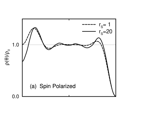
FIG. 3.: Mixed estimates of the density profiles of $\nu=1/3$ excited state wave functions on the sphere with a quasielectron at the top of the sphere $(\theta=0)$ and a quasihole on the bottom of the sphere $(\theta=\pi)$ with $r_{s}=1$ (dashed line) and $r_{s}=20$ (solid line), for (a) the spin-polarized excited state, and (b) the spin-reversed excited state. Results are for 20 electrons.

REFERENCES

- [1] J.M. Leinaas and J. Myrheim, Il Nuovo Cimento, 37B, 1, (1977); F. Wilczek, Phys. Rev. Lett. 48, 1144 (1982).
- [2] S.C. Zhang, T.H. Hansson, and S. Kivelson, Phys. Rev. Lett. 62, 82 (1989).
- [3] G. Ortiz, D.M. Ceperley, and R.M. Martin, Phys. Rev. Lett. 71, 2777 (1993).
- [4] P. J. Reynolds, D. M. Ceperley, B.J. Alder, and W. A. Lester, Jr., J. Chem. Phys. 77, 5593 (1982).
- [5] F.D.M. Haldane, Phys. Rev. Lett. 51, 605 (1983).
- [6] T. Chakraborty, P. Pietiläinen, and F.C. Zhang, Phys. Rev. Lett. 57, 130 (1986).
- [7] R. Morf and B.I. Halperin, Z. Phys. B 68 391 (1987).
- [8] F.C. Zhang and S. Das Sarma, Phys. Rev. B 33, 2903 (1986).
- [9] T.T. Wu and C.N. Yang, Nucl. Phys. B 107, 365 (1976).
- [10] J.K. Jain, Phys. Rev. Lett. 63, 199 (1989); Phys. Rev. B 40, 8079 (1989); ibid. 41, 7653 (1990).
- [11] V. Melik-Alaverdian, G. Ortiz, and N.E. Bonesteel, in preparation.
- [12] For a discussion of quantum corrections see, for example, B.S. DeWitt, Rev. Mod. Phys. 29, 377 (1957); and D.W. McLaughlin and L.S. Schulman, J. Math. Phys. 12 2520 (1971).
- [13] R. Price, P.M. Platzman, and S. He, Phys. Rev. Lett. 70, 339 (1993); R. Price and S. Das Sarma, Phys. Rev. B 54, 8033 (1996).
- [14] To reduce finite size effects we have followed [7] and quoted energies in units of where is a rescaled magnetic length.
- [15] N.E. Bonesteel, Phys. Rev. B 51, 9917 (1995).
- [16] R.L. Willet, H.L. Stormer, D.C. Tsui, A.C. Gossard, and J.H. English, Phys. Rev. B 37, 8476 (1988); For more recent measurements see R.R. Du et al., Phys. Rev. Lett. 70, 2944 (1993), and references therein.
- [17] H.C. Manoharan, M. Shayegan, and S.J. Klepper, Phys. Rev. Lett. 73, 3270 (1994).
- [18] D. Yoshioka, J. Phys. Soc. Jpn. 55, 885 (1986).
- [19] V. Melik-Alaverdian and N.E. Bonesteel, Phys. Rev. B 52, R17032 (1995).