Exact calculation of force networks in granular piles

Abstract

We present calculations of forces for two dimensional static sandpile models. Using a symbolic calculation software we obtain exact results for several different orientations of the lattice and for different types of supporting surfaces. The model is simple, supposing spherical, identical, rigid particles on a regular triangular lattice, without friction and with unilateral spring-like contacts. Special attention is given to the stress tensor and pressure on the base of the pile. We show that orientation of the lattice and the characteristics of the supporting surface have a strong influence on the physical properties of the pile. Our results agree well with numerical simulations done on similar systems and show, in some specific cases, a dip i.e. a depression under the apex of the pile. We also estimate that the algorithm we have developed can be easily adapted to other configurations and models of granulates and can be used in other physical cases where piecewise linear systems are encountered.

PACS Numbers: 46.10.+z, 46.30.Cn, 83.70.Fn, 07.05.Tp

I Introduction

Extensive interest has been devoted to the study of granular matter in the last few years [1]. It exhibits many surprising phenomena and even though classical mechanics is a mature domain, granulates in general, and static granular systems in particular still pose many open questions. In the case of a static heap of grains it was observed that the pressure on the supporting surface presents a local minimum (a dip) under the apex of the pile rather than the intuitively expected maximum [2, 3]. This observation is qualitatively explained by an arching effect, transporting the charge of the of the grains’ weight to the sides of the pile [4]. This idea was later incorporated in a new continuum approach [5, 6, 7, 8] under the so called “fixed principal axis” hypothesis model (FPA), in which the constitutive equation needed to close the system of equations states that the the stress tensor has its principal axis always pointing in the same direction. It is claimed that this characteristic is “remembered” by the grains from the moment they were buried at the surface of the pile when the pile has grown. This model gives results in very good agreement with the experimental data of 3D piles. The validity of this approach is not generally accepted, and some authors [9, 10] reject the basic assumption of the FPA model, pointing out that experiments on wedge form piles does not show any dip as predicted by the FPA model and that the FPA model cannot account for the observed sensitivity of the force networks in the heap to the base boundary conditions (see Ref. [9, 10] and references herein). It is claimed that the well known elasto-plastic continuum model of soils is still valid in the pile’s case. The dip, in this model is accounted by the existence of regions with different constitutive behaviors, plastic in the outer region and elastic in the inner region [11, 12].

Even though continuum models are very useful they do not give many clues about the micro-mechanical origin of the granular behavior, since these models are homogenized models taking a mean over a large number of grains. Some micromechanic models were proposed in order to link the grain-size physics to the pile-size phenomena [13, 14, 15, 16, 17, 18, 19, 20, 21]. One simple model is an array of rigid spheres arranged on a diamond lattice [15]. Under this kind of pile the normal force was shown to be constant even when periodic vacancies are introduced throughout the pile [17]. Varying the sizes of the grains or introducing attractive forces might change the forces under the pile, but still does not reproduce the experimental force profile [18].

Many of the discrete models used for granular matter use a large variety of numerical simulation techniques like molecular dynamics [21, 14], contact dynamics [22], cellular automata [19, 20] and others. Although these algorithms are useful in reproducing many of the characteristics of granular matter, none of these methods is completely satisfactory. Convergence is very slow due to the highly nonlinear character of the contact forces. The amplitude of forces in granular matter spawns several orders of magnitude [23, 1] producing badly conditioned numerical systems, and granular media are extremely sensitive to fluctuations [16, 24]. As a result, much care should be taken when numerically simulating granulates since cumulative roundoff errors might give rise to errors of considerable amplitude. Moreover, besides some very simple models [15, 17, 25], analytical results are uncommon for these discrete models so that numerical results are seldom verified.

A symbolic calculation software allows, in some cases, to perform numerical-like calculations while avoiding any numerical errors. When using such software one can perform automated analytical calculations as if they were done by hand but on systems of a size too large to be calculated by a human.

In this paper we present an implementation of such a calculation, in the case of a pyramidal piling of 2D discs, under the effect of gravity, and in the absence of friction. We use “spring-like” contacts under compression between discs and suppose them having infinite rigidity, solving the equilibrium equations in a straightforward way. We do not need any damping at the contacts, as it is often the case in numerical methods, since no dynamics is used in order to find the solution. Results obtained with this scheme are free of any numerical error.

We study a wide variety of geometrical configurations, with different supporting surfaces, lattice orientations and external constraints. In particular, some of the configurations proposed in Ref. [21], and studied using molecular dynamics, will be treated so to provide a cross check of numerical results.

The generality of this method makes it versatile and easily adaptable to other static cases like silo geometries, 3D pilings of spheres or the study of the force network under external mechanical constraints or any other case where piecewise linear equation systems are to be resolved.

The outline of the paper is the following: The model is exposed in Sec. II and the different configurations are listed in Sec. III. The algorithm is detailed in Sec. IV. Sec. V present the results for the different realizations that are discussed in Sec. VI.

II The model

Since we aim at getting exact results we must consider a simple model. First, we will consider only two dimensional piles formed of identical, frictionless, spherical grains (discs), of same radius $R$ and weight $w$. Those grains will be always arranged on a horizontal surface to form a pile on a triangular lattice, which is the natural lattice in this case. In this case the coordination number $n_{c}$ (the number of neighbors or the number of possible contacts) is greater than twice the space dimension so that if one only considers infinitely stiff discs, the system is hyperstatic i.e. the number of degrees of freedom in the system is bigger than the number of equations imposed by the mechanical equilibrium and the stability of the system $(\sum\vec{F}=0)$ is not sufficient to determine all forces. In such case, one must introduce new relations in order to close the problem.

The easiest way to introduce the necessary relations is to consider elastic, spring-like contacts between the discs, replacing the pile by an array of point-like masses linked by springs, so that the force applied by disc $d_{1}$ on disc $d_{2}$ is:

$$\vec{F}_{d_{1}\rightarrow d_{2}}=-\frac{1}{\tau}(2R-|\vec{r}_{d_{1}}-\vec{r}_{d_{2}}|)\,\frac{\vec{r}_{d_{1}}-\vec{r}_{d_{2}}}{|\vec{r}_{d_{1}}-\vec{r}_{d_{2}}|}\theta(2R-|\vec{r}_{d_{1}}-\vec{r}_{d_{2}}|)$$ (1)

where $\tau$ is the inverse of the elastic modulus (or the softness) of each disc-disc contact, and $\vec{r}_{d_{n}}$ the position of the disc $d_{n}$. $\theta$ represents the Heaviside step function. The $\theta$ functions are introduced in order to take into account the unilateral character of the contact forces in dry granular matter, i.e. that the discs can push (when $2R-|\vec{r}_{d_{1}}-\vec{r}_{d_{2}}|>0$) but not pull each other. The system is therefore non linear and clearly impossible to solve analytically, with or without the use of a symbolic calculation software, so some kind of simplifying assumption must be introduced. In particular, we consider the case of hard discs;

$$\tau\ll R/w$$ (2)

Since forces are finite, this condition implies that the displacements of the discs from the lattice points must tend to $0$ with $\tau$ , hence, when calculating to first order in $\tau$, these displacements are proportional to $\tau$. We can develop the equations to first order in all the displacements, linearizing the $(2R-|\vec{r}_{d_{1}}-\vec{r}_{d_{2}}|)\,\frac{\vec{r}_{d_{1}}-\vec{r}_{d_{2}}}{|\vec{r}_{d_{1}}-\vec{r}_{d_{2}}|}$ terms. The remaining non-linear parts involved are the $\theta$ functions that cannot be linearized around 0.

Dealing with the non-linearity arising from the $\theta$ function is the hardest part of the solution. One may consider calculating all possible combinations of absent/present contacts, solve the linear system obtained for each one of them and keep only solutions consistent with the conditions of the originally supposed contact network. Unfortunately, this method is extremely time consuming, since one must solve for $2^{c}$ different realizations, with $c$ the number of contacts in the system. We will deal with this difficulty by an iterative method described in Sec. IV.

Although we can use this algorithm for any value of $\tau$ so that $\tau\ll R/w$ (slightly deformable grains), in the following we will restrain ourselves to the case of rigid discs, taking (analytically) the limit $\tau\rightarrow 0$, in order to get results independent of $\tau$.

A question we did not address in this work, is the existence and uniqueness of the solution. Since the system of equations is non-linear both questions are open and deserve further investigation. We always found a solution for whatever pile size we studied, so that the existence is assured, at least for the pile sizes we have investigated.

III The geometrical configurations

We have studied the following geometrical configurations:

• A “tilted” triangular lattice pile with $30^{\circ}$ slope and the following surface conditions:

  • “bumpy” surface, as shown in Fig. 1. The pile poses on top of two layers of fixed discs; the centers of those discs are maintained on the triangular lattice points in order to simulate an infinitely rough surface. We will refer to this case as the TBS case (TBS for Tilted Bumpy Surface).

  • “smooth” flat surface with only the outermost base discs fixed, as shown in Fig. 2. In the following will refer to these discs as the corner stones. This case will be refered to as the TSS case. (TSS for Tilted Smooth Surface).

• A $60^{\circ}$ slope, “untilted” pile on a smooth surface, see Fig. 3. The NT60 case. (NT60 stands for Not Tilted 60 degrees slope) .

• A $30^{\circ}$ slope, “untilted” pile on a smooth surface, see Fig. 4, the NT30case. In this case we have studied the influence of applying a force on the lower row of discs by slightly displacing the corner stones. This configuration (amongst others) was studied in Ref. [21] using “spring-dashpot” contacts and solved with molecular dynamics.

IV The algorithm used

The algorithm was implemented on a Sun computer running Maple-V symbolic calculation software. Basically, the algorithm is looking for a configuration of the contacts for which the solution for the positions of the discs is compatible with all of Heaviside’s $\theta$ functions.

A simplified flowchart of this algorithm is shown in Fig. 6.

A Notations.

Here and below, we will use the following notations:

• The discs are indexed by the couple $(i,j)$ where $i$ is the row number, counting from the top to the bottom, and $j$ is the disc’s position counting from the left to right. See Fig. 1 for example.

• The forces that might act on the disc $(i,j)$ are named $a_{i,j},b_{i,j},c_{i,j},d_{i,j},e_{i,j},f_{i,j}$ and $p_{i,j}$. Note that the notations are different for the two lattice orientations and that $p_{i,j}$ is only present in the untilted case with smooth surface (see Fig. 5).

• We denote with $\alpha(i_{1},j_{1},i_{2},j_{2})$ the angle between the horizontal and the line connecting the centers of discs $(i_{1},j_{1})$ and $(i_{2},j_{2})$.

• We designate by $x_{i,j}$ and $y_{i,j}$ the $x$ and $y$ coordinates of the center of the disc $(i,j)$.

• We call $N$ the number of layers in the pile. In the bumpy surface case we consider $N$ as the number of free to move layers.

• We name $t_{i}$ the total number of discs on the $i$-th layer, $h_{i}$ the number of discs in one half of the $i$-th layer, center disc included and finally $h^{\prime}_{i}$ the same number but excluding the center disc. It is simple to see that:

  • For the tilted piles (Fig. 1 and 2) we have $t_{i}=i,\quad h_{i}=\left\lfloor\frac{i+1}{2}\right\rfloor$ and $h^{\prime}_{i}=\left\lfloor\frac{i}{2}\right\rfloor$.

  • For the $60^{\circ}$ slope untilted lattice pile (Fig. 3), $t_{i}=i,\quad h_{i}=\left\lfloor\frac{i+1}{2}\right\rfloor$ and $h^{\prime}_{i}=\left\lfloor\frac{i}{2}\right\rfloor$.

  • For the $30^{\circ}$ slope untilted lattice pile (Fig. 4), $t_{i}=3i-2,\quad h_{i}=\left\lfloor\frac{3i-2}{2}\right\rfloor$ and $h^{\prime}_{i}=\left\lfloor\frac{3i-1}{2}\right\rfloor$

• The variable $Z$ will contain, in our algorithm, the list of the forces between the couples of neighboring discs which are not in contact. These forces will be removed from the system of equations.

B Resolution steps

The general resolution steps are the following (see also the flowchart shown in Fig. 6):

1. Initialize $Z=\emptyset$. One can also start with another initial contact configuration closer to the solution in order to speed up the calculation time.

2. Write the system of equations $\sum\vec{F}_{i}=0$ for the entire pile for the $x$ and $y$ projections. In order to limit the size of the equation system we take immediately into account the $x\rightarrow-x$ symmetry of the pile. In other terms, we write only the projections on the $x$ axis of the equations for the discs $(i,j)$ with $i=1..N$ and $j=1..h^{\prime}_{i}$ and the projections on the $y$ axis for $j=1..h_{i}$. At the end of this step the system is written in terms of the forces $a_{i,j},b_{i,j},c_{i,j},d_{i,j},e_{i,j}$ (and eventually $p_{N,j}$) and the angles between the disc centers (see Fig. 5).

3. We introduce the conditions at the border and at the bottom of the pile. In other terms, substitute $0$ for forces like (in the TSS case) $b_{i,1},c_{i,1},e_{N-1,j}$ etc. where $i=1..N-1,j=1..t_{N-1}$.

4. We remove forces between neighbors not in contact. In other words, we substitute $0$ for all of the forces in the variable $Z$.

5. We apply Hook’s law (equation 1, replacing the $\theta$ functions by $1$), so that the forces are now expressed in terms of the positions of the centers of the discs.

6. Replace the angles by their expressions in the positions. For example, in the TSS and TBS case, pose:

   $$\cos(\alpha(i,j,i-1,j))=\frac{x_{i-1,j}-x_{i,j}}{\sqrt{(x_{i,j}-x_{i-1,j})^{2}+(y_{i,j}-y_{i-1,j})^{2}}}$$ (3)

7. At this point the equations are written entirely in terms of $x_{i,j}$ and $y_{i,j}$. The assumption of very high stiffness enters here, we rewrite the positions in terms of the displacements from the lattice points $\delta x_{i,j}$ and $\delta y_{i,j}$, i.e. we set $x_{i,j}=x^{lattice}_{i,j}+\delta x_{i,j}$ and $y_{i,j}=y^{lattice}_{i,j}+\delta y_{i,j}$.

8. We develop the equations to first order in those displacements.

9. We resolve the linear equations to find $\delta x_{i,j}$ and $\delta y_{i,j}$ . These displacements are proportional to $\tau$, the inverse elastic modulus.

10. In some cases (TSS, NT60, NT30) the system obtained in step 8 does not have any solution because too many forces were removed at once at the previous iteration and stability can no longer be assured. If such a case appears, we remove from $Z$ the force having the minimal value for $\left|2R-|\vec{r}_{i_{1},j_{1}}-\vec{r}_{i_{2},j_{2}}|\right|$, in other terms we reintroduce a contact between the closest couple of separated discs until equilibrium is regained.

11. Once the displacements are known, we use Hook’s law again in order to calculate the contact forces.

12. If some of those forces are found to be negative, i.e. the corresponding contact is attractive, we add them to $Z$ (those forces will be eliminated in step 4). In a similar manner, forces currently in $Z$ which are no longer attractive (since for the last solution found $2R-|\vec{r}_{i_{1},j_{1}}-\vec{r}_{i_{2},j_{2}}|\geq 0$), are removed from $Z$.

13. If the last step produced no change, we conclude that our solution satisfies all of Heaviside’s $\theta$ functions and the algorithm stops, returning the forces, $Z$ and the displacements. As we mentioned before this proves the existence of a solution, but there might be others. Otherwise, the list $Z$ is updated and the algorithm returns to step 2.

C Computer resources used

The computer time needed in order to get the final force configuration varied from some minutes (4 layers) to several days (more than 20 layers) on a Sparc 20 station. The maximum size varied from one configuration to the other, because some (like the TSS or NT30) needed more iterations than other cases before arriving to the correct contact configuration. Another limitation is memory, large systems create huge systems of equation that can occupy large amount of memory (we used up to 30Mb of RAM in some cases).

V Results

For each of the geometrical configurations we present several interesting characteristics derived from the solution:

  The force and contact networks:

When the algorithm stops, we obtain a contact network and its superposed force network. We will represent those networks in a single plot where a dashed line represents an absent contact, a full line represents a contact and it is drawn with a width proportional to the amplitude of the force. In some cases we observe the existence of a limit case where a contact exist but the force vanishes (osculatory discs). This kind of contacts will be represented by a dash-dot line. These plots will give us an idea of the effective lattice in different zones of the pile and the possible existence of an arching effect.

  The stress tensor:

The stress tensor $\sigma_{\alpha\beta}$, averaged over one particle and in the case of point-like contacts is given by:

$$\sigma_{\alpha\beta}=(1/V)\sum_{k}F_{\alpha}^{k}r_{\beta}^{k}$$ (4)

where the sum runs over all external forces acting on the particle, $F_{\alpha}^{k}$ is the $\alpha$-th component of the the $k$-th force, $r_{\beta}^{k}$ is the $\beta$-th component of its contact point position and $V=\pi R^{2}$ the volume of each particle. Since we neglect tangential forces the particles are torque free and the stress tensor is symmetric. In these plots, the stress tensor for each particle will be represented in by two segments of length proportional to the the eigenvalues and pointing at the direction of the eigenvectors (principal and secondary axis). The stress tensor will help us compare our results to results from various continuum mechanics approaches, especially to the fixed principal axis hypothesis.

  Pressure profile on the base of the pile:

The normal and (when present) horizontal forces applied by the pile on the supporting surface will be plotted as a function of the position $x$. These plots will provide a comparison of our results to the experimental data, mainly in order to verify whether a dip is present or not.

  Size dependency of the forces:

By solving for different pile sizes we can trace the evolution of the forces acting on a given disc as a function of the size of the pile. In order to get the maximum number of data points we concentrated on disc $(2,1)$.

A “Bumpy” surface tilted lattice : TBS

In this section we present the results for a piling of discs posed on 2 layers of discs attached to the lattice, as shown in Fig. 1.

1 The resulting force network

In this case one can notice that the missing contacts tend to appear on the flanks of the pile, while the in the inner part of the pile all neighboring discs are in contact. This behavior is incompatible with the basic FPA assumption since a particle at the open surface is in a completely different situation once it is buried. None of the contacts downwards are missing and we can notice that these contacts are the prefered paths for the forces thus excluding any arching.

2 The stress tensor

The resulting stress tensor is shown in Fig. 8. As we could expect, we do not observe in this geometry a fixed principal axis direction, but rather a typical result that would follow from the traditional IFE (Incipient Failure Everywhere) assumption (Ref. [7], Sec. 2.5). The stress tensors’ variations are quite smooth and all of the pile seems to have the same behavior.

3 The pressure profile

In the TBS case it is not straightforward to define uniquely the pressure or the normal force distribution on the supporting surface since it is in contact with two different layers. We show in Fig. 9 the normal and shear forces on the last layer of discs, ignoring those on the layer $N-1$. Because we took into account only the $N$-th layer the sum of the normal forces is smaller than the total weight of the pile. Anyhow, it is clear that the distribution does not show a dip but rather a maximum.

4 Dependence on the size of the pile

The evolution of the forces acting on the disc $(2,1)$ is plotted in Fig. 10. For small values of $N$, the finite size effects are large and the forces fluctuate considerably. But as the size increases, these effects disappear, and a linear regime is established. The important point here is that all the forces, even those at the top of the pile are highly correlated to the size and “feel” each added layer. We can expect that this should not be the case when the size of the pile gets even bigger and a saturation should occur. The question is how will it occur? Will asymptotically the forces tend to a constant value, or will they rather continue changing linearly until one of them (in the figure’s case $e_{2,1}$) will reach zero causing the corresponding contact to disappear and the other forces to stabilize? We are not able to study the behavior of the forces at the point where, for example, $e_{2,1}$ vanishes, since the computer resources needed would be too large for the corresponding pile sizes (more then 30 layers).

B Tilted lattice, smooth surface : TSS

The geometrical situation is presented in Fig. 2. Discs in the last row are free to move without friction on the surface, only the corner stones (in gray) are fixed on the lattice and are not allowed to move. This situation is technically harder than the previous one because on a bumpy surface the algorithm only removed contacts in every iteration without ever creating them again in the following iterations, so that every iteration approaches the final solution. Here, this is not the case. Contacts often reappear, making the approach to the final solution much slower.

1 Force network

An example of the force network obtained is shown in Fig. 11. This network differs considerably from the one in the TBS case. First of all the number of absent contacts is much larger and they appear mainly in the center of the pile and not just on the surface as in the TBS case. Secondly, a new case has appeared for which the force vanishes exactly, even though the corresponding contact does exist (osculatory discs). Again, nearly all of the vertical contacts are present so no arching is observed.

2 Stress tensor

The stress tensors’ principal and secondary axis are shown in Fig. 12. Again, the results differ from the TBS case. We can observe 3 regions with different behaviors with an abrupt transition:

• Discs on the surface of the pile, having the principal axis pointing along the surface.

• Discs in the inner part of the pile, having the principal and secondary axis pointing horizontally or vertically.

• Discs at the shoulders of the pile with no clear prefered direction.

In this case our result is in contradiction to the basic assumption of the FPA model since the stress tensor on the surface of the pile differs considerably from the one of a buried particle.

3 Pressure profile

The normal forces acting on the surface of a 13 layer pile are shown in Fig. 13. The shear force acting on the bottom layer is zero because of the smoothness of the surface. This pressure profile is close to the one in the TBS case displayed in Fig. 9. As in the TBS case we do not observe a dip but rather a maximum.

4 Variations of the forces with the size of the pile

The variations of forces acting on disc $(2,1)$ are presented in Fig. 14 (compare with Fig. 10). We observe a strong dependence on the parity of $N$ and a saturation of the forces for large pile sizes of the same parity. We do not have enough data in order to determine whether the dependence on the parity of $N$ continues for even larger piles.

C The NT60case: “untilted” lattice, $60^{\circ}$ slope pile

The system in this case is shown in Fig. 3. When one does not consider the horizontal contacts (equivalent to taking a slope slightly inferior to $60^{\circ}$) it is easy to calculate analytically the forces and find that the distribution of normal forces is uniform on the base and that the shear force on the base varies linearly with the position [15, 17, 25]. In this case we always get a contact network in which all horizontal contacts are absent, thus giving the same solution as the one in Ref. [15]. This gives us another verification for our method and an indication about the uniqueness of the solution. Numerical calculations give the same effect [21].

D The NT30case: “untilted” lattice, $30^{\circ}$ slope pile

The configuration in this case is the one shown in Fig. 4. Like in the TSS case, we fix the corner stones in order to keep the heap stable. This particular geometry was proposed (amongst others, not studied here) in Ref. [21], and studied by numerical simulation using the molecular dynamics method. Since in this kind of pile the number of discs grows faster with the number of layers than in the previous configurations, we were only able to calculate the force network for piles having less than 7 layers, making a systematic size effect study impossible.

1 The force network

An example of the force network obtained in this case is shown in Fig. 15. We notice 3 regions somewhat similar to those observed in the TSS case (see Sec. V B 1 and Fig. 11). Only at the outermost parts of the pile traces of arching are seen where some contacts downwards are absent. In the central part of the pile all of the horizontal contacts are absent, and between those two zones all contacts are present. In Fig. 16 we show numerical results obtained by molecular dynamics and provided by Luding [26, 21] for the same pile. They show excellent agreement with ours, even though the numerical results present some differences (some contacts that are absent and should be present or the vice versa) and imperfections (notice that the numerical force network is not exactly symmetric especially at the corner stones).

2 The stress tensor

The stress tensor in this case, shown in Fig. 17, is quite similar to the one obtained for the TBS pile (see Fig. 8), and no FPA is observed. For comparison, results from Ref. [26, 21] are superposed (represented by ellipses). The agreement is so good that the plots are hardly distinguishable.

3 The pressure profile

The pressure profiles for a 5 layer pile (dashed line) and a 6 layer pile (full line) are shown in Fig. 18. Both present a plateau and a shallow minimum under the apex of the pile or near it. We also observe a small depression at the shoulders of the pile that, as we will see in Sec. V D 4, will play an important role when the corner stones are pushed in. We also plot on the same figure results from Ref. [26, 21] (in circles) that, again, agree well with ours.

4 The effect of displacing the corner stones

Another point studied in Ref. [21] is the effect of horizontally pushing or pulling the corner stones on the bottom layer. It was observed that pushing in those discs, i.e. fixing their position on the a position slightly closer to the axis of the pile, causes the pressure distribution on the base to present a deeper dip than the one observed without it.

We studied the same problem using an exact symbolic algorithm which is an extension of the previous one. Since all calculations are done to the first order in $\tau$ we should only consider displacements proportional to $\tau$ i.e. $\delta x_{N,1}=q\tau$ and $\delta x_{N,t_{N}}=-q\tau$, otherwise the resulting forces will be infinite.

To find the correct contact configuration for a given value of the parameter $q$, namely $q_{end}$ we proceed in the following way:

  

1. We apply the algorithm described in Sec. IV B in order to solve for $q=0$.

  

2. For the contact network obtained in step 1 and for an arbitrary $q$ we find the distance between every couple of neighboring discs : $d_{i,j}(q)$ to first order in $\tau$. Those distances depend on $q$ linearly, so we can write : $d_{i,j}(q)=\alpha_{i,j}q+\beta_{i,j}$.

  

3. We solve all the equations $d_{i,j}(q)=2R$ for $q$. When a solution exists it is unique, we denote it $q^{\prime}_{i,j}$. In other terms, $q^{\prime}_{i,j}$ are the values of $q$ where the contact network might change, i.e. contacts might disappear or reappear.

  

4. We calculate;

$$q^{\prime\prime}=\left\{\begin{array}[]{ll}\min(q^{\prime}_{i,j}|(q^{\prime}_{i,j}>q)&\hbox{if }q_{end}>0\\ \max(q^{\prime}_{i,j}|q^{\prime}_{i,j}<q)&\hbox{if }q_{end}<0\end{array}\right.$$ (5)

In practice, we find the next $q$ for which the contact network might change.

  

5. If $|q^{\prime\prime}|>|q_{end}|$ then no change in the contact network will happen between $q$ and $q^{\prime\prime}$ and since the network and $d_{i,j}(q)$ are known for this interval of values, and hence for $q=q_{end}$, we can calculate the forces for $q=q_{end}$ easily from equation (1) and the algorithm stops.

The expression of each force, as a function of the positions, is continuous around $q^{\prime\prime}$ (equation 1) so that no discontinuity can occur in the forces if contacts having $d_{i,j}(q^{\prime\prime})=2R$ disappear, only $\alpha_{i,j}=dd_{i,j}(q)/dq$ might be modified.

  

6. We modify the contact network to take into account the changes supposed to take place at $q^{\prime\prime}$. We set $q=q^{\prime\prime}$ and jump back to step 2.

  

7. In some cases the modification we applied to the contact network must be reviewed since in certain cases a force $F_{i,j}$ vanished in $q^{\prime\prime}$ but $\hbox{sign}(\alpha_{i.j}(|q|<|q^{\prime\prime}|))=-\hbox{sign}(\alpha_{i.j}(|q|>|q^{\prime\prime}|))$ so that the corresponding contact should not change. For example, two neighboring discs that were approaching one another for $q<q^{\prime\prime}$ i.e. $\left.\alpha_{i,j}\right|_{q\rightarrow q^{\prime\prime+}}<0$ and for which $d_{i,j}(q^{\prime\prime})=2R$ will be supposed in contact in the new network, but if $\left.\alpha_{i,j}\right|_{q\rightarrow q^{\prime\prime-}}>0$ this contact should not reappear. When the algorithm detects such cases the contact network is corrected.

An example for results of the implementation of this method is shown in Fig. 19 and the variations of the normal forces on the supporting surface are shown in Fig. 20. The values of $q$ where the contact network rearranges for the 6 layer pile are given in table I. We observe several interesting points in this case. The initial pile is insensitive to positive values of $q$, in other terms no change in the force network appears when the corner stones are pulled apart. This appears to be a characteristic of the solution for all lattice orientations when the surface is smooth (not exposed here). On the contrary, when pushing the corner stones together $(q<0)$ the network is restructured at many values of $q$ (table I). The number of those values is finite so that for large values of $-q$ the contact network no longer changes. At this point (see Fig. 19) the network is characterized by a large number of absent vertical contacts and all of horizontally neighboring discs in contact, which is exactly what one might classify as an arching effect. As observed in Ref. [21] the arching is accompanied by the appearance of a pronounced depression under the apex and a FPA situation. We were able to calculate the exact evolution of the pressure under the apex of the pile as a function of $q$, see Fig. 20. For large values of $-q$ the pressure under the apex of the pile is decreasing with $-q$ until it reaches its asymptotic value. Surprisingly, we also observe a region for small values of $-q$ for which the minimum is less pronounced and even becomes a maximum (see the third frame in Fig. 19). The mechanism of the this change can be understood from Fig. 19. It is not the small depression under the apex of the pile, observed for $q=0$, that is the source for the dip when $-q$ is big, but rather the depressions observed at the flanks of the pile. These depressions move toward the center to create the dip.

VI Conclusions

In this paper we have presented an approach capable of producing exact results for the force and contact networks for piles of regularly packed hard discs for a large variety of cases: different orientations, geometries and supporting surfaces. The advantage of this method is that results are completely reliable since they a free of roundoff or other numerical errors. We obtain a wide variety of results for the different realizations we study. We conclude that lattice orientation and the characteristics of the supporting surface have a very important impact on the physical properties of the pile even when the pile is globally the same, and the contacts are of the same nature. Permitting propagation of forces vertically downwards when using a “tilted” lattice (TBS and TSS cases) leads to a behavior completely contrary to arching where the contact forces of the largest amplitude are vertical. On the other hand, when no vertical propagation is possible arching is more likely to occur, like we notice in the “untilted” case NT30. Arching can also be stimulated by imposing external constraints on the system that favor the horizontal contacts, like pushing in the corner stones. We were able to follow step by step the reorganization of the contact network while the pile is increasingly controlled by arching and a dip is established as the constraints grow. Experimental evidence for the importance of the orientation of the lattice of 2D granular systems was already observed for dynamic systems [27], but is generally ignored for static systems where the “untilted” lattice is the one generally used. Since real granular systems are disordered, real effects should not depend on the local orientation of the lattice. Much care should be taken when interpreting results that do depend on the orientation.

We confirm the claims in Ref. [9] about the sensitivity of the results to the boundary conditions at the base of the pile, especially the roughness of the surface has a large influence on both the contact network and the stress tensor (compare Fig. 7 to 11 and 8 to 12).

The results we get with this method can be used to check the precision of widely used numerical simulations, for much larger systems. We were able to do so in the NT30 case producing the same results as in Ref. [21]. We also confirm the effect that pushing the corner stones have on the pressure profile i.e. the dip becoming pronounced.

On the other hand, we do not get comparable results when pulling out the corner stones. In Ref. [21] asymmetric solutions were obtained in this case, and might indicate the existence of more than one solution or of a numerical flaw. We do not observe any rearrangement of the contacts when the corner stones are pulled apart, which seems to be a characteristic of all solutions with $q=0$. One must keep in mind, however, that in Ref. [21] results are given for a finite value of the stiffness, while here the stiffness is infinite.

In the NT30case, (Fig. 18) the pressure on the base of the pile presents, for an even number of layers, the famous dip observed under the apex of granular heaps [2, 3].

We also observe, as in Ref. [21] that the dip becomes more pronounced as we increase the applied force on the corner stones, but we also conclude that this dip is not formed by deepening of the shallow minimum observed for $q=0$ but rather from the small depressions at the flanks that move toward the center of the pile when $-q$ increases.

However, in light of the discussion above, concerning the sensitivity of results to the type of supporting surface and lattice orientation, and since a dip was not observed for the “tilted” piles (Fig. 9 and 13), we believe that one cannot conclude that this simple model contains the physical ingredients that give rise to the depression under the apex of the pile or to the FPA situation.

The method we used can be easily adapted to other geometries like silos or 3D pilings of spheres. One might also consider the introduction of other physical ingredients like friction or polydisperse disc sizes. The introduction of friction doubles the number of degrees of freedom of the system, since tangential components of the contact forces are added to each of the contact forces. On the other hand Coulomb’s friction law does only supply us with an inequality $F_{||}\leq\mu F_{\perp}$ rather than an equality. One can face this problem in two ways:

• Use the inequality solving facility in Maple in order to get bounds to the force values. This would probably be a difficult task mainly because of the $\theta$ functions.

• Introduce a supplementary assumption about the friction forces like $F_{||}=\mu F_{\perp}$ which is the IFE assumption, or any other relation between the forces.

The introduction of disorder into the system (polydisperse grains) does not present conceptual problems and could be faced in principle in the framework of our approach. However, it would be hard , in this case, to get reliable statistics due to the long resolution times.

VII Acknowledgments

We would like to thank Stéphane Roux for enlightening discussions, Loïc Sorbier for his work on the $q$ algorithm and Reuven Zeitak for a fruitful discussion on the $q$ algorithm.

Bibliography

Tables

$$\begin{array}[]{|rl|rl|rl|}\hline\cr&&&&&\\ {\displaystyle q_{1}=}&{\displaystyle-\frac{64757787245}{13047053469}\,\sqrt{3}}&{\displaystyle q_{2}=}&{\displaystyle-\frac{61636606607}{11780554266}\,\sqrt{3}}&{\displaystyle q_{3}=}&{\displaystyle-\frac{762822774179}{132529054821}\,\sqrt{3}}\\ &&&&&\\ {\displaystyle q_{4}=}&{\displaystyle-\frac{6707882705971}{1062824475948}\,\sqrt{3}}&{\displaystyle q_{5}=}&{\displaystyle-\frac{4445792285474}{687757544473}\,\sqrt{3}}&{\displaystyle q_{6}=}&{\displaystyle-\frac{2397551418033037}{365699270454792}\,\sqrt{3}}\\ &&&&&\\ {\displaystyle q_{7}=}&{\displaystyle-\frac{892376842807618}{118456895286735}\,\sqrt{3}}&{\displaystyle q_{8}=}&{\displaystyle-\frac{1040529221853421}{136826565791760}\,\sqrt{3}}&{\displaystyle q_{9}=}&{\displaystyle-{\frac{10760229006102401}{1372821783991152}}\,\sqrt{3}}\\ &&&&&\\ {\displaystyle q_{10}=}&{\displaystyle-{\frac{688471809160333}{83961109063488}}\,\sqrt{3}}&{\displaystyle q_{11}=}&{\displaystyle-{\frac{8424287631067}{527998087996}}\,\sqrt{3}}&{\displaystyle q_{12}=}&{\displaystyle-{\frac{23088074878561}{1393226957796}}\,\sqrt{3}}\\ &&&&&\\ {\displaystyle q_{13}=}&{\displaystyle-{\frac{203779480235}{10761198684}}\,\sqrt{3}}&{\displaystyle q_{14}=}&{\displaystyle-{\frac{54690800571}{2080923200}}\,\sqrt{3}}&{\displaystyle q_{15}=}&{\displaystyle-{\frac{122907611189}{3605129400}}\,\sqrt{3}}\\ &&&&&\\ {\displaystyle q_{16}=}&{\displaystyle-{\frac{13899925451}{389467512}}\,\sqrt{3}}&{\displaystyle q_{17}=}&{\displaystyle-{\frac{8553278999}{235721424}}\,\sqrt{3}}&{\displaystyle q_{18}=}&{\displaystyle-{\frac{258704085}{6896912}}\,\sqrt{3}}\\ &&&&&\\ {\displaystyle q_{19}=}&{\displaystyle-{\frac{15648333}{325196}}\,\sqrt{3}}&{\displaystyle q_{20}=}&{\displaystyle-{\frac{35529}{704}}\,\sqrt{3}}&{\displaystyle q_{21}=}&{\displaystyle-{\frac{199011}{3136}}\,\sqrt{3}}\\ &&&&&\\ {\displaystyle q_{22}=}&{\displaystyle-{\frac{2209}{33}}\,\sqrt{3}}&{\displaystyle q_{23}=}&{\displaystyle-{\frac{266}{3}}\,\sqrt{3}}&&\\ &&&&&\\ \hline\cr\end{array}$$

TABLE I.: Values of the parameter $q$ for which the contact network rearranges in the NT30 case for a 6 layer pile.

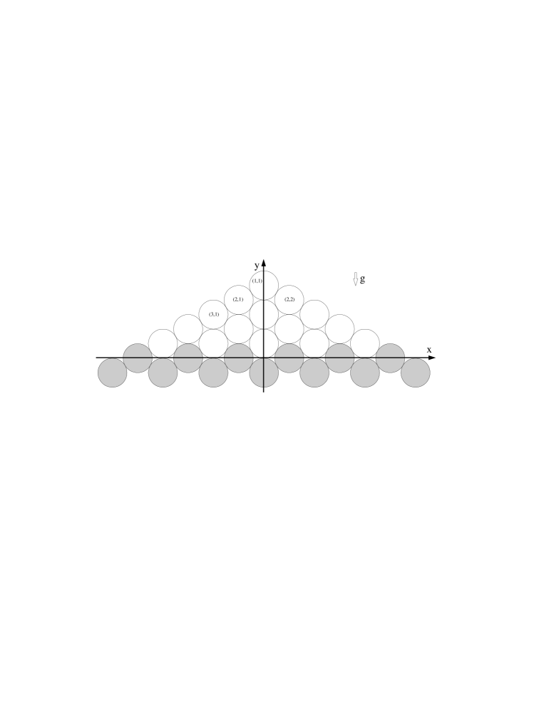
FIG. 1.: A “tilted” triangular lattice pile of 5 layers (TBS case) with a slope of $30^{\circ}$, the 2 gray layers represent the “bumpy” floor. Those two layers have their centers fixed on the lattice points. The indexing convention $(i,j)$ used is shown.

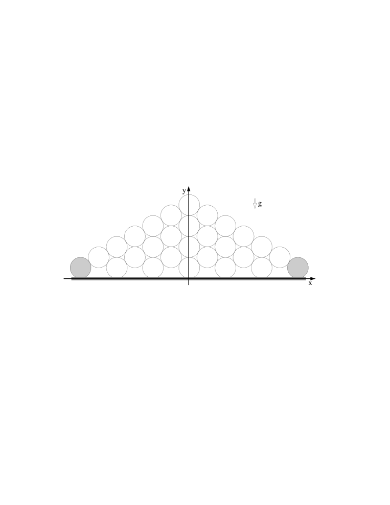
FIG. 2.: A “tilted” triangular lattice pile of 7 layers (TSS case) with a slope of $30^{\circ}$, the 2 gray discs (corner stones) have their centers fixed on the lattice points.

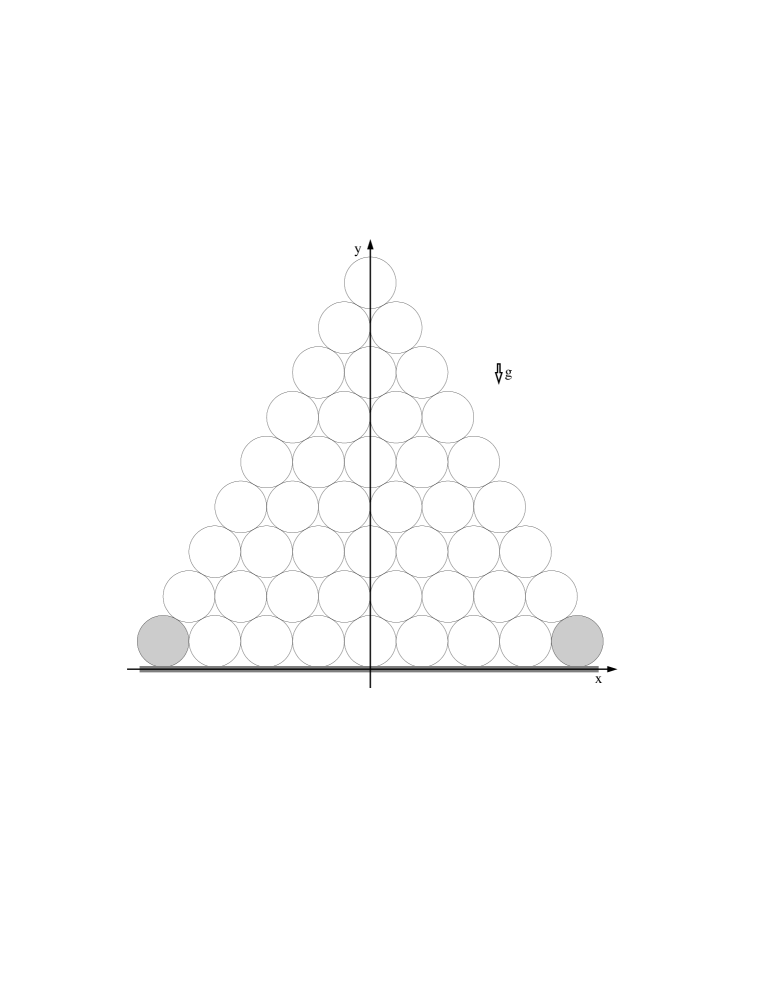
FIG. 3.: A triangular lattice pile of 9 layers in the NT60 case, the 2 gray discs (corner stones) are fixed on the lattice points.

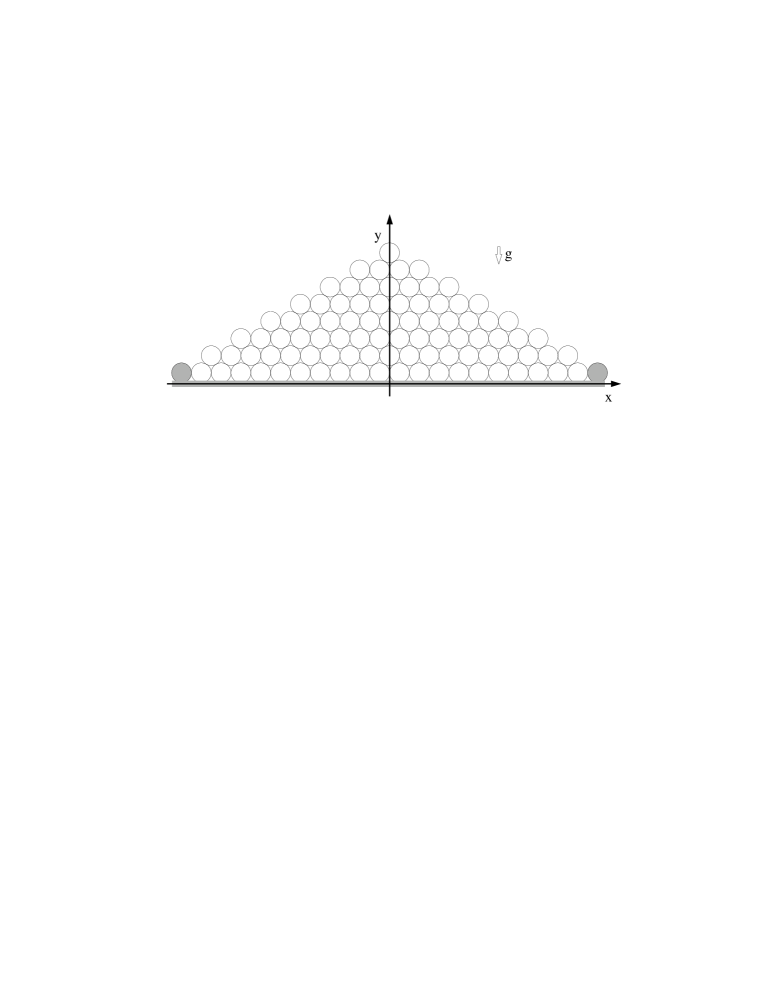
FIG. 4.: A triangular lattice pile of 8 layers with $30^{\circ}$ slope (the NT30 case), the 2 gray discs (corners stones) are fixed on the lattice points.

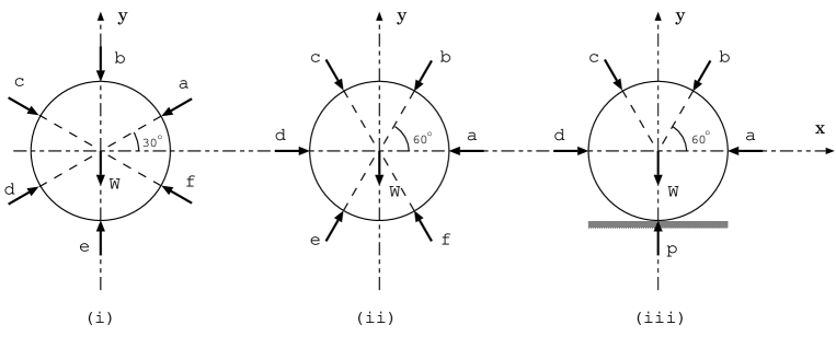
FIG. 5.: The notations used for the forces names. (i) represents the case of a tilted lattice (TBS and TSS cases), (ii) and (iii) represents the untilted one (NT60 and NT30), where (ii) is the case of a disc in one of the upper $N-1$ layers and (iii) is the case of discs that touch the surface. The angles are those for the limit $\tau\rightarrow 0$.

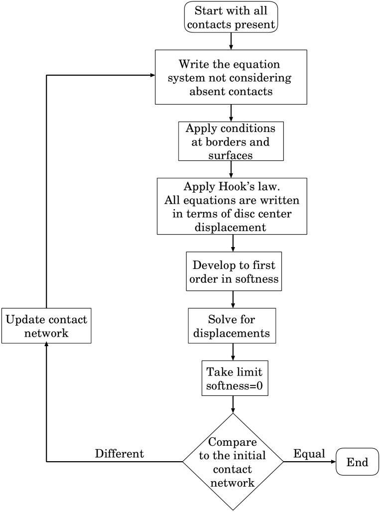
FIG. 6.: A simplified flowchart of the resolution algorithm used (see Sec. IV for more details).

FIG. 7.: The force network for a pile of 15 layers in the TBS case. The line width is proportional to the force amplitude, the dashed lines represent absent contacts (see Sec. V for more details).

FIG. 8.: The principal and secondary axis of the stress tensor for a pile of 11 layers for the TBS case (see Sec. V for more details).

FIG. 9.: The normal (full line) and shear (dashed line) forces on the base of a pile of 17 layers in the TBS case. We do not observe any dip in the normal force distribution. The shear forces vanish at the center of the pile as expected from symmetry (see Sec. V for more details).

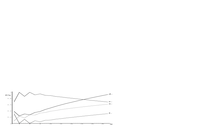
FIG. 10.: The dependence of the forces acting on disc (2,1) on the size of the pile for the TBS case. $N$ is the number of layers, a,d,e and f are forces acting on the disc as defined in figure 5. All forces are normalized by a disc weight (see Sec. V for more details).

FIG. 11.: The force network of a pile of 10 layers in the TSS case (see Sec. V for more details).

FIG. 12.: Principal and secondary axis of the stress tensor in a pile of 10 layers for the TSS case (see Sec. V for more details).

FIG. 13.: Pressure profile on the base of a 13 layers TSS pile (see Sec. V for more details).

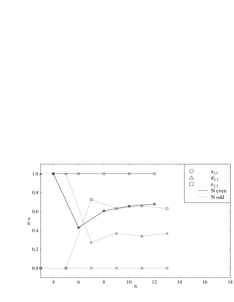
FIG. 14.: Variation of the different forces acting on the disc $(2,1)$ as a function of the size of the pile measured in layers; $N$, in the TSS case. For clarity $f_{2,1}$ is not shown since we obtain for all sizes that $f_{2,1}=1-e_{2,1}$. Notice the dependence in the parity of $N$ that stays pronounced even for large $N$ (see Sec. V for more details).

FIG. 15.: Force network in the NT30 case for a 6 layer pile (see Sec. V for more details).

FIG. 16.: The force network obtained for the NT30 case by molecular dynamics simulation of a pile of 6 layers [26].

FIG. 17.: The principal and secondary axis in the NT30 case for a 6 layer pile (in the cross representation) and a comparison to results obtained in Ref. [21] (represented by ellipses). Notice the excellent agreement between the two (see Sec. V for more details).

FIG. 18.: The normal pressure profile for the NT30 case for a 5 (dashed line) and 6 (full line) layer pile. For the 6 layer pile we obtain a small dip below the apex of the pile (see Sec. V for more details).

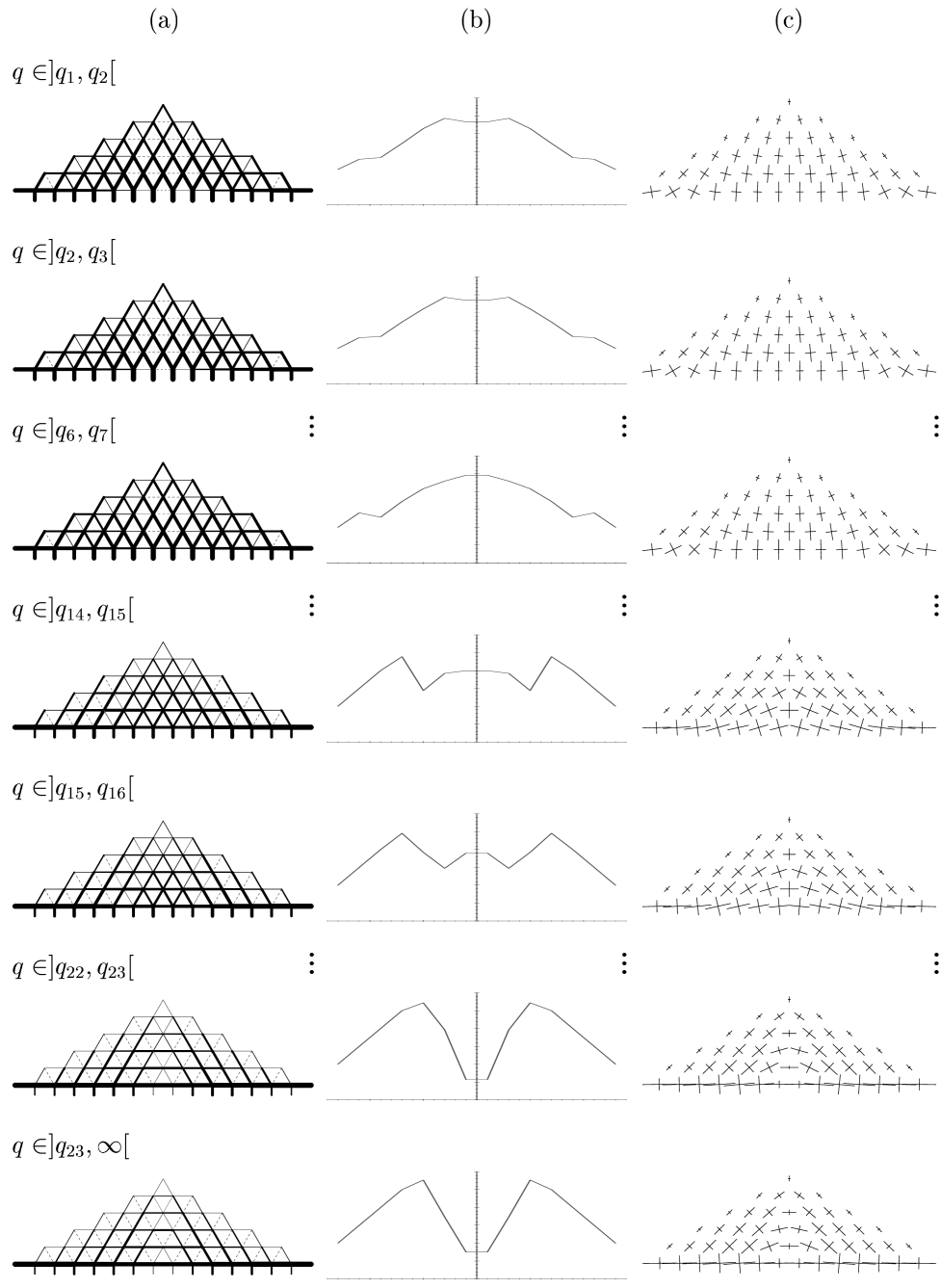
FIG. 19.: The changes in the force network (a), pressure profile (b) and the stress tensor (c) for growing values of $-q$ (see table (I) for the values of $q_{i}$) for a 6 layer NT30 pile. In column (b) the abscissa represents the $x$ axis, and varies between $-14$ and $14$ in disc radii unit, and the ordinate represents the force measured in disc weights $F/w$ varying in the range $0$ to $6$. The length of the representation of the principal axis of the stress tensor (c) and the width of the lines in the force network plots (a) are in a logarithmic scale.

FIG. 20.: Variation of the pressure under the apex of the pile with $q$ in the NT30 case. The dots represent the values of $q$ where the contact network rearranges (see table I).

Bibliography

\@afterheading
- [1] H. M. Jaeger, S. R. Nagel, and R. P. Behringer, Physics Today 49, 32 (1996).
- [2] J. Šmíd and J. Novosad, I.Chem. E. Symposium Series 63, D3/V/1 (1981).
- [3] B. Brockbank, J. Huntley, and R. Ball, Journal de Physique II 7, 1521 (1997).
- [4] S. F. Edwards and C. C. Mounfield, Physica A 226, 25 (1996).
- [5] J.-P. Bouchaud, M. Cates, J. R. Prakash, and S. Edwards, Phys. Rev. Lett. 74, 1982 (1995).
- [6] J.-P. Bouchaud, M. Cates, and P. Claudin, J.Phys.I 5, 639 (1995).
- [7] J. Wittmer, M. Cates, and P. Claudin, J. Phys. I 7, 39 (1997).
- [8] J. Bouchaud, P. Claudin, M. Cates, and J. Wittmer, in Physics of Dry Granular Media, proceedings of the cargèse summer school, edited by H. Herrmann, J.-P. Hovi, and S. Luding (Kluwer Academic Publishers, The Netherlands, 1998), pp. 97–122.
- [9] S. B. Savage, in Powders & Grains 97, edited by R. P. Behringer and J. T. Jenkins (Balkema, Rotterdam, 1997), pp. 185–194.
- [10] S. Savage, in Physics of Dry Granular Media, proceedings of the cargèse summer school, edited by H. Herrmann, J.-P. Hovi, and S. Luding (Kluwer Academic Publishers, The Netherlands, 1998), pp. 25–96.
- [11] F. Cantelaube and J. Goddard, in Powders & Grains 97, edited by R. P. Behringer and J. T. Jenkins (Balkema, Rotterdam, 1997), p. 231.
- [12] F. Cantelaube, A. Didwania, and J. Goddard, in Physics of Dry Granular Media, proceedings of the cargèse summer school, edited by H. Herrmann, J.-P. Hovi, and S. Luding (Kluwer Academic Publishers, The Netherlands, 1998), pp. 123–128.
- [13] D. Stauffer, H. Herrmann, and S. Roux, J. de Physique 48, 247 (1987).
- [14] K. Liffman, D. Chan, and B. Hughes, Powder Technology 72, 255 (1992).
- [15] D. Hong, Phys. Rev. E 47, 760 (1993).
- [16] P. Claudin and J.-P. Bouchaud, Phys. Rev. Lett. 78, 231 (1997).
- [17] J. Huntley, Phys. Rev. E 48, 4099 (1993).
- [18] K. Liffman, D. Chan, and B. Hughes, Powder Technology 78, 263 (1994).
- [19] J. Hemmingsson, Physica A 230, 329 (1995).
- [20] J. Hemmingsson, H. J. Herrmann, and S. Roux, J. Phys. I 7, 291 (1997).
- [21] S. Luding, Phys. Rev. E 55, 4720 (1997).
- [22] F. Radjai, M. Jean, J. J. Moreau, and S. Roux, Phys. Rev. Lett. 77, 274 (1996).
- [23] C. Liu et al., Science 269, 513 (1995).
- [24] E. Clément, C. Eloy, J. Rajchenbach, and J. Duran, in Lectures on stochastic dynamics, edited by T. Pöschel and L. Schimanski-Geier (Springer Verlag, Berlin, 1997).
- [25] M. K. H. Menon, in Non-linearity and breakdown in soft condensed matter, proceedings, Calcutta, India (Springer-Verlag, Heidelberg, FRG, 1993), pp. 40–46.
- [26] S. Luding, private communication.
- [27] J. Duran, T. Mazozi, E. Clément, and J. Rajchenbach, Phys. Rev. E 50, 3092 (1994).