[

Network of edge states: random Josephson junction array description

Abstract

We construct a generalization of the Chalker-Coddington network model to the case of fractional quantum Hall effect, which describes the tunneling between multiple chiral edges. We derive exact local and global duality symmetries of this model, and show that its infrared properties are identical to those of disordered planar Josephson junction array (JJA) in a weak magnetic field, which implies the same universality class. The zero frequency Hall resistance of the system, which was expressed through exact correlators of the tunneling fields, is shown to be quantized both in the quantum Hall limit and in the limit of perfect Hall insulator.

]

The QH transitions[1] provide one of the best testing grounds for our understanding of quantum critical phenomena. The main advantages of this system are the availability of well-controlled samples, and the variety of field and gate-voltage-driven transitions within one sample. Unfortunately, it appears that current theoretical understanding of the bulk QH effect is lagging behind the variety of experimentally observed features. Not only the transitions are found[2, 3] to have universal scaling exponents and universal critical conductances[3, 4] as suggested[5] basing on the bosonic Chern-Simons (CS) model[6], but their $I$–$V$ traces at different filling fractions appear to be algebraically related in a surprisingly wide range of parameters. Most notable are the reflection symmetry[7] of $I$–$V$ traces, and the quantized Hall insulator[4, 8] (QHI) phenomenon.

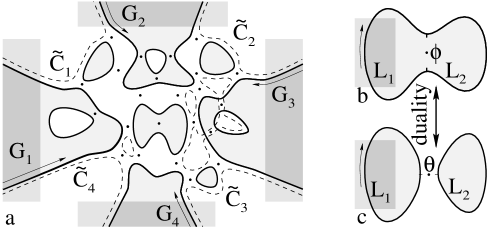
FIG. 1.: Left: An illustration of the chiral edge network. Only the tunneling phases in saddle points (solid dots) remain in the effective tunneling model. Four-point measurement can be performed via the external gates $G_{n}$ coupled to long leads. Dashed lines outline some of the dual edges $\tilde{\cal C}_{n}$. Right: The simplest example of the finite-system duality between a QH droplet with a backscattering point and two separate droplets connected by a tunneling point.

Theoretically, despite the attempted[9] rigorous analysis of the bulk CS model, the suggested universality[5] of the QH transitions has not been proven beyond the RPA. It was argued[10] that both the charge-vortex duality and the QHI phenomenon (the semicircle law[11]) must be present simultaneously to account for the observed symmetry of $I$–$V$ traces. Although the derivation of the semicircle law implies a duality between macroscopic current density and electric field, so far there was no quantum model to demonstrate both properties. Note, however, that the network of chiral edges, illustrated in Fig. 1a, shows both the correct scaling behavior (integer regime, Chalker & Coddington[12]), and the QHI phenomenon (high temperatures, Auerbach & Shimshoni[13]). Moreover, the effective action for a single tunneling junction has an exact dual representation[14, 15]. An important question is whether these features hold for the network of fractional edges at small temperatures.

The goal of this letter is to construct the tunneling action for the network of chiral edge states. We derive local and global duality symmetries of the partition function, and show that the infrared properties of the system are identical to those of the disordered JJA in a weak magnetic field, which implies the same universality class. We also express the four-point resistance of this system through exact correlators of the tunneling fields.

Gapless edge excitations $u\equiv u(x,\tau)$ in the QH regime are described[16] by the imaginary-time action

$$S_{0}=\frac{1}{4\pi}\int{u^{\prime}(i\dot{u}+vu^{\prime})}dx\,d\tau,$$ (1)

in our units the edge wave velocity $v\!=\!1$. The action remains quadratic[16, 17] in the presence of Coulomb forces; the interaction is introduced by the tunneling

$$S_{t}=\sum_{i<j\leq 2N}\int d\tau\sum_{k=1}^{\infty}\lambda_{ij}^{(k)}\cos(gk\phi_{ij}),$$ (2)

where $g\!=\!\sqrt{\nu}$ for the quasiparticles’ tunneling between the points $x_{i}$ and $x_{j}$ through the condensate with the filling fraction $\nu\!=\!(2m+1)^{-1}$, or $g\!\rightarrow\!\tilde{g}=1/\sqrt{\nu}$ for tunneling of electrons through an insulating region. The tunneling amplitudes $\lambda_{ij}^{(k)}$, set by the details[19] of the self-consistent potential near saddle points $\alpha\equiv{ij}$, $1\!<\!\alpha\!\leq\!N$ are treated as phenomenological parameters. Although the argument of the cosine in Eq. 2 is usually written as the difference $\phi_{ij}\!=\!u_{j}\!-\!u_{i}$, we must remember that tunneling connects two separate points, and there may be an additional gauge field contribution[18].

The non-linear action (2) depends on values $u_{i}$ of field $u$ in a discrete set of points $x_{i}$; its fluctuations in all other points can be integrated out. Leaving the arguments $\phi_{\alpha}$ of the tunneling terms as the only independent variables (cf. gauge-invariant phases for Josephson junctions), we write the most general form of the tunneling action

$$S[\phi_{\alpha}]=T\sum_{\omega=2\pi nT}{\omega\over 4\pi}\bar{\phi}_{\alpha}K_{\alpha\beta}\phi_{\beta}+S_{t},$$ (3)

with Matsubara frequencies $\omega$ and $\bar{\phi}_{\alpha}(\omega)\equiv\phi_{\alpha}(-\omega)$. Different tunneling points are linked by the elements of the coupling matrix $K_{\alpha\beta}(\omega)=-K_{\beta\alpha}(-\omega)$, determined by the geometry of edge channels; the factor $\omega/4\pi$ was separated for notational convenience.

Before specifying the form of the coupling matrix $K$, let us discuss general properties of the action (3):
(i) In the absence of any tunneling the matrix $K$ is uniquely determined by correlators of the fields $\phi_{\alpha}$,

$$\bigl{(}K^{-1}\bigr{)}_{\alpha\beta}={\textstyle{\omega\over 2\pi}}\left\langle\phi_{\alpha}\bar{\phi}_{\beta}\right\rangle_{\lambda=0}.$$ (4)

Therefore, the matrix elements between the tunneling points located at otherwise disconnected edges vanish. (ii) In the limit of infinite frequencies, the coherence between different tunneling points is also lost, while the matrix $K$ acquires its asymptotic form

$$K_{\alpha\beta}(\omega)\stackrel{{\scriptstyle\omega\rightarrow\infty}}{{\longrightarrow}}\delta_{\alpha\beta}\,{\rm sgn}\,(\omega)$$ (5)

(iii) The action (3) describes a complicated system of non-linear damped anharmonic oscillators. Since their mutual coupling is linear, each of these oscillators may be regarded as a particle

$$S_{1}={{T\over 4\pi}}\sum_{\omega}\omega\bigl{[}K_{11}(\omega)|\phi_{1}|^{2}+V_{1}\bar{\phi}_{1}-\phi_{1}\bar{V}_{1}\bigr{]}+S_{t}[\phi_{1}],$$

in its own periodic potential and external field $V_{1}(\omega)=\sum_{\alpha\neq 1}K_{1\alpha}(\omega)\phi_{\alpha}(\omega)$ due to all other tunneling points, whose dynamics is determined by the remaining terms $S^{\prime}[\phi_{2},\ldots,\phi_{N}]$ of the original action. The partition function can be calculated in two steps,

$$Z=\!\int\!e^{-S}{\cal D}[\phi]=\int\!{\cal D}\phi_{2}\ldots{\cal D}\phi_{N}\displaystyle e^{-S^{\prime}[\phi_{2},\ldots,\phi_{N}]}Z_{1}\left[V_{1}\right],$$

where $Z_{1}\left[V_{1}\right]=\int{\cal D}\phi_{1}\exp\left(-S_{1}\right)$. This one-point partition function can be rewritten[14] in terms of the dual variable $\theta_{1}$ with the action

$$\tilde{S}_{1}={T\over 4\pi}\sum_{\omega}{\omega\over K_{11}(\omega)}|\theta_{1}(\omega)+V_{1}(\omega)|^{2}+\tilde{S}_{t}[\theta_{1}(\tau)],$$ (6)

where the tunneling part $\tilde{S}_{t}[\theta]$ has exactly the form (2) with modified tunneling coefficients $\tilde{\lambda}^{(k)}$ and additional replacement $g\rightarrow\tilde{g}\!=\!g^{-1}$. This duality represents[15] a freedom to describe the same junction in terms of weak tunneling or strong backscattering as illustrated in Fig. 1. If applicable to larger systems, such duality must severely restrict the form of the matrix $K$.

We illustrate these properties by calculating the coupling matrix for systems in Fig. 1b,c. For the single-edge geometry in Fig. 1b, the total charge $Q\!=\!\int\!\!\rho(x)\,dx\!=\!g\,(u_{L}\!-\!u_{0})/2\pi$ is conserved, and it is sufficient to consider periodic configurations $u_{x+L}=u_{x}$, where $L=L_{1}+L_{2}$ is the total edge length. The integration over fluctuations of the Gaussian field $u$ is performed by evaluating the action (1) along the classical trajectory connecting the points $u_{j}\equiv u(x_{j})$ and $u_{j-1}$, $j=1,2$, with the result

$$S_{0}[u_{j},u_{j-1}]=T\sum_{\omega}{\omega\over 4\pi}(\bar{u}_{j}-\bar{u}_{j-1}){(u_{j}s_{j}-u_{j-1})\over{s_{j}-1}}.$$ (7)

Here the distance factor $s_{j}=\exp(\omega L_{j})$ depends on the distance along the edge $L_{j}=x_{j}-x_{j-1}$. The only element of the coupling matrix $K$ is

$$K^{(\ref{fig:c1}b)}_{11}={s_{1}s_{2}-1\over(s_{1}-1)(s_{2}-1)}\equiv{e^{\omega(L_{1}+L_{2})}\!-\!1\over(e^{\omega L_{1}}\!-\!1)(e^{\omega L_{2}}\!-\!1)}.$$ (8)

Clearly, the property (ii) is satisfied: at high enough frequencies, $|\omega|L_{1,2}\gg 1$, the expression (8) reduces to ${\rm sign}(\omega)$, up to exponentially small corrections.

The two-edge geometry shown in Fig. 1c is homomorphic to that of QH liquid on the surface of a cylinder investigated by Wen[16], who emphasized that mere collection of independent edges does not give its complete description[20]. This is related to the fact that tunneling destroys the charge conservation at individual edges, and the periodic boundary conditions are no longer valid. It turns out that the free boundary conditions ($u_{L}$ independent of $u_{0}$) combined with the “boundary terms”

$$S_{\rm end}=T/(8\pi)\textstyle\sum_{\omega}{\omega}{(\bar{u}_{L}+\bar{u}_{0})}(u_{L}-u_{0}),$$ (9)

which must be added to the action (1) for every separate edge, restore the correct Hilbert space. Particularly, for the system in Fig. 1c, after integrating out all Gaussian modes, this prescription leads to the effective action

$$\tilde{S}=T\sum_{\omega}{\omega|\theta_{\omega}|^{2}\over 4\pi}{(e^{\omega L_{1}}\!-\!1)(e^{\omega L_{2}}\!-\!1)\over e^{\omega(L_{1}+L_{2})}\!-\!1}+S_{t}[\theta],$$ (10)

which satisfies the finite-size duality requirement (iii).

Although the same prescription works for larger networks, in systems with more than four tunneling points direct calculation of $\hat{K}$ becomes too bulky. Instead we use Eq. (4), which implies that the element of the inverse coupling matrix $K^{-1}_{\alpha\beta}$ is independent of the presence of the tunneling points $\gamma\neq\alpha,\beta$. The diagonal elements of matrix $\hat{K}^{-1}$ can be always deduced from Eqns. (8) or (10) by substituting the appropriate lengths for $L_{1}$ and $L_{2}$, while the off-diagonal ones can be derived by constructing effective actions with only two tunneling points.

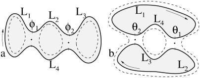
FIG. 2.: Non-trivial geometries with two tunneling points.

The coupling matrices for two-tunneling-point geometries shown in Fig. 2 are given by the expressions

$$\hat{K}^{\rm(\ref{fig:c2}a)} = \displaystyle\left|\begin{array}[c]{cc}{s_{1}s_{2}s_{4}-1\over(s_{1}-1)(s_{2}s_{4}-1)}&{s_{2}\over s_{2}s_{4}-1}\\ {s_{4}\over s_{2}s_{4}-1}&{s_{2}s_{3}s_{4}-1\over(s_{3}-1)(s_{2}s_{4}-1)}\end{array}\right|,$$ (13)

$$\hat{K}^{\rm(\ref{fig:c2}b)} = \displaystyle\left|\begin{array}[c]{cc}\textstyle{s_{1}s_{2}s_{3}s_{4}-1\over(s_{1}s_{2}-1)(s_{3}s_{4}-1)}&{s_{4}\over 1-s_{3}s_{4}}+{s_{2}\over 1-s_{1}s_{2}}\\ {s_{3}\over 1-s_{3}s_{4}}+{s_{1}\over 1-s_{1}s_{2}}&{s_{1}s_{2}s_{3}s_{4}-1\over(s_{1}s_{2}-1)(s_{3}s_{4}-1)}\end{array}\right|,$$ (16)

where $s_{i}=\exp(\omega L_{i})$. All other geometries with two tunneling points can be generated from these by replacing one or both tunneling junctions by their dual(s) as illustrated in Fig. 1b,c. Our calculation shows that the coupling matrices for thus obtained configurations are immediately related to Eqns (13), (16) as prescribed by Eq. (6): the modified coupling matrix is given by the coefficients of the Legendre-transformed bilinear form

$$\tilde{S}_{0}[\theta_{1},\phi_{2}]\!=\!{T\over 4\pi}\!\!\sum_{\omega}\omega{\bigl{(}\bar{\phi}\hat{K}\phi\!-\!\bar{\phi}_{1}\theta_{1}\!+\!\bar{\theta}_{1}\phi_{1}\bigr{)}}\bigr{|}_{K_{1\alpha}\phi_{\alpha}=\theta_{1}}.$$ (17)

This implies that under the global duality transformation, which replaces all tunneling junctions by their duals, the coupling matrix is inverted, $\tilde{K}=K^{-1}$. Combining this statement with Eq. (4), we find that the original matrix $K$ is given by the correlators of the dual fields

$$K_{\alpha\beta}={\omega\over 2\pi}\left\langle\theta_{\alpha}\bar{\theta}_{\beta}\right\rangle_{\tilde{\lambda}=0}$$ (18)

in the limit of perfect transmission (zero backscattering) in every tunneling point.

Although the dual form of the model is the result of a non-local change of variables in the path integral, the weak-coupling limits of the original model and its dual version can be interpreted as describing the same system at mutually dual filling fractions, with the total areas of the condensate and the depleted regions interchanged. This interpretation is correct as long as the probability distribution of the bare parameters of the original model, and the model at the dual filling fraction expressed in dual variables are similar, which is expected if the distribution of the disorder potential is symmetric. Under such duality “in average” $g\!\rightarrow\!g^{-1}$, and therefore at $g\neq 1$ this transformation is not an exact symmetry of the problem. This is obvious in the limit of large frequencies, where the off-diagonal elements of the coupling matrix $\hat{K}$ vanish, and the scaling dimensions of the tunneling amplitudes $\lambda_{ij}^{(k)}$ coincide with their values $\varepsilon_{k}\!=\!1\!-\!k^{2}g^{2}$ for isolated tunneling junctions.

At small frequencies, however, the interference becomes important, and the scaling behavior crosses over to mesoscopic regime where the quantization of the drift orbits is relevant. It turns out that the quadratic part of the action in this limit can be written as a simple sum

$$\lim_{\omega\rightarrow 0}\omega K_{\alpha\beta}\bar{\phi}_{\alpha}\phi_{\beta}=\sum_{\tilde{\cal C}}{1\over L_{\tilde{\cal C}}}\left|\Phi_{\tilde{\cal C}}\right|^{2},$$

where $\Phi_{\tilde{\cal C}}\equiv\sum_{\alpha\subset\tilde{\cal C}}\phi_{\alpha}$ is the directed sum of the tunneling phases $\phi_{\alpha}$ along the dual edge ${\tilde{\cal C}}$ of length $L_{\tilde{\cal C}}$ created by the global duality transformation. The presence of such terms in the action imply that variables $\Phi_{\tilde{\cal C}}$ can have only finite r.m.s. deviation, which ensures that the averages $\langle\dot{\Phi}_{\tilde{\cal C}}\rangle=\sum_{\alpha\subset{\tilde{\cal C}}}\langle\dot{\phi}_{\alpha}\rangle=0$ vanish. These constrains can be resolved by writing the phases $\phi_{\alpha}$ as the gradients $\phi_{\alpha}=g\Delta_{\alpha}{\cal V}+{\cal A}_{\alpha}$ of the local potential ${\cal V}\equiv{\cal V}_{{\cal C}}$, associated with every independent edge ${{\cal C}}$, up to some time-independent phases ${\cal A}_{\alpha}$. In this representation the model becomes identical to a disordered JJA in external magnetic field. Similarly, in the dual representation of the model the sum $\dot{\Theta}_{\cal C}=\sum_{\alpha\subset{\cal C}}\dot{\theta}_{\alpha}$ can be associated with the total current of composite bosons entering the enclosed area; this current also vanishes at zero frequency.

The performed analysis of the infrared limit reveals a deep analogy between the CB in disordered QH systems and bosons near disorder-driven superconductor–insulator (SC–I) transition. After the system is separated into weakly coupled phase-coherent areas, the terms remaining in small-frequency expansion of the action depend on lengths $L_{\alpha}$ in a highly non-universal fashion. This is used to absorb the Luttinger liquid coupling constant $g$, which renders the tunneling model independent of the filling fraction $\nu$, leading to the conclusion that all QH transitions must be in the same universality class, associated with disordered SC–I transition.

This universality follows only from the mapping between the partition functions, and it does not imply the identical transport properties. The chiral nature of the current-carrying states in the edge network model is responsible for its large Hall resistance. This can be readily seen in the integer regime using the Büttiker-Landauer[21] formula relating the four-point resistance tensor with the matrix $T_{nn^{\prime}}\!=\!|t_{nn^{\prime}}|^{2}$, $n,n^{\prime}\!=\!1,\ldots,4$ of transmission probabilities between the incoming and outgoing channels as illustrated in Fig. 1a. Although for an arbitrary unitary scattering matrix $t_{nn^{\prime}}$ the Hall resistance $R_{\rm H}=(R_{xy}-R_{yx})/2$ is not necessarily quantized, in the classical regime, which is characterized by the absence of the quantum interference between different paths contributing to $t_{nn^{\prime}}$, $R_{\rm H}=\pm 1$, in agreement with Ref.[13].

Within the proposed model, the infinite ideal leads ${\cal C}_{n}$ can be coupled with the potential gates $G_{n}$ using the action $S_{G_{n}}\!=\!2\pi\,i\,g^{-1}\!\int\!d\tau\,\Theta_{n}W_{n}$, where the phase $\Theta_{n}\!=\!\sum_{\alpha\subset{\cal C}_{n}}\theta_{\alpha}$ is proportional to the total charge transferred to the lead ${\cal C}_{n}$, and $W_{n}$ is the potential of the corresponding gate $G_{n}$. In the linear responce regime the current to the lead $n$ is given by the expression

$${\cal I}_{n}(\omega)={\omega g^{-2}}\langle\Theta_{n}\bar{\Theta}_{n^{\prime}}\rangle W_{n^{\prime}}(\omega),$$ (19)

while the equilibrium potential differences between the opposite leads can be evaluated by decomposing them into individual chiral channels, e.g.

$$2g({V}_{1}\!-\!{V}_{3})+g^{-1}({\cal I}_{2}\!-\!{\cal I}_{4})=\tilde{\cal I}_{1}\!-\!\tilde{\cal I}_{2}\!-\!\tilde{\cal I}_{3}\!+\!\tilde{\cal I}_{4}.$$ (20)

The currents

$$\tilde{\cal I}_{n}(\omega)={\omega}\langle\Phi_{n}\bar{\Theta}_{n^{\prime}}\rangle W_{n^{\prime}}(\omega),$$ (21)

are defined at the external edges $\tilde{\cal C}_{n}$ (dashed lines in Fig. 1a) in the dual representation of the model. The r.h.s. of Eq. (21) can be related to the potential difference between the phase-coherent regions of leads 1 and 3 in the effective JJA model, which leads to the formula

$$\hat{R}\!=\!-g^{-2}\hat{\Sigma}\!+\!\hat{R}_{\rm b},$$ (22)

for the resistance tensor as the sum of the quantized Hall resistance and the part $\hat{R}_{\rm b}$ associated with the transport of bosons in the JJA. An analogous decomposition $\hat{\rho}=\rho_{\rm quant}+\hat{\rho}_{\rm b}$ was previously derived[5] for resistivities in the RPA approximation; we believe this expression is exact here because the charges are essentially localized by disorder and the fluctuations of the Chern-Simons field are suppressed. The usual relationship $\hat{\rho}_{\rm b}\rightarrow\hat{\sigma}_{\rm b}^{\rm t}$ implied by the particle-vortex duality[22, 5, 9] in bulk models, is valid in the considered model only after averaging over the disorder.

Eliminating auxiliary potentials $W_{n}$ from Eqns. (19)–(21) and an expression similar to Eq. (20) for leads 2 and 4, we finally obtain

$$\hat{R}_{\rm b}\!=\!g^{2}(\hat{1}\!+\!\hat{\Sigma})\bigl{[}{\textstyle{1\over 2}}\hat{D}\,\langle\Phi\bar{\Theta}\rangle\,\langle\Theta\bar{\Theta}\rangle^{-1}\,\hat{D}^{\rm t}\bigr{]},$$ (23)

where the matrices

$$\textstyle\hat{\Sigma}=\biggl{|}\begin{array}[c]{rr}0&1\\ -1&0\end{array}\biggr{|},\quad\hat{D}=\biggl{|}\begin{array}[c]{rrrr}1&0&-1&0\\ 0&-1&0&1\end{array}\biggr{|},$$ (24)

represent the configuration of currents and potential differences in the four-lead measurement. Note that after the rescaling $g\,\Phi\rightarrow\Phi$, $\Theta/g\rightarrow\Theta$ used to construct the effective JJA model, the expression (23) loses its explicit dependence on the filling fraction $\nu=g^{2}$.

The correlator $\langle\Phi\bar{\Theta}\rangle$ in Eq. (21) is the linear combination of the expressions

$$\langle\phi_{\alpha}\bar{\theta}_{\beta}\rangle\!=\!{\textstyle{2\pi\over\omega}}\delta_{\alpha\beta}\!-\!\langle\phi_{\alpha}\bar{\phi}_{\gamma}\rangle K_{\gamma\beta}\!=\!-{\textstyle{2\pi\over\omega}}\delta_{\alpha\beta}\!+\!K_{\alpha\gamma}^{-1}\langle\theta_{\gamma}\bar{\theta}_{\beta}\rangle.$$

According to Eqns. (4) and (18), these vanish identically if the tunneling is absent in either the original ($\lambda_{\alpha}\!=\!0$) or the dual ($\tilde{\lambda}_{\alpha}\!=\!0$) representations, which leaves only the quantized part of the Hall resistance.

To conclude, we constructed the effective tunneling model which generalizes the Chalker-Coddington model[12] to the fractional QH effect. The partition function of this model can be approximately mapped to that of the disordered JJA, which implies the universality of the quantum Hall transitions. The model always has an exact dual representation, but it maps to the same system at different filling fraction only in the limit of small frequences and after averaging over disorder. The associated relationships between the filling fractions and the transport coefficients are identical to those obtained in the bulk CS model. Although in the limit of large temperatures the constructed model becomes equivalent to classical resistor network, which demonstrates[13] the QHI phenomenon, in general this behavior may not be present. Finally, since the constructed model involves no additional approximation compared with the full chiral Luttinger network model, it can be used to simulate tunneling experiments in the fractional QH regime.

It is our pleasure to acknowledge beneficial discussions with S. Chakravarty, E. Fradkin, I. Gruzberg, C. Kane, S. Kivelson, D.-H. Lee, C. Marcus, E. Shimshoni and S.-C. Zhang.

REFERENCES

- [1] R. Prange and S. M. Girvin (ed.), The Quantum Hall Effect, (Springer-Verlag, NY, 1990).
- [2] H. P. Wei, D. C. Tsui, M. A. Paalanen, and A. M. M. Pruisken, Phys. Rev. Lett. 61, 1294 (1988); L. Engel, H. P. Wei, D. C. Tsui, and M. Shayegan, Surf. Sci. 229, 13 (1990); H. P. Wei, S. W. Hwang, D. C. Tsui, and A. M. M. Pruisken, ibid. 229, 34 (1990); S. Koch, R. J. Haug, K. von Klitzing, and K. Ploog, Phys. Rev. Lett. 67, 883 (1991); L. Engel, D. Shahar, C. Kurdak, and D. Tsui, ibid. 71, 2638 (1993).
- [3] L. Wong, H. Jiang, N. Trivedi, and E. Palm, Phys. Rev. B 51, 18033 (1995).
- [4] D. Shahar et al., Phys. Rev. Lett. 74, 4511 (1995).
- [5] S. Kivelson, D.-H. Lee, and S.-C. Zhang, Phys. Rev. B 46, 2223 (1992).
- [6] S. M. Girvin and A. H. MacDonald, Phys. Rev. Lett. 58, 1252 (1987); S. C. Zhang, T. H. Hansson, and S. Kivelson, ibid. 62, 82 (1989).
- [7] D. Shahar et al., Science 274, 589 (1996).
- [8] D. Shahar et al., Sol. Stat. Commun. 102, 817 (1997).
- [9] L. Pryadko and S.-C. Zhang, Phys. Rev. B 54, 4953 (1996); E. Fradkin and S. Kivelson, Nucl. Phys. B 474, 543 (1996); L. Pryadko, Phys. Rev. B 56, 6810 (1997).
- [10] E. Shimshoni, S. L. Sondhi, and D. Shahar, Phys. Rev. B 55, 13730 (1997).
- [11] A. Dykhne and I. Ruzin, Phys. Rev. B 50, 2369 (1994); I. Ruzin and S. Feng, Phys. Rev. Lett. 74, 154 (1995).
- [12] J. Chalker and P. Coddington, J. Phys. 21, 2665 (1988).
- [13] E. Shimshoni and A. Auerbach, Phys. Rev. B 55, 9817 (1997).
- [14] A. Schmid, Phys. Rev. Lett. 51, 1506 (1983); F. Guinea, V. Hakim, and A. Muramatsu, ibid. 54, 263 (1985).
- [15] P. Fendley, A. Ludwig, and H. Saleur, Phys. Rev. B 52, 8934 (1995).
- [16] X.-G. Wen, Phys. Rev. B 41, 12838 (1990); X.-G. Wen, Int. J. Mod. Phys. B 6, 1711 (1992).
- [17] H. Yi and C. Kane, Phys. Rev. B 53, 12956 (1996).
- [18] This contribution was not taken into account in Ref.[17].
- [19] J. Jain and S. Kivelson, Phys. Rev. B 37, 4111 (1988).
- [20] Otherwise one gets unphysical selection rules for tunneling through a fractionally charged antidot [V. Pokrovsky and L. Pryadko, Phys. Rev. Lett. 72, 124 (1994).]
- [21] M. Büttiker, Phys. Rev. Lett. 57, 1761 (1986).
- [22] M. P. A. Fisher, Phys. Rev. Lett. 65, 923 (1990)