Localization length at the resistivity minima of the quantum Hall effect

Abstract

The resistivity minima of the quantum Hall effect arise due to the localization of the electron states at the Fermi energy, when it is positioned between adjacent Landau levels. In this paper we calculate the localization length $\xi$ of such states at even filling factors $\nu=2N$. The calculation is done for several models of disorder (“white-noise,” short-range, and long-range random potentials). We find that the localization length has a power-law dependence on the Landau level index, $\xi\propto N^{\alpha}$ with the exponent $\alpha$ between one and $\frac{10}{3}$, depending on the model. In particular, for a “white-noise” random potential $\xi$ roughly coincides with the classical cyclotron radius. Our results are in reasonable agreement with experimental data on low and moderate mobility samples.

I Background and results

The appearance of narrow resistivity peaks separated by deep minima is a defining feature of the quantum Hall effect (QHE). [1] The explanation of such a dependence of $\rho_{xx}$ on the magnetic field $B$ is based on the idea of localization. The states at the Fermi energy are localized at almost all $B$ except for a few discrete values $B_{N}$ where the Fermi energy is at the center of $N$th Landau level (LL). Near such special values the localization length $\xi$ is believed to diverge,

$$\xi\propto|{B-B_{N}}|^{-\gamma},$$ (1)

where $\gamma$ is a critical exponent. The analytical calculation of $\gamma$ is a notoriously difficult problem. (Numerical methods give $\gamma=2.35\pm 0.03$, see Ref. [2]). At the same time, the calculation of $\xi$ away from the critical region turns out to be much simpler. Such a calculation is the subject of the present paper. As a demonstration of the method, we calculate $\xi$ at discrete values of $B$, $B\simeq(B_{N}+B_{N+1})/2$. They correspond to the minima of $\rho_{xx}$ in the transport measurements.

Generally speaking, the definition of $\xi$ is not unique. In this paper we will adopt the following one,

$$\frac{1}{\xi}=-\lim\limits_{r\to\infty}\frac{1}{2r}\left\langle\ln|\psi(\mathchoice{{\hbox{\boldmath$\displaystyle r$}}}{{\hbox{\boldmath$\textstyle r$}}}{{\hbox{\boldmath$\scriptstyle r$}}}{{\hbox{\boldmath$\scriptscriptstyle r$}}})|^{2}\right\rangle,$$ (2)

where $\psi(\mathchoice{{\hbox{\boldmath$\displaystyle r$}}}{{\hbox{\boldmath$\textstyle r$}}}{{\hbox{\boldmath$\scriptstyle r$}}}{{\hbox{\boldmath$\scriptscriptstyle r$}}})$ is the wave function of the state at the Fermi level. The averaging is assumed to be done over the disorder realizations.

Our definition of the localization length is chosen to represent an experimentally measurable quantity. Indeed, it is well known that transport at sufficiently low temperatures proceeds via the variable-range hopping. In its turn, the hopping conduction is determined by the typical decay rate of the tails of the wave functions. Definition (2) relates $\xi$ precisely to this typical rate.

Let us further elaborate on this point. The bulk of low-temperature experimental data on the quantum Hall devices [3, 4, 5] can be successfully fit to the following dependence of $\rho_{xx}$ on the temperature $T$,

$$\rho_{xx}\propto e^{-\sqrt{T_{0}/T}},$$ (3)

which can be interpreted [6] in terms of the variable-range hopping in the presence of the Coulomb gap. [7] In this theory $T_{0}$ is directly related to $\xi$ defined by Eq. (2),

$$k_{B}T_{0}={\rm const}\,\frac{e^{2}}{\kappa\xi},$$ (4)

where $e$ is the electron charge and $\kappa$ is the dielectric constant of the medium. Using Eq. (4), one can extract the dependence of $\xi$ on $B$ from the low-$T$ transport measurements in the straightforward way. (We will discuss experimentally relevant issues in more detail in Sec. VI.)

In this paper we calculate $\xi$ using a model where the disorder is described by a Gaussian random potential $U(\mathchoice{{\hbox{\boldmath$\displaystyle r$}}}{{\hbox{\boldmath$\textstyle r$}}}{{\hbox{\boldmath$\scriptstyle r$}}}{{\hbox{\boldmath$\scriptscriptstyle r$}}})$ with the two-point correlator

$$\langle U(\mathchoice{{\hbox{\boldmath$\displaystyle r$}}}{{\hbox{\boldmath$\textstyle r$}}}{{\hbox{\boldmath$\scriptstyle r$}}}{{\hbox{\boldmath$\scriptscriptstyle r$}}}_{1})U(\mathchoice{{\hbox{\boldmath$\displaystyle r$}}}{{\hbox{\boldmath$\textstyle r$}}}{{\hbox{\boldmath$\scriptstyle r$}}}{{\hbox{\boldmath$\scriptscriptstyle r$}}}_{2})\rangle=C(|\mathchoice{{\hbox{\boldmath$\displaystyle r$}}}{{\hbox{\boldmath$\textstyle r$}}}{{\hbox{\boldmath$\scriptstyle r$}}}{{\hbox{\boldmath$\scriptscriptstyle r$}}}_{1}-\mathchoice{{\hbox{\boldmath$\displaystyle r$}}}{{\hbox{\boldmath$\textstyle r$}}}{{\hbox{\boldmath$\scriptstyle r$}}}{{\hbox{\boldmath$\scriptscriptstyle r$}}}_{2}|).$$ (5)

We will assume that function $C(r)$ becomes small at $r$ larger than some distance $d$ and that $C(r)$ does not have any other characteristic lengths. The rms amplitude of the potential, $\sqrt{C(0)}$, will be denoted by $W$. We will assume that $W$ is much smaller than $E_{F}$, the Fermi energy. The electron-electron interaction is ignored at this stage.

To facilitate the presentation of our results we would like to introduce the phase diagram shown in Fig. 1. The vertical axis stands for the dimensionless parameter $k_{F}d$, where $k_{F}$ is the Fermi wave-vector of the two-dimensional electron gas, $k_{F}=\sqrt{2\pi n}$, $n$ being the electron gas density. The horizontal axis is the LL index $N\simeq(k_{F}l)^{2}/2$, where $l=\sqrt{\hbar c/eB}$ is the magnetic length. The Fermi level is assumed to be at the midpoint between the centers of $N$th and $N+1$st LLs. The axes are in the logarithmic scale. The ratio $W/E_{F}$ is assumed to be fixed.

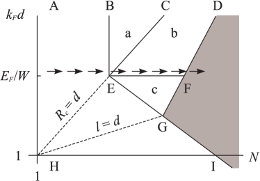
FIG. 1.: The parameter space of the problem with a monoscale random potential [Eqs. (5) and (15)]. The entire phase space is divided into regions with different dependence of $\xi$ on $N$ and $k_{F}d$. The boot-shaped region AHIGEB is described by Eq. (16), the shaded region to the right of the line DFGI by Eqs. (8) and (9), the region BEGFD by Eq. (1), and finally, the region below the line HI by Eq. (1). The arrows show the “trajectory,” traced by a “standard” sample (see definition in Sec. VI) as the magnetic field decreases.

Several lines drawn in Fig. 1 divide the phase plane into the regions with different dependence of $\xi$ on $B$. Let us explain the physical meaning of these lines. The line BEGI is the line where the densities of states of neighboring LLs start to overlap as $N$ increases ($B$ decreases). Thus, to the right of this line the density of states at the Fermi level is practically equal to its zero field value. We will refer to this region of the parameter space as the region of overlapping LLs. To the left of the line BEGI only the tails of the neighboring LLs reach the Fermi level and the density of states is much smaller than at zero field. This region will be called the region of discrete LLs. The equation, of the line EGI is (cf. Refs. [8, 9, 10])

$${\rm EGI}:\>k_{F}d\sim\frac{1}{N}\left(\frac{E_{F}}{W}\right)^{2}.$$ (6)

Another line in Fig. 1, GFD, separates the regions of different dynamic properties. To the left of this line the guiding centers of the cyclotron orbits would perform the regular drift along certain closed contours. This phenomenon has been dubbed “classical localization” in Ref. [11]. To the right of the line GFD (shaded sector in Fig. 1) the motion of the guiding center is diffusive (on not too large length scales). The equation for the line GFD has been derived in Ref. [11],

$${\rm GFD}:\>k_{F}d\sim N\left(\frac{W}{E_{F}}\right)^{2/3}.$$ (7)

In the diffusive region the calculation of $\xi$ reduces to the calculation of the “classical” conductivity $\sigma_{xx}$ by means of the ansatz (for discussion and bibliograthy see Refs.[2] and [11])

$$\xi\propto\exp\left[\pi^{2}\left(\frac{h}{e^{2}}\sigma_{xx}\right)^{2}\right],\quad\sigma_{xx}\gg\frac{e^{2}}{h}.$$ (8)

The “classical” $\sigma_{xx}$ is to be calculated by virtue of the Einstein relation, i.e., as a product of quantum density of states and the classical diffusion coefficient. The physical mechanism of the localization in this region is the destructive interference of the classical diffusion paths. The calculation of the “classical” $\sigma_{xx}$ to the right of the line GFD and in the logarithmically narrow sector to its left (where $\sigma_{xx}$ is still larger than $\frac{e^{2}}{h}$) has been done in Ref. [11] in some detail. As one can see from Eqs. (6) and (7), the studied region corresponds to rather long range of the random potential, $k_{F}d>(E_{F}/W)^{2/3}$. However, Eq. (8) applies for smaller values of parameter $k_{F}d$ as well. That is as long as we stay to the right of the line GI. In the entire shaded sector to the right of DFGI the motion is diffusive. The corresponding “classical” $\sigma_{xx}$ is given by the usual Drude-Lorentz formula

$$\sigma_{xx}=\frac{\sigma_{0}}{1+(\omega_{c}\tau)^{2}}.$$ (9)

Equations (8) and (9) enable one to calculate $\xi$ up to a pre-exponential factor. In this sector $\xi$ is exponentially large.

As $N$ decreases and the boundary DFGI of the diffusive region is crossed, the “classical” $\sigma_{xx}$ rapidly falls off. Above the point G this is brought about by the aforementioned “classical localization”; below the point G it is caused by the rapid decrease of the density of states at the Fermi level. Already slightly to the left of the line DFGI the “classical” $\sigma_{xx}$ becomes much less than $\frac{e^{2}}{h}$ and the ansatz (8) loses its domain of applicability. On the physical level, the nature of the particle motion changes: the diffusion is replaced by quantum tunneling. This paper is devoted to the calculation of $\xi$ in the tunneling regime (unshaded area in Fig. 1).

One has to discriminate between the tunneling in the case of overlapping LLs and in the case of discrete LLs. The former is realized in the region above the line BEGFD. The idea of the derivation of $\xi$ in this regime belongs to Mil’nikov and Sokolov [12] who applied it to the lowest Landau level. [13] The argument goes as follows. In the described regime the density of states near the Fermi level is high. On the quasiclassical level such states can be thought of as a collection of close yet disconnected equipotential contours, along which the particle can drift according to the classical equations of motion. Nonzero $\xi$ appears as a result of the quantum tunneling through the classically forbidden areas between adjacent contours. The localization length is determined by the spatial extent of relevant equipotential contours and by the characteristic tunneling amplitude.

Reference [12] has been criticized in literature for, e.g., neglecting the interference effects. In our opinion this criticism is unjustified. The authors of Ref. [12] have clearly indicated the domain of applicability of their theory. It can be verified that within this domain the amplitude of tunneling between the pairs of contours is small; hence, the probability of return to the initial point after at least one tunneling event is also small. In this case the interference phenomena can be safely ignored (cf. Ref. [2]).

The case of high Landau levels requires some modifications to the original method of Mil’nikov and Sokolov. The details are given in Sec. V. We have found that the region of the phase space bounded by the line BEGFD consists, in fact, of three smaller regions (see Fig. 1) with different dependence of $\xi$ on $N$:

$$\displaystyle k_{F}\xi \sim \frac{N^{10/3}}{k_{F}d}\left(\frac{W}{E_{F}}\right)^{7/3}$$ (11)

$$\sim \frac{N^{5/2}}{(k_{F}d)^{1/6}}\left(\frac{W}{E_{F}}\right)^{7/3}$$ (12)

$$\sim N^{5/2}(k_{F}d)^{1/2}\left(\frac{W}{E_{F}}\right)^{3}$$ (13)

(the equation labels match the region labels in Fig. 1). The boundary EC, which separates the regions I and II, is given by

$${\rm EC}:\>k_{F}d\sim N.$$ (14)

The variety of different subregimes in the region BEGFD appears because of an interplay among three important length scales of the problem: the correlation length $d$ of the random potential, the cyclotron radius $R_{c}=(2N+1)/k_{F}$, and the percolation length $\xi_{\rm perc}$ (the typical diameter of the relevant equipotential contours). In this connection note that Eq. (14) is simply $R_{c}\sim d$.

Compared to such a variety, the situation in the region of discrete LLs (AHIGEB) is very simple: the dependence of $\xi$ on $N$ is given by a single formula. Suppose that the Fourier transform $\tilde{C}(q)$ of the correlator $C(r)$ [see Eq.(5)] has the form

$$\tilde{C}(q)=\tilde{C}(0)\,\exp\!\left[-\frac{1}{\beta}(qd)^{\beta}\right],\quad\beta>1,$$ (15)

then $\xi$ is given by

$$\xi\simeq\left(\frac{2\beta}{\beta-1}\ln\frac{\hbar\omega_{c}}{W}\right)^{-\frac{\beta-1}{\beta}}\frac{2l^{2}}{d}.$$ (16)

The logarithmic factor neglected, this can be written as

$$\xi\sim\frac{R_{c}}{k_{F}d}.$$ (17)

Formula (16) has previously appeared (for $\beta=2$) in the work of Raikh and Shahbazyan. [14] These authors considered the case of the lowest LL ($N=0$) but suggested that it is also valid for $R_{c}\ll d$, i.e., within the knife-shaped region AHEB. We demonstrate that Eq. (16) is in fact valid in a much larger domain. The differences between this work and Ref. [14] are outlined in the end of Sec. IV.

The only part of the phase diagram we have not discussed yet is the area of “white-noise” potential. It is located below the line HI, i.e., $k_{F}d=1$. The corresponding formula for $\xi$ is

$$\displaystyle\xi = \frac{2R_{c}}{\cal L},\quad{\cal L}\ll 2N+1,$$ (19)

$$= \frac{l}{\sqrt{\cal L}},\quad{\cal L}\gg 2N+1,$$ (20)

$$\displaystyle{\cal L} \simeq \ln\left(\frac{\hbar\omega_{c}l}{Wd}\right),$$ (21)

which matches Eq. (16) at $k_{F}d\sim 1$. Previously, formula (20) has been obtained by Shklovskii and Efros [15] and also by Li and Thouless [16] for the lowest LL, $N=0$.

Neglecting the logarithmic factor, we can write Eq. (19) in a remarkably simple form,

$$\xi\sim R_{c}.$$ (22)

Remarkably, the quantum localization length $\xi$ is determined by a purely classical quantity, the cyclotron radius!

The basic idea used in the derivation of Eqs. (16) and (1) is to study not the tunneling of the particle itself but the tunneling of the guiding center $\textstyle\rho$ of its cyclotron orbit. For definiteness, consider the tunneling in the $y$-direction. The effect of the magnetic field can be modelled by means of the effective “magnetic” potential,

$$U_{m}(y)=\frac{m\omega_{c}^{2}(y-\rho_{y})^{2}}{2},$$ (23)

acting on the particle. The classical turning points for this type of potential are at the distance $R_{c}$ from $\rho_{y}$. Therefore, if $\rho_{y}$ does not change its position, the longest distance that the particle can travel without getting under the magnetic barrier is $2R_{c}$. And since the barrier increases with $y$, the suppression of the wave function, which starts beyond this distance, is faster than a simple exponential.

In the absence of the random potential, $\rho_{y}$ is a good quantum number; however, if the external potential is present, it can scatter the particle, which would cause a change in the guiding center position. Such a “scattering-assisted” tunneling modifies the overall decay of the wave function [17, 15, 16] from the super-exponential to the plain exponential one,

$\displaystyle\psi(0,y)\sim e^{-y/\xi}.$

Denote a typical displacement of the guiding center after one scattering act by $\Delta\rho_{y}$. The physical picture of tunneling depends on the relation between $\Delta\rho_{y}$ and $2R_{c}$.

The case $\Delta\rho_{y}>2R_{c}$, which is typically realized at the lowest LL, has been studied previously in Refs. [15, 16, 17]. In this case the tunneling involves the propagation under the magnetic barrier. Note that the barrier itself no longer increases as $y$ squared, which would be with $\rho_{y}={\rm const}$ [see Eq. (23)]. After a series of displacements of the guiding center, the barrier acquires a saw-tooth shape. In this regime the under-barrier suppression is an important factor in the overall decay of the wave function.

In contrast to the lowest LL, at high LLs ($N\gg 1$) where $R_{c}$ is large, the inequality of the opposite sense, i.e., $\Delta\rho_{y}\leq 2R_{c}$, is typically realized. In this case the particle does not propagate under the magnetic barrier at all! However, the tunneling a distance $y\gg\Delta\rho_{y}$ requires a large number $M\sim y/\Delta\rho_{y}$ of the scattering acts. The amplitude of each act is proportional to $W$ and is inversely proportional to a large energy denominator $E=E_{F}-\hbar\omega_{c}(N+\frac{1}{2})$. At the resistivity minima of the QHE, which we are mainly interested in, $E=\hbar\omega_{c}/2\gg W$ (discrete LLs), which implies that the typical scattering amplitude is small and that the wave function decays exponentially with $y$ even though the electron never propagates under the magnetic barrier (this argument is simply a verbal representation of the locator expansion).

The case of the “white noise” potential is quite illuminating in this respect. The optimal tunneling path is sketched in Fig. 2. The optimization is based roughly on the requirement that each scattering event should displace the guiding center by the largest possible distance without placing the particle under the magnetic barrier. Clearly, this distance is equal to $2R_{c}$, which makes the tunneling trajectory look like a classical skipping orbit near a hard wall, see Fig. 2.

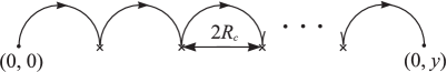
FIG. 2.: The optimal tunneling trajectory of an electron in the random potential of the “white-noise” type. Crosses symbolize the scattering acts. The direction of the $y$-axis is from the left to the right.

Let us estimate the localization length corresponding to this optimal path. Since $\Delta\rho_{y}\simeq 2R_{c}$, the number of the scattering events needed to travel the distance $y$ is $M\simeq y/(2R_{c})$. As discussed above, after each event the wave function decreases by a factor of the order of $W/(\hbar\omega_{c})$. Hence, the overall suppression factor is $(\hbar\omega_{c}/W)^{-M}$, which means that $\xi\sim 2R_{c}/\ln(\hbar\omega_{c}/W)$ in agreement with Eq. (19). This derivation will be done more carefully in Sec. III.

Formula (16) can be derived in a similar way. After each scattering event the wave function decreases by a factor of the order of $f=(W/E)\exp[-(1/2\beta)(qd)^{\beta}]$ where $q=\Delta\rho_{y}/l^{2}$ is the typical wave vector absorbed in the scattering act. The total suppression factor after propagating the distance $y$ is of the order of $f$ to the power $y/\Delta\rho_{y}$. Optimizing this suppression factor with respect to $\Delta\rho_{y}$, one arrives at Eq. (16). A detailed derivation will be done in Sec. III.

The paper is organized as follows. Section II is devoted to general considerations and qualitative derivation of Eq. (16) and (1). In Sec. III this derivation is made more rigorous assuming that the random potential is short-range (or “white-noise”). In Sec. IV we consider the long-range potential in the regime of discrete LLs. The approach is different from that of Sec. III but the final result, Eq. (16), is the same as for the short-range case. In Sec. V we consider the case of overlapping LLs. The variety of regimes in Eq. (1) is explained with the help of results developed in the field of statistical topography. [18] Finally, in Sec. VI we compare our results with available experimental data for moderate mobility samples and propose a method to perform the measurements with modern high-mobility devices.

II General considerations

Following the overwhelming majority of papers in the field, we will take advantage of the single Landau level approximation. In this approximation the original Hilbert space is truncated to the functions, which belong to the particular ($N$th) Landau level. It is conventional to choose the orthonormal set of functions

$$\displaystyle\psi_{n}(x,y) = \frac{e^{\frac{i}{\hbar}\rho_{n}x}}{\sqrt{L_{x}}}\Phi_{N}(y+\rho_{n}),$$ (24)

$$\displaystyle\Phi_{N}(y) = \frac{1}{\sqrt{2^{N}n!\,l\pi^{1/2}}}e^{-y^{2}/2l^{2}}H_{N}\left(\frac{y}{l}\right),$$ (25)

$$\rho_{n} = \frac{2\pi l^{2}}{L_{x}}n,\quad n=0,1,\ldots$$ (26)

to be our basis states. Here $L_{x}$ is the $x$-dimension of the system and $H_{N}(z)$ is the Hermite polynomial. Such functions are the eigenfunctions of the Hamiltonian

$$H=\frac{(\mathchoice{{\hbox{\boldmath$\displaystyle p$}}}{{\hbox{\boldmath$\textstyle p$}}}{{\hbox{\boldmath$\scriptstyle p$}}}{{\hbox{\boldmath$\scriptscriptstyle p$}}}+\frac{|e|}{c}\mathchoice{{\hbox{\boldmath$\displaystyle A$}}}{{\hbox{\boldmath$\textstyle A$}}}{{\hbox{\boldmath$\scriptstyle A$}}}{{\hbox{\boldmath$\scriptscriptstyle A$}}})^{2}}{2m}+U(\mathchoice{{\hbox{\boldmath$\displaystyle r$}}}{{\hbox{\boldmath$\textstyle r$}}}{{\hbox{\boldmath$\scriptstyle r$}}}{{\hbox{\boldmath$\scriptscriptstyle r$}}})$$ (27)

in the Landau gauge, $\mathchoice{{\hbox{\boldmath$\displaystyle A$}}}{{\hbox{\boldmath$\textstyle A$}}}{{\hbox{\boldmath$\scriptstyle A$}}}{{\hbox{\boldmath$\scriptscriptstyle A$}}}=(By,0,0)$, provided there is no external potential ($U\equiv 0$).

The single Landau level approximation works well if the cyclotron frequency $\omega_{c}$ is the fastest frequency in the problem. This is obviously the case for the discrete LLs, i.e., in the region AHIGEB in Fig. 1. It is less trivial and it was demonstrated in Ref. [11] that the inter-LL transitions are suppressed in the region above the line BEGFD as well. When such transitions are neglected, the guiding center coordinates, $\rho_{y}=y-(v_{x}/\omega_{c})$ and $\rho_{x}=x+(v_{y}/\omega_{c})$ become the only dynamical variables in the problem.

Since the random potential is assumed to be isotropic, so is the ensemble averaged decay of the wave functions. With the above choice of the basis, however, it is convenient to study such a decay in the $y$-direction: from the point $(0,0)$ to the point $(0,y)$.

As the next step we notice that the guiding center coordinates satisfy the commutation relation

$\displaystyle\left[\rho_{y},\rho_{x}\right]=il^{2}.$

Thus, $\rho_{y}$ plays the role of the canonical coordinate while the quantity $(\hbar/l^{2})\rho_{x}$ is the canonical momentum. It is therefore natural to use the $\rho_{y}$-representation for the wave functions. For example, in this representation wave functions (24) become delta-functions. In general, the transformation rule between the two representations, $\psi(x,y)$ and $\phi(\rho_{y})$, is given by the formula,

$$\psi(x,y)=\int\frac{d\rho_{y}}{\sqrt{2\pi l^{2}}}\,\Phi_{N}(y-\rho_{y})\,\phi(\rho_{y})\,e^{-\frac{i}{l^{2}}x\rho_{y}}.$$ (28)

Definition (2) of the localization length can also be written in terms of the electron’s Green’s function $G$,

$$\frac{1}{\xi}=-\lim\limits_{y\to\infty}\frac{1}{y}\left\langle\ln|G(0,y;E)|\right\rangle.$$ (29)

On the other hand, Eq. (28) leads to the following Green’s function transformation rule for $G(0,y;E)$,

$$G=\int\!\frac{d\rho_{1}d\rho_{2}}{2\pi l^{2}}\,\Phi_{N}(\rho_{1})\,\Phi_{N}(\rho_{2})\,G_{\rho}(\rho_{1},\rho_{2}+y;E),$$ (30)

where $G_{\rho}(\rho_{1},\rho_{2};E)$ is the Green’s function in the guiding center representation (as in Sec. I the energy $E$ is referenced to the Landau level center, and so we are interested mostly in the case $|E|=\hbar\omega_{c}/2$).

Green’s function $G_{\rho}(\rho_{1},\rho_{2};E)$ satisfies the Schröedinger equation (with the delta-function as a source)

                                                                                 

$$G_{\rho}(\rho_{1},\rho_{2};E)=\frac{\delta(\rho_{1}-\rho_{2})}{E}+\frac{1}{L_{x}}\sum_{q_{x}}U_{0}(\tilde{q}_{x},\rho_{1}+\frac{1}{2}q_{x}l^{2})\,G_{\rho}(\rho_{1}+q_{x}l^{2},\rho_{2};E),$$ (31)

                                                                               

where the tilde indicates the Fourier transform over the corresponding argument. The quantity $U_{0}$ has the meaning of the random potential averaged over the cyclotron orbit (cf. Refs. [9, 11]),

$$\tilde{U}_{0}(\mathchoice{{\hbox{\boldmath$\displaystyle q$}}}{{\hbox{\boldmath$\textstyle q$}}}{{\hbox{\boldmath$\scriptstyle q$}}}{{\hbox{\boldmath$\scriptscriptstyle q$}}}) = \tilde{U}(\mathchoice{{\hbox{\boldmath$\displaystyle q$}}}{{\hbox{\boldmath$\textstyle q$}}}{{\hbox{\boldmath$\scriptstyle q$}}}{{\hbox{\boldmath$\scriptscriptstyle q$}}})\,F_{N}(ql^{2}),$$ (32)

$$\displaystyle F_{N}(y) = L_{N}\left(\frac{y^{2}}{2l^{2}}\right)\,e^{-y^{2}/4l^{2}},$$ (33)

$L_{N}(z)$ being the Laguerre polynomial (the tilde over the symbol itself indicates the two-dimensional Fourier transform).

As discussed in the previous section, in the absence of the random potential, $\rho_{y}$ is a good quantum number. The tunneling requires propagation under the magnetic barrier, which leads to a super-exponential decay of $G(0,y;E)$. Indeed, in the absence of the random potential $G_{\rho}(\rho_{1},\rho_{2};E)=\delta(\rho_{1}-\rho_{2})/E$ [see Eq. (31)]. Upon substitution into Eq. (30) one recovers the well-known expression for the Green’s function in the clean case,

$$G(0,y;E)=\frac{F_{N}\left(y\right)}{2\pi l^{2}E}.$$ (34)

Since $F_{N}(y)$ is the product of a polynomial and a Gaussian [see Eq. (33)], the Green’s function $G(0,y;E)$ decays faster than the exponential at large $y$. In view of definition (29) this means that $\xi=0$. In fact, the structure of Eq. (30) suggests that nonzero $\xi$, i.e., a simple exponential decay of $G$, is possible only if $G_{\rho}$ decays no faster than a simple exponential. In other words, $\xi$ is nonzero only if $\xi_{\rho}$ is nonzero where

$$\frac{1}{\xi_{\rho}}=-\lim\limits_{\rho\to\infty}\frac{1}{\rho}\left\langle\ln|G_{\rho}(0,\rho;E)|\right\rangle$$ (35)

[compare with the definition of $\xi$, Eq. (29)]. Unfortunately, $\xi$ and $\xi_{\rho}$ may differ. Only the inequality

$$\xi_{\rho}\geq\xi$$ (36)

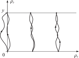
FIG. 3.: Tunneling paths of the guiding center (schematically). Green’s function $G(0,y;E)$ is a sum over the paths near $\rho_{x}=0$; Green’s function $G_{\rho}(0,y;E)$ is a sum over all the possible paths connecting the lines $\rho_{y}=0$ and $\rho_{y}=y$.

is guaranteed to be met. Indeed, $G_{\rho}(\rho_{1},\rho_{2};E)$ typically behaves like $G_{\rho}\sim e^{-|\rho_{2}-\rho_{1}|/\xi_{\rho}+i\phi(\rho_{1},\rho_{2})}$. If the phase $\phi(\rho_{1},\rho_{2})$ is a smooth function of coordinates, then $|G(0,y;E)|\sim|G_{\rho}(0,y;E)|$, and $\xi=\xi_{\rho}$. Otherwise, the integrand in Eq. (30) oscillates rapidly, $|G(0,y;E)|\ll|G_{\rho}(0,y;E)|$ and $\xi<\xi_{\rho}$. On a physical level, $\xi$ describes the tunneling between two point-like contacts while $\xi_{\rho}$ characterizes the tunneling between two infinite parallel leads. While the Feynman paths contributing to the former process make up a narrow bundle near $\rho_{x}=0$ (Fig. 3), the latter one gathers contributions of many such bundles. As a result, the amplitude of the latter process is much larger on the account of rare places (“pinholes”) where the tunneling is unusually strong.

Nevertheless, in many cases $\xi$ and $\xi_{\rho}$ are very close to each other; for instance, when the random potential is short-range (see the next section).

Next we would like to present a simple yet very instructive model. This model has a great advantage of being solvable.

Suppose that the averaged random potential has the form

$$U_{0}(\mathchoice{{\hbox{\boldmath$\displaystyle\rho$}}}{{\hbox{\boldmath$\textstyle\rho$}}}{{\hbox{\boldmath$\scriptstyle\rho$}}}{{\hbox{\boldmath$\scriptscriptstyle\rho$}}})=U_{1}(\rho_{y})+e^{i\rho_{x}q}U_{2}(\rho_{y})+e^{-i\rho_{x}q}\,U_{2}^{\ast}(\rho_{y}),$$ (37)

where $U_{1}$, ${\rm Re}\,U_{2}$, and ${\rm Im}\,U_{2}$ are mutually independent Gaussian random variables. Similar to the above, we will assume that they have amplitude $W$ and correlation length $d$. A simpler model with $\rho_{y}$-independent $U_{1}$, ${\rm Re}\,U_{2}$, and ${\rm Im}\,U_{2}$ has been studied in Refs. [14] and [19].

For the model potential (37) all the points along the $\rho_{x}$ axis are statistically equivalent; the “pinholes” we mentioned above are absent; therefore, $\xi=\xi_{\rho}$.

From Eq. (31), we see that the matrix element $\langle\rho_{1}|U_{0}|\rho_{2}\rangle$ is zero unless $\rho_{1}=\rho_{2}$ or $\rho_{1}-\rho_{2}=\pm ql^{2}$. It is convenient to assume that $ql^{2}$ is divisible into $2\pi l^{2}/L_{x}$, the smallest distance between the centers of gravity of the basis states (24). In other words, we will assume that $L_{x}q/(2\pi)$ is an integer. Under this condition, the system can be split into $L_{x}q/(2\pi)$ independent chains (Fig. 4). The guiding center coordinates $\{\rho_{n}\}$ in each chain form an equidistant set: $\rho_{n+1}-\rho_{n}=ql^{2}$. The hopping is allowed only between the nearest neighbors of the same chain and is characterized by the hopping amplitude $U_{2}^{\ast}[(\rho_{n}+\rho_{n+1})/2]$. As for $U_{1}(\rho_{n})$, it plays the role of the on-site energy.

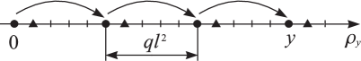
FIG. 4.: The model system. Each vertical tick corresponds to one of the basis states $\psi_{n}$. The distance between the ticks is $2\pi l^{2}/L_{x}$. The hopping (symbolized by arrows) is possible at (much larger) distance $ql^{2}$, and takes place between the states forming an equidistant chain. Two of such chains (one marked by the dots and the other by the triangles) are shown.

The localization length of a disordered chain is given by the exact formula due to Thouless, [20] which in our case reads

$$\frac{ql^{2}}{\xi}=\int\!dE^{\prime}D(E^{\prime})\ln|E-E^{\prime}|-\left\langle\ln|U_{2}(\rho)|\right\rangle,$$ (38)

$D(E)$ being the disorder-averaged density of states normalized by the condition $\int\!dE\,D(E)=1$. It is noteworthy that $D(E)$ can in principle be found exactly if all the matrix elements are statistically independent, [21] i.e., if $ql^{2}\gg d$. If this is not the case, then $D(E)$ can be calculated by some approximation scheme. At any rate, $D(E)$ is small if $|E|\gg W$ (see e.g., Lifshitz et al. [22]). In this case we can expand the logarithm in Eq. (38) in the powers of $E^{\prime}/E$ to obtain

$$\frac{1}{\xi}=\frac{1}{ql^{2}}\left[\left\langle\!\ln\left|\frac{E}{U_{2}}\right|\,\right\rangle+O\left(\frac{W}{E}\right)^{2}\right].$$ (39)

Taking the average in Eq. (39), we obtain

$$\frac{1}{\xi}=\frac{1}{ql^{2}}\left[\ln\left|\frac{E}{W}\right|-\frac{\ln 2-{\bf C}}{2}+O\left(\frac{W}{E}\right)^{2}\right],$$ (40)

where ${\bf C}=0.577\ldots$ is the Euler constant.

It is quite remarkable that $\xi$ does not depend on whether the successive hopping terms $U_{2}^{\ast}[(\rho_{n}+\rho_{n+1})/2]$ are correlated or not. With the high degree of accuracy, $O(W^{2}/E^{2})$, the localization length has the same value for $ql^{2}>d$ (“short-range” disorder) and $ql^{2}<d$ (“long-range” disorder).

The qualitative derivation of Eq. (40) can be done with the help of the locator expansion (see a similar argument in the preceding section). The tunneling through a distance $y$ is achieved by a minimum of $M=y/(ql^{2})$ hops. Each hop is characterized by the hopping amplitude of the order of $W/E$. Thus, the suppression factor of the wave function over a distance $y$ is of the order of $(W/E)^{M}$. On the other hand, this factor is equal to $e^{-y/\xi}$, which leads to Eq. (40).

Let us now return to the original problem with the two-demensional random potential [Eqs. (5) and (15)]. Leaving a more rigorous calculation for the next two sections, we will present heuristic arguments leading to Eqs. (16) and (1).

Let us divide the entire spectrum of Fourier harmonics of the random potential $U_{0}$ into bands $q_{n}-\frac{1}{2}\Delta q<q_{x}<q_{n}+\frac{1}{2}\Delta q$, $n=1,2,\ldots$ of width $\Delta q\sim 1/d$. Denote by $U_{q}(\mathchoice{{\hbox{\boldmath$\displaystyle\rho$}}}{{\hbox{\boldmath$\textstyle\rho$}}}{{\hbox{\boldmath$\scriptstyle\rho$}}}{{\hbox{\boldmath$\scriptscriptstyle\rho$}}})$ the combined amplitude of the harmonics, which make up the band centered at $q$,

$$U_{q}(\mathchoice{{\hbox{\boldmath$\displaystyle\rho$}}}{{\hbox{\boldmath$\textstyle\rho$}}}{{\hbox{\boldmath$\scriptstyle\rho$}}}{{\hbox{\boldmath$\scriptscriptstyle\rho$}}})=\int\limits_{q-\frac{1}{2}\Delta q}^{q+\frac{1}{2}\Delta q}\!\!\frac{dq_{x}}{2\pi}\,{U}_{0}(\tilde{q}_{x},\rho_{y})\,e^{i\rho_{x}q_{x}},$$ (41)

If $q\gg 1/d$, the corresponding band is very narrow, and $U_{q}$ as a function of $\rho_{x}$ looks very much like a plain wave, $U_{q}\propto e^{iq\rho_{x}}$, exactly as $U_{2}$ in the model problem. Suppose that the scattering caused by different bands can be considered independently. In this case each band generates its own decay rate $1/\xi(q)$ of the wave function. By analogy with Eq. (39), we can write

$$\frac{1}{\xi(q)}\simeq\frac{1}{2ql^{2}}\left\langle\!\ln\left|\frac{E^{2}}{W_{q}^{2}}\right|\,\right\rangle,$$ (42)

where $W_{q}^{2}$ is the variance of $U_{q}(\mathchoice{{\hbox{\boldmath$\displaystyle\rho$}}}{{\hbox{\boldmath$\textstyle\rho$}}}{{\hbox{\boldmath$\scriptstyle\rho$}}}{{\hbox{\boldmath$\scriptscriptstyle\rho$}}})$,

$$W_{q}^{2}\sim C_{0}(\tilde{q},0)\,\Delta q,$$ (43)

and $\tilde{C}_{0}(q)$ is the correlator of the averaged potential,

$$\tilde{C}_{0}(q)=\tilde{C}(q)\left[F_{N}(ql^{2})\right]^{2}.$$ (44)

Let $q_{\ast}$ be the wave vector corresponding to the largest $\xi(q)$, then it is natural to think that $\xi=\xi(q_{\ast})$. In other words, the localization length should be determined by the “optimal band” of harmonics, which we are going to find next.

In view of Eq. (44), two cases have to be distinguished, $q_{\ast}<2k_{F}$ and $q_{\ast}>2k_{F}$. The latter is realized for a sufficiently weak “white-noise” random potential, the former for the potentials of all other types.

If $q<2k_{F}$, then $C_{0}(\tilde{q},0)$ differs from $C(\tilde{q},0)$ only by a pre-exponential factor. Using Eqs. (15) and (43) and omitting some unimportant pre-exponential factors, we arrive at

$$\frac{1}{\xi(q)}\simeq\frac{1}{ql^{2}}\left[\ln\left|\frac{E}{W}\right|+\frac{(qd)^{\beta}}{2\beta}\right].$$ (45)

If $\beta>1$, then $\xi(q)$ given by Eq. (45) has the maximum at

$$q_{\ast}(E)=\frac{1}{d}\left(\frac{2\beta}{\beta-1}\ln\left|\frac{E}{W}\right|\right)^{\frac{1}{\beta}}.$$ (46)

Substituting this value into Eq. (45) and taking $E=\hbar\omega_{c}/2$, we obtain Eq. (16).

The qualitative derivation of Eq. (1) goes along the same lines. The sole difference is that $q_{\ast}$ turns out to be close or even larger that $2k_{F}$ and at the same time smaller than $1/d$. In this case $\tilde{C}_{0}(q_{\ast})$ is determined by $F_{N}(q_{\ast}l^{2})$ rather than by $\tilde{C}(q_{\ast})$. (In this case, of course, the appropriate width $\Delta q$ of the bands is much smaller than $1/d$, but the basic idea of dividing the spectrum into independent bands stays).

III Short-range random potential

In this section we present a more detailed calculation of the localization length for the short-range random potential, $d\ll l$. As we mentioned in the preceding section, Thouless formula (39) is in agreement with the locator expansion for $G_{\rho}$,

$$G_{\rho}(0,Mql^{2};E)\simeq\frac{L_{x}}{2\pi l^{2}E}\prod_{m=1}^{M}\frac{U_{2}^{\ast}\left[\left(m-\frac{1}{2}\right)ql^{2}\right]}{E}.$$ (47)

The equivalent of Eq. (47) in the general case is

$$\displaystyle G_{\rho}(0,y;E)\simeq\frac{1}{E}\sum_{M=0}^{\infty}\int\frac{dq_{1}}{2\pi}\int\frac{dq_{2}}{2\pi}\ldots\int\frac{dq_{M}}{2\pi}$$ (48)

$$\displaystyle\times\delta\left(y-l^{2}\sum_{n=1}^{M}q_{n}\right)\prod_{m=1}^{M}\frac{U_{0}^{\ast}\left(\tilde{q}_{m},\rho_{my}\right)}{E},$$ (49)

where $\rho_{my}$ stands for

$$\rho_{my}=l^{2}(q_{1}+q_{2}+\ldots+q_{m-1}+\frac{1}{2}q_{m}).$$ (50)

Combining Eqs. (30) and (49), we arrive at

$$G^{(M)}(0,y;E)=\sum_{M=0}^{\infty}G^{(M)},$$ (51)

$$G^{(M)}\simeq\int\frac{d\rho}{2\pi l^{2}E}\,\Phi_{N}(\rho)\,\Phi_{N}(\rho+\Sigma-y)$$ (52)

$$\times\int\ldots\int\!\prod_{m=1}^{M}\frac{dq_{m}}{2\pi E}\,U_{0}^{\ast}\left(\tilde{q}_{m},\rho+\rho_{my}\right),$$ (53)

where $\Sigma=\sum_{n=1}^{M}q_{n}l^{2}$.

Formula (49) is certainly just an approximation. However, the model studied in the preceding section showed that the the relative error in calculating $\xi$ in this way is of the order $O\left(W/E\right)^{2}$, which is quite satisfactory. The major defect of our approximation is having all the energy denominators equal to $E$. Consequently, this approximation scheme does not capture the phenomenon of the resonant tunneling, [22] which appears due to anomalously small energy denominators. Note however that our goal is to calculate $\langle\ln|G(0,y;E)|\rangle$. The resonant tunneling configurations are exponentially rare and do not contribute to this quantity. In the model studied in the previous section this can be seen explicitly: the resonant tunneling configurations correspond to $E=E^{\prime}$ in Eq. (38) where the integrand diverges. However, the divergence is integrable, and moreover has an exponentially small weight.

We calculate $\langle\ln|G(0,y;E)|\rangle$ in three steps. First, we calculate $\langle|G(0,y;E)|^{2}\rangle_{\rm nr}$, where the subscript “nr” stands for “non-resonant,” i.e., with resonant tunneling configurations excluded. The reminder of such an exclusion is essential in this case because even being exponentially rare, the resonant tunneling configurations yield untypically large $|G(0,y;E)|^{2}$ and totally dominate the average square modulus $\langle|G(0,y;E)|^{2}\rangle$ for sufficiently large $y$ (see Ref. [15] and Ref. [23]).

As the next step, we calculate the decay rate of $\langle|G(0,y;E)|^{2}\rangle_{\rm nr}$ defined similarly to Eq. (29),

$$\frac{1}{\xi_{2}}=-\lim\limits_{y\to\infty}\frac{1}{2y}\ln\left\langle|G(0,y;E)|^{2}\right\rangle_{\rm nr}.$$ (54)

Finally, we show that $\xi_{2}=\xi$.

The calculation of $\langle|G(0,y;E)|^{2}\rangle_{\rm nr}$ can by represented with the help of diagrams, one of which is shown in Fig. 5. The solid lines in this diagram correspond to the factors $1/E$, each dashed line stands for $C_{0}(\tilde{q},\rho)$ with appropriate arguments, and the vortices at the corners bring the factors $\Phi_{N}(\cdot)\Phi_{N}(\cdot)$.

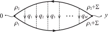
FIG. 5.: A typical ladder diagram, which describes the tunneling in the short-range random potential.

The diagram shown in Fig. 5 is of the ladder type. It is easy to see that other diagrams (with crossing dashed lines) are negligible. Indeed, consider, for instance, a diagram where $m$th and $m+1$st dashed lines of the original ladder diagram are interchanged. This diagram will be proportional to $C_{0}(\tilde{q}_{m},\Delta\rho_{y})$ where $\Delta\rho_{y}=\rho_{m,y}-\rho_{m+1,y}\sim q_{m}l^{2}$. As discussed in the preceding section, the characteristic values of $q_{m}$ are of the order of $q_{\ast}(E)$, so that the distance $\Delta\rho_{y}$ between $\rho_{my}$ and $\rho_{m+1,y}$ is of the order of $q_{\ast}(E)\,l^{2}$. This distance is much larger than $d$, the correlation length of $U_{0}$ because $l\gg d$. Therefore, $C_{0}(\tilde{q}_{m},\Delta\rho_{y})$, and thus, the entire diagram are small.

Note also that the neglect of the resonant tunneling configurations is assured by omitting the diagrams with dashed lines connecting two points of the same solid line (either the upper or the lower one).

The magnitude of the ladder diagram in Fig. 5 is equal to

                                                                                 

$$\langle|G^{(M)}|^{2}\rangle_{\rm nr}=\int\!\!\int\!\frac{d\rho_{1}d\rho_{2}}{(2\pi l^{2}E)^{2}}[\Phi_{N}(\rho_{1})\,\Phi_{N}(\rho_{2})][\Phi_{N}(\rho_{1}+\Sigma-y)\,\Phi_{N}(\rho_{2}+\Sigma-y)]\int\!\!\ldots\!\!\int\!\!\prod_{m=1}^{M}\frac{dq_{m}}{2\pi E^{2}}\,C_{0}\left(\tilde{q}_{m},\rho_{2}-\rho_{1}\right).$$ (55)

                                                                               

The products of functions $\Phi_{N}$ in the square brackets can be replaced by the integrals over auxiliary variables according to the formula

$$\Phi_{N}(x+\frac{y}{2})\,\Phi_{N}(x-\frac{y}{2})=\int\!\frac{dz}{2\pi l^{2}}\,e^{izx/l^{2}}\,F_{N}(z,y),$$ (56)

where $F_{N}(z,y)=F_{N}(\sqrt{z^{2}+y^{2}})$, which enables one to obtain a rather simple expression,

$$\langle|G^{(M)}|^{2}\rangle_{\rm nr}=\int\!\frac{d^{2}\rho\,F_{N}^{2}(\rho)}{(2\pi l^{2})^{3}}\,\frac{C_{0}(\rho)^{M}\,e^{i\rho_{x}y/l^{2}}}{E^{2M+2}},$$ (57)

and finally,

$$\langle|G(0,y;E)|^{2}\rangle_{\rm nr}=\int\!\frac{d^{2}\rho\,F_{N}^{2}(\rho)}{(2\pi l^{2})^{3}}\,\frac{e^{i\rho_{x}y/l^{2}}}{E^{2}-C_{0}(\rho)}.$$ (58)

A very similar calculation gives

$$\langle|G_{\rho}(0,y;E)|^{2}\rangle_{\rm nr}=L_{x}\int\!\frac{d\rho}{(2\pi l^{2})^{2}}\,\frac{e^{i\rho y/l^{2}}}{E^{2}-C_{0}(\rho)}.$$ (59)

Since the integrands in these formulas oscillate the more rapidly the larger $y$ is, the square modulus of the two Green’s functions decays with $y$. Furthermore, comparing Eqs. (58) and (59), we see that the decay rate of $G$ and $G_{\rho}$ is the same, i.e., that $\xi_{2}$ would not change if $G$ were replaced by $G_{\rho}$ in Eq. (54). In both cases $\xi_{2}$ is given by

$$\xi_{2}=l^{2}/v_{\ast},$$ (60)

where $v_{\ast}$ is the smallest positive root of the equation

$$C_{0}(2iv_{\ast},0)\equiv\int\!\frac{dq_{x}dq_{y}}{(2\pi)^{2}}\,C_{0}(\tilde{q}_{x},\tilde{q}_{y})\,e^{2q_{x}v_{\ast}}=E^{2}.$$ (61)

Using Eqs. (15) and (44), and also the asymptotic formula $[F_{N}(ql^{2})]^{2}\simeq 1/(\pi qR_{c})$ (valid for $N\gg 1$ and $q\ll k_{F}$) we obtain

$$\int\limits_{0}^{\infty}\!\frac{dq}{\pi R_{c}(4\pi qv_{\ast})^{1/2}}\,e^{-\frac{1}{\beta}(qd)^{\beta}+2qv_{\ast}}\simeq\frac{E^{2}}{\tilde{C}(0)}.$$ (62)

If $\beta>1$, the integrand has the saddle-point at $q=q_{\ast}$ [Eq. (46)] with the characteristic spread of $q$ around $q_{\ast}$ being $\Delta q\sim 1/\{d\,[\ln(E/W)]^{(\beta-2)/2\beta}\}$. Using the saddle-point method estimate for the integral, and then solving the resulting transcendental equation, we obtain

$$v_{\ast}\simeq\left(\frac{2\beta}{\beta-1}\ln\frac{|E|}{W}\right)^{\frac{\beta-1}{\beta}}\frac{d}{2}.$$ (63)

As one can see from Eqs. (60) and (63), the derivation of Eq. (16) will be complete if we demonstrate that $\xi_{2}=\xi$, i.e., that $\ln\langle|G(0,y;E)|^{2}\rangle_{\rm nr}-\langle\ln|G(0,y;E)|^{2}\rangle=o(y)$. (Note that we are interested mainly in the case $|E|=\hbar\omega_{c}/2$). Since such a calculation is not an easy task, we will only show that this relation holds for $G^{(M)}$, where $M\approx y/(q_{\ast}l^{2})$. Such $M$ give dominant contribution to $\langle|G(0,y;E)|^{2}\rangle_{\rm nr}$, and presumably, to $\langle\ln|G(0,y;E)|^{2}\rangle$ as well.

To average the logarithm, we employ the replica trick,

$$\langle\ln|G|\rangle=\lim_{n\to 0}\frac{\langle|G|^{2n}\rangle-1}{2n}.$$ (64)

Under the same kind of approximations as above and for integer $n$, $\langle|G^{(M)}|^{2n}\rangle_{\rm nr}$ is given by

$$\langle|G^{(M)}|^{2n}\rangle_{\rm nr}=\int\ldots\int\!\prod_{m=1}^{2n}\frac{d\rho_{m}}{2\pi l^{2}E}\Phi_{N}(\rho_{m})\,\Phi_{N}(\rho_{m}+\Sigma_{m}-y)\int\ldots\int\!\prod_{k=1}^{M}\prod_{r=1}^{n}\frac{dq_{k}^{(r)}}{2\pi E^{2}}\sum_{P_{k}}C_{0}\left[\tilde{q}_{k}^{(r)},\rho_{ky}^{(r)}-\sigma_{ky}^{(r)}\right],$$ (65)

                                                                               

where $\Sigma_{m}=\sum_{k=1}^{M}q_{k}^{(m)}l^{2}$ and $P_{k}$ labels the permutations of the superscripts of the set $\{q_{k}^{(1)},q_{k}^{(2)},\ldots,q_{k}^{(n)}\}$. The quantity $\sigma_{ky}^{(r)}$ stands for $l^{2}[q_{1}^{P_{1}(r)}+\ldots+q_{k-1}^{P_{k-1}(r)}+\frac{1}{2}q_{k}^{P_{k}(r)}]$. There are altogether $n!$ permutations $P_{k}$ for each $k$; therefore, the complete expression is a rather complicated sum of $(n!)^{M}$ terms. However, only $n!$ terms in this sum are significant. Indeed, within the adopted approximation all the terms with $|\rho_{ky}^{(r)}-\sigma_{ky}^{(r)}|\gg d$ for at least one of $k=1,2,\ldots,M$, should be dropped. It is easy to find the difference $\rho_{ky}^{(r)}-\sigma_{ky}^{(r)}$ for the case of identical permutations $P_{1},P_{2},\ldots,P_{M}$. In this case $\rho_{ky}^{(r)}-\sigma_{ky}^{(r)}=\rho_{r}-\rho_{P_{1}(r)}$ for all $k$. Therefore, a single constraint $|\rho_{r}-\rho_{P_{1}(r)}|\lesssim d$ takes care of all the $M$ constraints above. If, on the other hand, some of $P_{k}$ are not the same, then the integration domain is much more restricted, and the value of the integral is small. Retaining only the terms corresponding to identical permutations, we immediately find that

$$\langle|G^{(M)}|^{2n}\rangle_{\rm nr}\simeq n!\,\langle|G^{(M)}|^{2}\rangle^{n}_{\rm nr}.$$ (66)

Taking the limit $n\to 0$, we obtain from here [24]

$$\langle\ln|G^{(M)}|\rangle\simeq\frac{\ln\langle|G^{(M)}|^{2}\rangle_{\rm nr}-{\bf C}}{2}.$$ (67)

We think that the same relation holds if $G^{(M)}$ is replaced by the total Green’s function, $G(0,y;E)$, and so $\xi_{2}=\xi$.

Finally, let us sketch the derivation of $\xi$ for the “white-noise” random potential, $d\ll k_{F}^{-1}$. In this limit one can replace $\tilde{C}_{0}(\mathchoice{{\hbox{\boldmath$\displaystyle q$}}}{{\hbox{\boldmath$\textstyle q$}}}{{\hbox{\boldmath$\scriptstyle q$}}}{{\hbox{\boldmath$\scriptscriptstyle q$}}})$ by $\tilde{C}(0)F_{N}^{2}(ql^{2})$ in Eq. (61), which leads to the following equation on $v_{\ast}$,

$$\frac{\tilde{C}(0)}{2\pi l^{2}}\,F_{N}^{2}(2iv_{\ast})=E^{2}.$$ (68)

The next step is to use the asymptotic formula for $F_{N}(iy)$,

$$\displaystyle F_{N}(iy) \simeq \frac{l}{\sqrt{\pi ys}}\left(\frac{y+s}{2R_{c}}\right)^{2N+1}e^{{ys}/{4l^{2}}},$$ (69)

$$s = \sqrt{y^{2}+4R_{c}^{2}},$$ (70)

valid for $y\gg k_{F}^{-1}$. This way one obtains an approximate solution for $v_{\ast}$. Finally, taking $|E|$ to be $\hbar\omega_{c}/2$, one recovers Eq. (1).

IV Long-range random potential: discrete Landau levels

In the previous section devoted to short-range random potentials, we were able to derive $\xi$ by calculating the square modulus of the Green’s function. Unfortunately, this is not possible for a long-range random potential. The physical reason is as follows.

As we have shown in Sec. II, the typical distance $\Delta\rho_{y}$ between the locations of successive scattering events is of the order of $(l^{2}/d){\cal L}$, where ${\cal L}$ is some logarithmic factor. If the random potential is long-range, $d\gg l$, then $\Delta\rho_{y}\ll d$, and so such scattering events can no longer be considered uncorrelated. One of consequences is an enhanced probability of “pinholes” discussed in Sec. II. In other words, the local decay rate of the wave functions with distance becomes very nonuniform. In its turn, the Green’s function $G(0,y;E)$, even with the resonant tunneling configurations excluded, exhibits large fluctuations between different disorder realizations so that $|\ln\langle|G(0,y;E)|^{2}\rangle|\gg|\langle\ln|G(0,y;E)|^{2}\rangle_{\rm nr}|$, or $\xi_{2}\gg\xi$.

One look at Eq. (65) is sufficient to predict that a diagrammatic calculation of $\langle\ln|G(0,y;E)|^{2}\rangle$ is bound to be very cumbersome. The task is easier within a different approximation scheme, the WKB method. Some of the formulas corresponding to this approximation have been previously worked out by Tsukada [25] and by Mil’nikov and Sokolov. [12]

Suppose we want to find the solution of the Schröedinger equation $\hat{U}_{0}\phi(\rho_{y})=E\phi(\rho_{y})$. Let us seek the solution in the form $\phi(\rho_{y})=\exp[iS(\rho_{y})]$. The action $S(\rho_{y})$ can be expanded in the series of the small parameter $l/d$. In the lowest approximation, $S(\rho_{y})$ must satisfy the Hamilton-Jacoby equation,

$\displaystyle U_{0}\left(l^{2}\frac{\partial S}{\partial\rho_{y}},\rho_{y}\right)=E,$

so that

$\displaystyle\phi(\rho_{y})\sim\exp\left[\frac{i}{l^{2}}\!\int\limits^{\rho_{y}}\!d\eta\,\rho_{x}(\eta)\right],$

where $\rho_{x}(\rho_{y})$ is a solution (generally speaking, a complex one) of the equation

$$U_{0}(\rho_{x},\rho_{y})=E.$$ (71)

The meaning of this equation is quite transparent. It is known that the motion of the guiding center in classically permitted regions is a drift along the level lines of the averaged potential $U_{0}$ (see Ref.[11]). Equation (71) means that the trajectory of the guiding center in classically forbidden regions is still a level line although obtained by analytical continuation to the three-dimensional space $\{(u,v,\rho_{y})\}$ where $u={\rm Re}\,\rho_{x}$ and $v=-{\rm Im}\,\rho_{x}$.

The WKB-type formula for the Green’s function in the guiding center representation is,

$$G_{\rho}(\rho_{1},\rho_{2};E)=\frac{i}{l^{2}}\sum_{n}\frac{{\rm sgn}(\rho_{2}-\rho_{1})}{\sqrt{\displaystyle\left[{\partial U_{0}}/{\partial\rho_{x}^{(n)}}\right]_{\rho_{y}=\rho_{1}}\left[{\partial U_{0}}/{\partial\rho_{x}^{(n)}}\right]_{\rho_{y}=\rho_{2}}}}\,\exp\left[-\frac{i}{l^{2}}\int\limits_{\rho_{1}}^{\rho_{2}}\!d\rho_{y}\,\,\rho_{x}^{(n)}(\rho_{y})\right],$$ (72)

                                                                               

where the superscript $n$ labels different solutions $\rho_{x}^{(n)}=u_{n}-iv_{n}$ of Eq. (71) in the complex half-space ${\rm sgn}\,v_{n}={\rm sgn}(\rho_{2}-\rho_{1})$. If we study the tunneling from point $(0,0)$ to $(0,y)$ where $y>0$, then this will typically be the upper half-space, $v_{n}\geq 0$. Using Eqs. (30) and (72) and neglecting all the pre-exponential factors, we obtain the following estimate for $G(0,y;E)$,

$\displaystyle G\sim\sum_{n}\exp\!\!\left[-\frac{u_{n}(0)^{2}+u_{n}^{2}(y)}{2l^{2}}-\frac{i}{l^{2}}\!\int\limits_{0}^{y}\!d\rho_{y}\,\,\rho_{x}^{(n)}(\rho_{y})\right].$

Since $U_{0}$ is a random potential, it is natural to assume that the phase factors corresponding to different $n$ in this sum are uncorrelated; therefore,

$$|G|^{2}\sim\!\sum_{n}\exp\!\!\left[-\frac{u_{n}(0)^{2}+u_{n}^{2}(y)}{l^{2}}-\frac{2}{l^{2}}\!\!\int\limits_{0}^{y}\!d\rho_{y}\,v_{n}(\rho_{y})\right].$$ (73)

Consequently, $\xi$ can be calculated as follows,

$$\frac{1}{\xi}=\min\limits_{n}\lim_{y\to\infty}\frac{1}{yl^{2}}\left[\frac{u_{n}^{2}(y)}{2}+\int\limits_{0}^{y}\!d\rho_{y}\,\,v_{n}(\rho_{y})\right].$$ (74)

It is possible to demonstrate that the first term in the square brackets is typically much smaller than the second one, which leads to

$$\xi\simeq\frac{l^{2}}{\min\limits_{n}\,\langle v_{n}\rangle},$$ (75)

where $\langle v_{n}\rangle$ is the average “height” of the $n$th level line,

$\displaystyle\langle v_{n}\rangle=\lim_{y\to\infty}\frac{1}{y}\int\limits_{0}^{y}\!d\rho_{y}\,\,v_{n}(\rho_{y}).$

The problem of calculating $\min\limits_{n}\,\langle v_{n}\rangle$ turns to be rather difficult and we have not been able to solve it exactly. However, we will give arguments that $\min\limits_{n}\,\langle v_{n}\rangle\simeq v_{\ast}$ [$v_{\ast}$ was introduced in the previous section, see Eq. (61)]. Therefore, $\xi$ is still given by formula (16). A more accurate statement is as follows. If the individual Landau levels are well resolved in the density of states, then for arbitrary range $d$ of the random potential $\xi$ can be found from the same “master” equation

$$C_{0}(2il^{2}/\xi,0)=E^{2}.$$ (76)

Let us familiarize ourselves with the properties of the equipotential contours (level lines) of the potential $U_{0}$ in the half-space $\{(u,v,\rho_{y}),v\geq 0\}$. An important property is the contour density $P(v,E)$,

$\displaystyle P(v,E)=\left\langle\sum_{n}\delta(v-v_{n})\,\delta(u-u_{n})\right\rangle$

(for isotropic random potential $U_{0}$ this quantity does not depend neither on $u$ nor on $\rho_{y}$). Function $P(v,E)$ proves to be the sum of three terms,

$$P(v,E)=P_{1}(v,E)+P_{2}(v,E)+P_{3}(E)\,\delta(v),$$ (77)

where

$$\displaystyle P_{1}(v,E) = \frac{E^{2}S^{2}}{\pi Q^{2}\sqrt{QR}}\,e^{-E^{2}/Q},$$ (78)

$$\displaystyle P_{2}(v,E) = \frac{e^{-E^{2}/Q}}{2\pi\sqrt{QR}}\left[T-S^{2}\left(\frac{1}{Q}+\frac{1}{R}\right)\right],$$ (79)

and $Q$, $R$, $S$, and $T$ are as follows,

$$\begin{array}[]{c}Q=C_{0}(2iv,0)+C_{0}(0,0),\\[12.0pt] R=C_{0}(2iv,0)-C_{0}(0,0),\\[12.0pt] S=\frac{1}{2}\,{dQ}/{dv},\>\>\>T=\frac{1}{2}\,{d^{2}Q}/{dv^{2}}.\end{array}$$ (80)

Except for the term $P_{3}(v)$ our formulas are in agreement with Refs. [14] and [26]. This term, however, does not play any role in the subsequent calculation. The derivation of Eqs. (78) and (79) can be found in the Appendix.

FIG. 6.: Functions $P_{1}(v,E)$ and $P_{2}(v,E)$. Vertical axis is in units of $1/d^{2}$. The parameters used in generating the plot are $\beta=2$ and $E/W=5$.

The behavior of functions $P_{1}$ and $P_{2}$ is illustrated by Fig. 6. Function $P_{1}$ has a sharp maximum at $v=v_{\ast}$ where $Q\simeq E^{2}$. Away from the maximum it is exponentially small. Function $P_{2}$ is exponentially small at $v<v_{\ast}$, and assumes the asymptotic form $P_{2}(v,E)\propto v^{(2-\beta)/(\beta-1)}$ at $v>v_{\ast}$. For example, if $\beta=2$, then $P_{2}(v,E)\to 1/(\pi d^{2})$ (see Fig. 6). The ratio $P_{1}/P_{2}$ evaluated at the point $v_{\ast}$ is of the order of $\ln|E/W|\gg 1$ in the case of interest. At $v$ close to $v_{\ast}$ our expression essentially coincides with Eq. (5.20) of Ref. [14]. Note however, that the latter equation is off by $4\pi$.

Let us clarify the origin of the sharp maximum in $P(v,E)$ at $v=v_{\ast}$. To this end the concept of bands of harmonics introduced in Sec. II is very helpful. So, let us consider a band with $q_{x}$ in the interval $(q-\frac{1}{2}\Delta q,q+\frac{1}{2}\Delta q)$ where $q\gg\Delta q>0$. The amplitude of each harmonic $U_{0}(\tilde{q}_{x},\rho_{y})$ is enhanced by the factor $e^{q_{x}v}$ upon the analytic continuation into the upper half-space. Therefore, the typical value of the combined amplitude $U_{q}(\mathchoice{{\hbox{\boldmath$\displaystyle\rho$}}}{{\hbox{\boldmath$\textstyle\rho$}}}{{\hbox{\boldmath$\scriptstyle\rho$}}}{{\hbox{\boldmath$\scriptscriptstyle\rho$}}})$ of the band [see Eq. (41) for definition] grows from $W_{q}(0)\sim[C_{0}(\tilde{q},0)\Delta q]^{1/2}$ at $v=0$ to $W_{q}(v)\sim[C_{0}(\tilde{q},0)\Delta q]^{1/2}\,e^{qv}$ at $v>0$. Being the product of the rapidly decreasing function $C_{0}(\tilde{q},0)$ and the exponentially growing factor $e^{qv}$, this quantity has a sharp maximum at $q=q_{\ast}(v)$,

$$q_{\ast}(v)=\frac{1}{d}\left(\frac{2v}{d}\right)^{\frac{1}{\beta-1}},$$ (81)

provided that $\beta>1$ and $v\gg d$. [In view of Eq. (63), this formula is just another parametrization of $q_{\ast}$ originally defined by Eq. (46) as a function of $E$]. Generally speaking, the width of the maximum depends on $v$ and $\beta$ but in a particular example, $\beta=2$, it is simply $\Delta q\sim\frac{1}{d}$. Hence, at a given “height” $v$ in our three-dimensional space, the potential $U_{0}(\rho_{x},\rho_{y})$ is typically dominated by the band of harmonics of width $\Delta q$ centered at $q_{\ast}(v)$. Consequently, the spatial dependence of $U_{0}$ is almost plain-wave-like, $U_{0}(\rho_{x},\rho_{y})\propto e^{i\rho_{x}q_{\ast}(v)}$. This prompts the decomposition

$$U_{0}(\mathchoice{{\hbox{\boldmath$\displaystyle\rho$}}}{{\hbox{\boldmath$\textstyle\rho$}}}{{\hbox{\boldmath$\scriptstyle\rho$}}}{{\hbox{\boldmath$\scriptscriptstyle\rho$}}})=e^{i\rho_{x}q_{\ast}(v)}V(\mathchoice{{\hbox{\boldmath$\displaystyle\rho$}}}{{\hbox{\boldmath$\textstyle\rho$}}}{{\hbox{\boldmath$\scriptstyle\rho$}}}{{\hbox{\boldmath$\scriptscriptstyle\rho$}}})$$ (82)

of $U_{0}$ into the “oscillating part” $e^{i\rho_{x}q_{\ast}(v)}$ and a “smooth part” $V(\mathchoice{{\hbox{\boldmath$\displaystyle\rho$}}}{{\hbox{\boldmath$\textstyle\rho$}}}{{\hbox{\boldmath$\scriptstyle\rho$}}}{{\hbox{\boldmath$\scriptscriptstyle\rho$}}})$.

The intersection points of the level lines $U_{0}=E$ with a vertical plane $\rho_{y}=\eta$ satisfy the system of equations

$$v_{n} = -\frac{1}{q_{\ast}(v_{n})}\ln\frac{|V|}{E},$$ (83)

$$u_{n} = \frac{1}{q_{\ast}(v_{n})}\arg V+\frac{2\pi n}{q_{\ast}(v_{n})}.$$ (84)

The modulus $|V|$ of the complex Gaussian variable $V$ has the Maxwellian distribution with the characteristic width ${\cal W}$ given by

$${\cal W}^{2}\equiv\langle|V(\mathchoice{{\hbox{\boldmath$\displaystyle\rho$}}}{{\hbox{\boldmath$\textstyle\rho$}}}{{\hbox{\boldmath$\scriptstyle\rho$}}}{{\hbox{\boldmath$\scriptscriptstyle\rho$}}})|^{2}\rangle\simeq e^{-2vq_{\ast}(v)}Q,$$ (85)

where $Q$ is defined by Eq. (80). In the first approximation let us neglect the dependence of $V$ on $\rho_{x}$, (which corresponds to the limit of infinitesimally narrow band, $\Delta q\to 0$), then $P(v,E)$ is given by

$\displaystyle P(v,E)=\frac{q_{\ast}}{2\pi}\!\int\limits_{0}^{\infty}\frac{2|V|\,d|V|}{{\cal W}^{2}}\,e^{-|V|^{2}/{\cal W}^{2}}\delta\!\left(\!v+\frac{1}{q_{\ast}}\ln\frac{|V|}{\cal W}\right),$

Doing the integration, we arrive at

$$P(v,E)=\frac{E^{2}q_{\ast}^{2}(v)}{\pi Q}e^{-E^{2}/Q},$$ (86)

which, in fact, coincides with $P_{1}(v,E)$ provided that $v\gg d$. In this approximation $u_{n}$ form an equidistant set, $u_{n+1}-u_{n}\simeq 2\pi/q_{\ast}\ll 1/d$, while $v_{n}$ does not depend on $n$. The equipotential contours resemble a number of uniformly spaced parallel rods, which “soar” above the real plane $v=0$, staying very close to the “standard height” $v=v_{\ast}$ for most values of $\rho_{y}$. Indeed, as discussed above (see also Fig. 6), function $P_{1}$ has a sharp maximum at $v=v_{\ast}$. Since $d\ln Q/dv\simeq 2q_{\ast}$, the width of the maximum is of the order of $1/q_{\ast}$. This is, of course, can be seen directly from Eq. (83): if $|V|$ has its typical value, ${\cal W}$, then $v_{n}=v_{\ast}$. Fluctuations of $|V|$ change the logarithm (typically) by a number of the order of unity; therefore, ordinarily $|v_{n}-v_{\ast}|\simeq 1/q_{\ast}$. Significant deviations from the “standard height” $v_{\ast}$ are exponentially rare.

We believe that such a description accurately portrays the behavior of the relevant equipotential contours in the upper half-space, which means that $\langle v_{n}\rangle\simeq v_{\ast}$ for such contours, and therefore, $\xi$ is given by the old formula (16).

As one can see from Eqs. (77-79) and (86), our approximate treatment does not capture the term $P_{2}(v,E)$ in $P(v,E)$, which seems to be important for $v>v_{\ast}$. Therefore, the possibility of $\min_{n}\langle v_{n}\rangle$ being larger than $v_{\ast}$ can not be totally ignored. Although we can not rigorously prove that $\min_{n}\langle v_{n}\rangle=v_{\ast}$, we managed to find the upper bound for $\min_{n}\langle v_{n}\rangle$,

$$\min\limits_{n}\langle v_{n}\rangle<v_{\ast}+O(1)\,d,$$ (87)

based on the following percolation-type arguments.

Suppose that there exists a level line number $m$, $U_{0}[\rho_{x}^{(m)},\rho_{y}]=E$, which is totally contained in a slab $\{(u,v,\rho_{y}),0\leq v\leq v_{0}\}$. In this case $\min_{n}\langle v_{n}\rangle\leq\langle v_{m}\rangle\leq v_{0}$. This prompts considering the following percolation problem. Let us call “wet” all the points $(u,v,\rho_{y})$ of the slab, which satisfy the conditions

$\displaystyle{\rm Re}\,U_{0}(u-iv,\rho_{y})\leq E,\quad{\rm Im}\,U_{0}(u-iv,\rho_{y})\leq 0.$

As the thickness $v_{0}$ of the slab increases from zero, it should eventually reach a critical value $v_{c}$, at which the percolation through “wet” regions first appears. The percolation threshold $v_{c}$ is at the same time the upper bound for $\min\limits_{n}\langle v_{n}\rangle$.

Obviously, no percolation exists for $v_{0}<v_{\ast}$ when the wet regions occupy exponentially small fraction of the volume. On the other hand, if $v_{0}\gg v_{\ast}$, then $\langle({\rm Re}\,U_{0})^{2}\rangle\simeq\langle({\rm Im}\,U_{0})^{2}\rangle\simeq Q/2\gg E^{2}$, and approximately a quarter of the entire volume is wet. This greatly exceeds the volume fraction $0.17$ required for the percolation in continual three-dimensional problems; [18] thus, such $v_{0}$ are high above the percolation threshold. Furthermore, the relation between the percolation thresholds of the continuum and of a film [27] suggests that $v_{c}$ must be equal to $v_{\ast}+Cd$, where $C\sim 1$, which leads to Eq. (87).

Finally, let us comment on the relation of our approach to that of Raikh and Shahbazyan [14] already mentioned above. In Ref. [14] the idea of the complex trajectories $\rho_{x}^{(n)}(\rho_{y})=u_{n}(\rho_{y})-iv_{n}(\rho_{y})$, which is the basis of our calculation of the Green’s function, was introduced. However, an approximation early in their analysis [dropping of the cross-product in Eq. (2.8) of Ref. [14]] led the authors of Ref. [14] to the result, which in our notations can be written as follows:

$\displaystyle G_{\rho}(0,y;E)=\frac{i}{l^{2}}\sum_{n}\,[{\partial U_{0}}/{\partial\rho_{x}^{(n)}}]^{-1}\exp\!\left[\frac{i}{l^{2}}\,y\,\rho_{x}^{(n)}(y/2)\right]$

(the derivative is taken at $\rho_{y}=y/2$). As one can see, in their method $G_{\rho}(0,y;E)$ is determined not by the entire tunneling trajectory, as it should [see Eq. (72)], but only by its midpoint $\rho_{y}=y/2$. As a result, the point-to-point Green’s function $G(0,y;E)$ obtained by their method starts to be in error strictly speaking already for $y\gtrsim d$. The only case where the method of Raikh and Shahbazyan [14] works for arbitrary $y$ is the case of a one-dimensional potential, e.g., $U_{0}(x,y)=U_{0}(x)$. A potential of this type has the same magnitude at the midpoint $y/2$ and at all other points $y$. (From the formal point of view, only for this type of potentials the aforementioned cross-product vanishes for any $y$ and therefore can be dropped).

The reduction of the properties of the entire trajectory to the properties of a single point destroys the self-averaging of the localization length, which is a well established property of other disordered systems. [22] Because of that, it becomes necessary to treat $\xi$ as a function of $y$. As we mentioned above, for a given disorder realization the value of $G(0,y;E)$ given by the formulas of Ref. [14] is in error already for $y\gtrsim d$. However, this is not so for the quantity $\langle\ln|G(0,y;E)|\rangle$. The logarithmic averaging manages to mask the error so that $\xi(y)$ remains close to the correct asymptotic value given by Eq. (16) for sufficiently short distances, $y\ll d\,\exp(E^{2}/W_{0}^{2})$. Indeed, if one uses the last equation above, then one obtains

$\displaystyle|G|^{2}\sim\sum_{n}\exp\left\{-\frac{2}{l^{2}}\left[u_{n}^{2}(y/2)+y\,v_{n}(y/2)\right]\right\},$

instead of Eq. (73) and

$$\frac{1}{\xi(y)}\simeq\frac{1}{l^{2}}\min\limits_{n}\left[\frac{u_{n}^{2}(y/2)}{y}+v_{n}(y/2)\right]$$ (88)

instead of Eq. (74). If $y\ll d\,\exp(E^{2}/W_{0}^{2})$, the minimum is typically supplied by one of the trajectories whose “height” $v_{n}$ is not too different from the standard value of $v_{\ast}$, $|v_{n}-v_{\ast}|\lesssim d$. This range of $v_{n}$ allows for $u_{n}$ in the range $|u_{n}|\lesssim\sqrt{yd}$. Therefore, the optimal trajectory is typically one of about $M=\sqrt{y/d}$ trajectories closest to the $x=0$ axis. Note that $M$ increases with $y$. Eventually, at $y\sim d\,\exp(E^{2}/W_{0}^{2})$ it becomes exponentially large so that there is an appreciable probability that one out of such $M$ trajectories has $v_{n}(y/2)<v_{\ast}/2$ and $|u_{n}(y/2)|^{2}<yd/2$. The decay rate $1/\xi(y)$ in this case is determined by such an untypical trajectory, and so $\xi(y)$ is significantly larger than our result, Eq. (16). Furthermore, at $y\gg d\,\exp(E^{2}/W_{0}^{2})$, there is a finite probability of finding $v_{n}(y/2)$ exactly equal to zero [due to the third term in Eq. (77)]. Therefore, in the asymptotic limit $y\to\infty$ the method of Raikh and Shahbazyan [14] yields a very surprising result $1/\xi(y)\to 0$. As we explained above, this is a consequence of an effective substitution of the original two-dimensional random potential by a potential depending on a single coordinate.

V Overlapping Landau levels

This section is devoted to the derivation of Eq. (1). An important difference from all the preceding calculations is that the potential energy $E=E_{F}-\hbar\omega_{c}(N+\frac{1}{2})$ is smaller than the amplitude $W_{0}$ of the averaged potential $U_{0}(\mathchoice{{\hbox{\boldmath$\displaystyle\rho$}}}{{\hbox{\boldmath$\textstyle\rho$}}}{{\hbox{\boldmath$\scriptstyle\rho$}}}{{\hbox{\boldmath$\scriptscriptstyle\rho$}}})$. In this case the level lines $U_{0}[\rho_{x}^{(n)},\rho_{y}]=E$ introduced in Sec. IV, stay predominantly in the real plane $v=0$. [Their density is given by $P_{3}(v,E)$, see Eq. (77)]. However, for $E\neq 0$ the percolation of the level lines in the $y$-direction discussed in the end of the previous section, still requires brief excursions into the upper complex half-space. Such excursion link together the large closed loop contours $U_{0}=E$ of typical diameter $\xi_{\rm perc}(E)$. The localization length $\xi$ is still given by Eq. (75), which leads to the estimate

$$\xi\sim\frac{l^{2}}{\langle v\rangle_{\rm ex}}\,\frac{\xi_{\rm perc}(E)}{\Delta\rho},$$ (89)

where the subscript “ex” indicates that the averaging is performed only over the “excursions”, i.e., over the parts with $v>0$, with $\Delta\rho$ being the typical length of such parts. Similar to the case $N=0$ discussed previously by Mil’nikov and Sokolov, [12] $\langle v\rangle_{\rm ex}\sim\Delta\rho\sim(|E|/U_{0}^{\prime\prime})^{1/2}$ where $U_{0}^{\prime\prime}\sim W_{0}/d^{2}$ is the typical value of the second derivatives of the averaged potential $U_{0}$; therefore,

$$\xi\sim\xi_{\rm perc}(E)\,\frac{W_{0}l^{2}}{Ed^{2}}.$$ (90)

The calculation of the quantity $\xi_{\rm perc}(E)$ is a subject of statistical topography, [18] and the following results are established. Denote by $C_{\lambda}$ the integral,

$\displaystyle C_{\lambda}\equiv\int\limits_{\frac{1}{2}<|q|\lambda<1}\!\!\!\!\!\frac{d^{2}q}{(2\pi)^{2}}\,\tilde{C}_{0}(q).$

For slowly decaying correlators $\tilde{C}_{0}(q)$, such that $C_{\lambda}\sim\lambda^{-2H}$ with $H\leq 3/4$, $\xi_{\rm perc}$ is given by (besides the review, Ref. [18], see the original works, Ref. [28]),

$$\xi_{\rm perc}(E)\sim d\,|W_{0}/E|^{1/H}.$$ (91)

Otherwise, i.e., if $C_{\lambda}$ decays faster than $\lambda^{-3/2}$, then [18]

$$\xi_{\rm perc}(E)\sim d\,|W_{0}/E|^{4/3}.$$ (92)

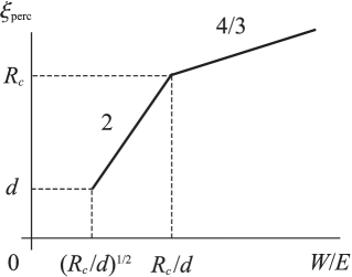
FIG. 7.: The percolation length $\xi_{\rm perc}$ as a function of the energy $E$ (schematically). The labels “2” and “4/3” indicate the power-law exponents in the corresponding intervals, see Eq. (93).

Let us now determine the conditions under which formulas (91) and (92) become applicable. The issue is complicated by the fact that $\tilde{C}_{0}(q)$ is the product of two terms, $\tilde{C}_{0}(q)$ and $[F_{N}(ql^{2})]^{2}$, see Eq. (44). The former decays exponentially starting from $q\sim 1/d$. The latter remains close to one at $q\lesssim 1/R_{c}$, then behaves according to a power-law, $[F_{N}(ql^{2})]^{2}\sim 1/q$ for $1/R_{c}<q<2k_{F}$, and finally, decays exponentially at $q>2k_{F}$. Such a complicated behavior results into three different regimes (1a-c).

The simplest is the case $R_{c}\ll d$, where $[F_{N}(ql^{2})]^{2}\simeq 1$ for all relevant $q$. In this case Eq. (92) applies and also $W_{0}\simeq W$. The localization length is given by Eq. (1a), which coincides with the result of Mil’nikov and Sokolov. [12]

If $R_{c}\gg d$, then the situation is more complicated. In this case $C_{\lambda}$ is proportional to $1/\lambda$, i.e., $H=\frac{1}{2}$ for $d\ll\lambda\ll R_{c}$, yet decays faster than $1/\lambda^{3/2}$ for $\lambda>R_{c}$. As a result, both Eq. (91) and Eq. (92) for $\xi_{\rm perc}$ may apply, depending on $E$,

$$\xi_{\rm perc}(E)\sim\left\{\begin{array}[]{lc}\displaystyle\frac{d^{2}}{R_{c}}\left|\frac{W}{E}\right|^{2},&\displaystyle\frac{d}{R_{c}}<\frac{|E|}{W}<\sqrt{\frac{d}{R_{c}}},\\[12.0pt] \displaystyle R_{c}\left|\frac{d}{R_{c}}\frac{W}{E}\right|^{\frac{4}{3}},&\displaystyle|E|<W\frac{d}{R_{c}},\end{array}\right.$$ (93)

which is illustrated by Fig. 7. Combining Eq. (90) where $W_{0}\sim W\sqrt{d/R_{c}}$ with Eq. (93) and using $|E|=\hbar\omega_{c}/2$, one obtains Eqs. (1b) and (1c).

VI Discussion of a more realistic model and its comparison with the experiment

To make the connection with the experimental practice we will consider the model where the random potential is created by randomly positioned ionized donors with two-dimensional density $n_{i}$ set back from the electron gas by an undoped layer of width $d$. We will assume that $1/d^{2}\ll n_{i}\ll n^{2}d^{2}$. In zero magnetic field the random potential can be considered a weak Gaussian random potential with the correlator

$$\tilde{C}(q)=\pi^{2}n_{i}(e^{2}a_{B})^{2}\,e^{-2qd},$$ (94)

where $a_{B}=\hbar^{2}\kappa/me^{2}$ is the effective Bohr radius (see Appendix B of Ref. [11]). This formula corresponds to $\beta=1$ and $d$ replaced by $2d$ in Eq. (15). Deriving Eq. (94), we took into account the screening of the donors’ potential by the electron gas described by the dielectric function [8]

$$\varepsilon(q)=\kappa\left(1+\frac{2}{a_{\rm B}q}\right),\quad q\leq 2k_{F}.$$ (95)

This model remains to be accurate in sufficiently weak fields, where the Landau levels overlap and the density of states is almost uniform, like in zero field. In stronger fields (the boot-shaped region AHIGEB in Fig. 1), the density of states develops sharp peaks at the Landau level centers separated by deep minima. This strongly influences the property of the electron gas to screen the external impurity potential. Different aspects of such a screening in weak magnetic fields have been addressed in Refs. [29, 30, 31]. The screening can be be both linear and nonlinear, depending on the wave vector $q$.

The concept of nonlinear screening has been developed by Shklovskii and Efros initially for the three-dimensional case. [7] Gergel and Suris [32] have extended it to the two-dimensional case. The influence of a strong magnetic field on the nonlinear screening has been studied in Ref. [33] and especially in Ref. [34].

Nonlinear screening is realized for sufficiently small $q$, $q<q_{\rm nonl}$, and is enhanced compared to the zero field case [Eq. (95)]. The threshold wave vector $q_{\rm nonl}$ is a complicated function of the magnetic field. [31] If $q_{\rm nonl}$ is smaller than $1/R_{c}$, there exists an intermediate range of $q$, $q_{\rm nonl}<q<1/R_{c}$, where the screening remains in the linear regime but is suppressed compared to Eq. (95). The corresponding dielectric function is given by [29, 30]

$$\varepsilon(q)\simeq\kappa\left(1+\frac{R_{c}^{2}q}{a_{\rm B}}\right).$$ (96)

At even larger $q$, $q>\max\{q_{\rm nonl},1/R_{c}\}$, there is no essential change in the screening properties brought about by the magnetic field.

Clearly, in such magnetic fields the model of a Gaussian random potential with the correlator (94) becomes an oversimplification. Fortunately, the localization length $\xi$ should not be strongly affected by this. Indeed, $\xi$ is sensitive only to the combined amplitude of the narrow band of harmonics with wave vectors $q\simeq q_{\ast}$. It can be shown that for $\beta$ equal to one, $q_{\ast}\simeq 2k_{F}$ (just like for the “white-noise” potential). This wave vector belongs to the last group of $q$ for which there is no change in the screening properties. In fact, at such $q$ the screening is equally ineffective both in zero and in arbitrary strong magnetic field, $\varepsilon(2k_{F})\simeq\kappa$.

The parameter $k_{F}d$ is almost always larger than one in the experiment; therefore, in strong fields $\xi$ is expected to be given by Eq. (16). For $\beta=1$ this formula becomes remarkably simple,

$\displaystyle\xi\simeq\frac{l^{2}}{d}=\frac{R_{c}}{k_{F}d}.$

The simplest way to obtain this expression is to start with Eq. (16) for $\beta>1$, take the limit $\beta\to 1$, and then make a replacement $d\to 2d$ (see above). For $k_{F}d$ close to unity, however, one should use a refined formula

$$\xi\simeq\frac{R_{c}}{k_{F}d+\frac{1}{2}\ln(\hbar\omega_{c}/W_{0})},$$ (97)

which follows from the master equation (76). Formula (97) should hold in the boot-shaped region AHIGEB of Fig. 1. The corresponding range of $N$ can be expressed in terms of the dimensionless parameters $k_{F}d$ and $n_{i}/n$. We will concentrate on the case $n_{i}\sim n$, which we call “standard.” In this case Eq. (97) is valid for $N\lesssim 2k_{F}d$. At larger $N$, the localization length is given by Eq. (1) so that the dependence of $\xi$ on $\nu$ is super-linear. Note that the “standard” case corresponds to the straight-line “trajectory” passing through the points E and F and shown by the arrows in Fig. 1. Between these points, Eq. (1) reduces to

$$\frac{\xi}{R_{c}}\sim\frac{N^{3/2}}{(k_{F}d)^{5/2}},\quad 2k_{F}d\lesssim N\lesssim C(k_{F}d)^{5/3},$$ (98)

where $C$ is some undetermined numerical factor. At even larger $N$, $\xi$ becomes exponentially large, which precludes its accurate measurement at experimentally accessible temperatures. For this reason we do not give the explicit formula for the localization length at such $N$.

Unfortunately, the published experimental data on the low-temperature magnetoresistance away from the QHE peaks is limited to the measurements done by Ebert et al. [3] more than a decade ago. In most of their samples $d$ was equal to 6 nm, which corresponds to $k_{F}d=0.9$. On the one hand, this places the samples close to the line HI in Fig. 1. On the other hand, the “standard” case corresponds to the line EF. In fact, there is no contradiction here because in the “standard” case $E_{F}/W\sim k_{F}d$. Therefore, the as $k_{F}d$ tends to unity, the boot-shaped region AHIGEB shrinks and the lines EF and HI become quite close.

With the help of Eq. (4), we converted $T_{0}$ reported by Ebert et al. [3] into $\xi$. Only even $\nu$ were selected for this analysis. The constant factor in Eq. (4) was chosen to be $6.0$ following Nguyen. [35] For filling factors $\nu=2$ and $\nu=4$, i.e., $N=1$ and $N=2$, there is a good agreement with Eq. (97) if the logarithm in the denominator is neglected. At larger $\nu$, $6\leq\nu\leq 12$, empirical $\xi$ behaves roughly like

$$\xi\approx 2.2N^{3/2}R_{c}.$$ (99)

Formally, this is in agreement with Eq. (98). However, since the parameter $k_{F}d$ is close to one, the random potential can not be treated as long-range, and so the percolation picture used in derivation of Eq. (98) is not quite justified. Perhaps, it is more resonable to treat Eq. (99) as an approximation to the exponential dependence, Eq. (8), within a limited range of $\nu$.

Another comment is in order here. Formula (4) is based on the assumption that the interaction energy of two quasiparticles separated by a typical hopping distance $r$ is given by the Coulomb law. As was shown in Ref. [30], with a dielectric function given by Eq. (96), the Coulomb law is realized only at sufficiently large distances, $r\gg R_{c}^{2}/a_{B}$. Large hopping distances $r$ correspond to low temperatures, $T=(\xi/4r)^{2}T_{0}$. Therefore, formula (4) is expected to hold only for

$$T<\left(\frac{a_{B}\xi}{4R_{c}^{2}}\right)^{2}T_{0}.$$ (100)

Experimentally, such low temperatures may be hard to reach, especially in weak fields where $R_{c}$ is large. Therefore, we think that a different type of measurement may be more promising. One has to measure both the temperature and the current dependence of the magnetoresistance. Comparing the results of these two types of measurements, one can determine the effective temperature $T_{\rm eff}$ for each value of the current density $j$. As discussed in Ref. [6], the relation between $T_{\rm eff}$ and $j$ is as follows,

$$k_{B}\,T_{\rm eff}(j)\simeq 0.5\,ej\rho_{xy}\,\xi,$$ (101)

where $\rho_{xy}$ is the Hall resistivity. Equation (101) does not involve the dielectric function and therefore, is expected to hold even when Eq. (3) and the corresponding current dependence [6] $\rho_{xx}\propto e^{-\sqrt{T_{0}/T_{\rm eff}(j)}}$ do not match the magnetoresistance data exactly.

A Level line density $P(v,E)$

The equation $U_{0}=E$ is equivalent to the system of two equations $R=E$ and $I=0$, where $R={\rm Re}\,U_{0}(u-iv,\rho_{y})$ and $I=-{\rm Im}\,U_{0}(u-iv,\rho_{y})$. To calculate $P(v,E)$ we need to know the Jacobian $J=|\partial(R,I)/\partial(u,v)|$. With the help of the Cauchy relations,

$\displaystyle\partial R/\partial v=\partial I/\partial u,\>\>\>\partial R/\partial u=-\partial I/\partial v,$

the Jacobian can be written as

$\displaystyle J=R_{v}^{2}+I_{v}^{2},$

where subscripts denote the partial derivatives. Therefore, for all $v\neq 0$,

$$\displaystyle P(v,E) = \int\!\frac{dR\,dR_{v}\,dI\,dI_{v}}{(2\pi)^{2}(\det{\sf K})^{1/2}}\,\delta(R-E)\,\delta(I)\,(R_{v}^{2}+I_{v}^{2})$$ (A1)

$$\times \exp\left(-\frac{1}{2}{\bf v}^{T}{\sf K}^{-1}{\bf v}\right),$$ (A2)

where ${\bf v}$ is the four-component vector $(R,R_{v},I,I_{v})^{T}$ and ${\sf K}$ is its autocorrelation matrix, ${\sf K}_{mn}=\langle v_{m}v_{n}\rangle$. Matrix ${\sf K}$ turns out to be block-diagonal, the blocks being $2\times 2$ matrices. Matrix elements of ${\sf K}$ can be calculated using Eq. (5). For example, the upper diagonal block has elements ${\sf K}_{11}=Q/2$, ${\sf K}_{12}={\sf K}_{21}=S/2$, and ${\sf K}_{22}=R/2$ [see Eq. (80) for definitions]. The subsequent integration over $R_{v}$ and $I_{v}$ in formula (A2) becomes a trivial task and yields the result represented by Eqs. (78) and (79).

The case $v=0$ requires a special consideration because the condition $I=0$ is satisfied identically. It is easy to see that a level line would typically branch upon the intersection with the $v=0$ plane. The additional branch or branches are totally contained in this plane, which gives the delta-function-like contribution to function $P(v,E)$. The coefficient in front of the delta-function is given by

$$\displaystyle P_{3}(E) = \int\!\frac{dR\,dI_{v}}{2\pi({\sf K}_{11}{\sf K}_{44})^{1/2}}\,\delta(R-E)\,|I_{v}|$$

$$\times \exp\left[-(R^{2}/2{\sf K}_{11})-(I_{v}^{2}/2{\sf K}_{44})\right]$$

$$= \frac{1}{4\pi}\sqrt{-\frac{{\nabla}^{2}C_{0}(0)}{C_{0}(0)}}\,e^{-E^{2}/2W_{0}^{2}}.$$

As expected, $P_{3}(E)$ is exponentially small for $|E|\gg W_{0}$.

REFERENCES

- [1] The Quantum Hall Effect, edited by R. E. Prange and S. M. Girvin (Springer-Verlag, New York, 1990).
- [2] See B. Huckestein, Rev. Mod. Phys. 67, 347 (1995) and references therein.
- [3] G. Ebert, K. v. Klitzing, C. Probst, E. Schuberth, K. Ploog, and G. Weimann, Solid State Commun. 45, 625 (1983); G. Ebert, Ph.D. thesis (Max Planck Institute, Stuttgart, 1983).
- [4] A. Briggs, Y. Guldner, J. P. Veiren, M. Voos, J. P. Hirtz, and M. Razeghi, Phys. Rev. B27, 6549 (1983).
- [5] V. J. Goldman and L. P. Rokhinson (unpublished).
- [6] D. G. Polyakov and B. I. Shklovskii, Phys. Rev. Lett.70, 3796 (1993).
- [7] B. I. Shklovskii and A. L. Efros, Electronic properties of doped semiconductors (Springer-Verlag, Berlin, 1984).
- [8] See T. Ando, A. B. Fowler, and F. Stern, Rev. Mod. Phys. 54, 437 (1982) and references therein.
- [9] M. E. Raikh and T. V. Shahbazyan, Phys. Rev. B47, 1522 (1993).
- [10] B. Laikhtman and E. L. Altshuler, Ann. Phys. 232, 332 (1994).
- [11] M. M. Fogler, A. Yu. Dobin, V. I. Perel, and B. I. Shklovskii, Phys. Rev. B(in press).
- [12] G. V. Mil’nikov and I. M. Sokolov, Pis’ma Zh. Eksp. Teor. Fiz. 48, 494 (1988) [JETP Lett. 48, 536 (1988)].
- [13] A conceptually similar problem has been considered by B. I. Shklovskii in Fiz. Tv. Tela 26, 585 (1984) [Sov. Phys. - Solid State 26, 353 (1984)].
- [14] M. E. Raikh and T. V. Shahbazyan, Phys. Rev. B51, 9682 (1995).
- [15] B. I. Shklovskii and A. L. Efros, Zh. Eksp. Teor. Fiz. 84, 811 (1983) [Sov. Phys. JETP 57, 470 (1983)].
- [16] Q. Li and D. J. Thouless, Phys. Rev. B40, 9738 (1989).
- [17] B. I. Shklovskii, Pis’ma Zh. Eksp. Teor. Fiz. 36, 43 (1982) [JETP Lett. 36, 51 (1982)].
- [18] See the review paper, M. B. Isichenko, Rev. Mod. Phys. 64, 961 (1992), and the references therein.
- [19] J. Haidu, M. E. Raikh, and T. V. Shahbazyan, Phys. Rev. B50, 17 625 (1994)
- [20] D. J. Thouless, J. Phys. C 5, 77 (1972).
- [21] F. J. Dyson, Phys. Rev. 92, 1331 (1953).
- [22] E. M. Lifshitz, S. A. Gredeskul, and L. A. Pastur, Introduction to The Theory of Disordered Systems (Wiley, New York, 1988).
- [23] Note that the quantity diverges like as . Therefore, the average square modulus of the exact Green’s function is infinite. The quantity we calculate, is perfectly finite and can be used to get meaningful results for .
- [24] Note that our estimate for the difference between and is much smaller than the value obtained in Ref.[15], although no rigor in the derivation of this quantity in Ref.[15] is claimed. The likely reason for the disagreement is the unwarranted replacement of each “scattering region” introduced in that work by an effective single scatterer.
- [25] M. Tsukada, J. Phys. Soc. Jpn. 41, 1466 (1976).
- [26] T. V. Shahbazyan, private communication.
- [27] B. I. Shklovskii, Phys. Lett. A 51, 289 (1975); A. V. Sheinman, Fiz. Tekh. Polupr. 9, 2146 (1975) [Sov. Phys. – Semicond. 9, 1396 (1975)].
- [28] A. Weinrib and B. I. Halperin, Phys. Rev. B27, 413 (1983); A. Weinrib, ibid. 29, 387 (1984).
- [29] I. V. Kukushkin, S. V. Meshkov, and V. B. Timofeev, Usp. Fiz. Nauk 155, 219 (1988) [Sov. Phys. Usp. 31, 511 (1988)]
- [30] I. L. Aleiner and L. I. Glazman, Phys. Rev. B52, 11 296 (1995).
- [31] M. M. Fogler and B. I. Shklovskii (unpublished). An incomplete account of this work can be found in Phys. Rev. B52, 17 366 (1995).
- [32] V. A. Gergel and R. A. Suris, Zh. Eksp. Teor. Fiz. 75, 191 (1978) [Sov. Phys. JETP 48, 95 (1978)].
- [33] B. I. Shklovskii and A. L. Efros, Pis’ma Zh. Eksp. Teor. Fiz. 44, 520 (1986) [JETP Lett. 44, 669 (1986)].
- [34] A. L. Efros, Solid State Commun. 65, 1281 (1988); 67, 1019 (1989); 70, 253 (1989).
- [35] Nguyen Van Lien, Fiz. Tekh. Polupr. 18, 335 (1984) [Sov. Phys. Semicond. 18, 207 (1984)].