The Loop Algorithm

Abstract

A review of the Loop Algorithm, its generalizations, and its relation to some other Monte Carlo techniques is given. The loop algorithm is a Quantum Monte Carlo procedure which employs nonlocal changes of worldline configurations, determined by local stochastic decisions. It is based on a formulation of quantum models of any dimension in an extended ensemble of worldlines and graphs, and is related to Swendsen-Wang algorithms. It can be represented directly on an operator level, both with a continuous imaginary time path integral and with the stochastic series expansion (SSE). It overcomes many of the difficulties of traditional worldline simulations. Autocorrelations are reduced by orders of magnitude. Grand-canonical ensembles, off-diagonal operators, and variance reduced estimators are accessible. In some cases, infinite systems can be simulated. For a restricted class of models, the fermion sign problem can be overcome. Transverse magnetic fields are handled efficiently, in contrast to strong diagonal ones. The method has been applied successfully to a variety of models for spin and charge degrees of freedom, including Heisenberg and XYZ spin models, hard-core bosons, Hubbard, and $t$-$J$-models. Due to the improved efficiency, precise calculations of asymptotic behavior and of quantum critical exponents have been possible.

Contents

toc

1 Introduction and Summary

A pedagogical review of the loop algorithm, its generalizations, and the range of present applications is given, including some new results. The loop algorithm [1, 2, 3, 4] is a Quantum Monte Carlo procedure. It is applicable to numerous models both in imaginary time worldline formulation [5] and within the stochastic series expansion (SSE) [6, 7, 8]. It overcomes many of the difficulties of traditional worldline simulations by performing nonlocal changes of worldline configurations, which are determined by local stochastic decisions. The loop algorithm is based on a formulation of the worldline system in an extended ensemble which consists of both the original variables (spins or occupation numbers) and of graphs (sets of loops), either on the level of matrix elements [1, 2, 3, 9], or of loop-operators [10, 11, 12, 13, 14]. It is related to Swendsen-Wang [15] cluster algorithms for classical statistical systems. It has been applied and generalized by a large number of authors. Before we delve into technical details, let us summarize the main features.

• Autocorrelations between successive Monte Carlo configurations are drastically reduced, thereby reducing the number of Monte Carlo sweeps required for a given system, often by orders of magnitude.

• The grand-canonical ensemble (e.g. varying magnetization, occupation number, winding numbers) is naturally simulated.

• The continuous time limit can be taken [16], completely eliminating the Trotter-approximation. In fact, the loop algorithm can be formulated directly in continuous time.

• Observables can be formulated in terms of loop-properties, as so called Improved Estimators, reducing the errors of measured quantities.

• Off-diagonal operators can be measured through improved estimators [12].

• Transverse fields can be simulated efficiently [17, 18, 19].

• For a restricted class of models, including fermionic ones, it has been shown [20, 21, 22, 18, 19, 23, 24, 25, 26, 27, 28, 29, 30, 31, 32] that by clever use of improved estimators the sign problem can be overcome.

• Bond disorder and depleted lattices can be trivially included. The algorithm remains completely unchanged in any dimension. Generalizations to higher spin representations [9, 33, 34, 35, 36, 37, 38], biquadradic interactions [14, 39], and to fermionic models [40, 41, 42, 43, 44, 45] exist.

Each of the points (a)-(g) can save orders of magnitude in computational effort over the traditional local worldline method. In addition, the algorithm is easier to program than traditional worldline updates. The method has some limitations:

• Long range interactions make the algorithm more complicated and less effective.

• More seriously, strong asymmetries in the Hamiltonian will make the original algorithm exponentially slow. This includes large magnetic fields (or chemical potential) with $\beta h\,\raisebox{-3.0pt}{$\stackrel{{\scriptstyle>}}{{\sim}}$}\,3$ and other non “particle-hole-symmetric” terms like softcore bosons. The difficulty disappears when such a field can be put into transverse direction (section 4.4). Otherwise alternative methods are preferable (see section 5).

Some of the usual limitations of worldline methods also remain in the loop algorithm. The most serious limitation remains (so far) the sign problem, which still occurs in most fermionic models as well as in frustrated spin systems. Further generalizations of the meron idea (section 4.8) may help here in the future.

The loop algorithm has already been used for many physical models. The original formulation [1, 2, 3, 4] of the algorithm (in vertex language) applies directly to general spin $1\over 2$ quantum spin systems in any dimensions, e.g. the 2D Heisenberg model [46], where improved estimators for this algorithm were first used. At the root of the loop algorithm is an exact mapping of the physical model to an extended phase space which includes loops in addition to the original worldlines. In ref. [9] it was shown in a general framework that this mapping is a Fortuin-Kasteleyn-like representation. A related mapping to a loop-model was independently used in a rigorous study of spin models [10, 11]. The algorithm was generalized to anisotropic XYZ-models [3], with explicit update probabilities given in ref. [34] and in section 2.7. The method has been adapted and extended to fermion systems like the Hubbard model [40, 18] and to the $t$-$J$ model [41, 42, 43, 44]. The meron method [20] to overcome the fermion sign problem in a restricted class of models was developed and also applied to non-standard Hubbard-like models [27, 28, 29, 31], to antiferromagnets in a transverse field [18, 19], and to a partially frustrated spin model [32]. The loop algorithm was extended to quantum spin systems with higher spin representation [9, 33, 35, 36, 37, 38], also for the XYZ-case [34], and to cases with transverse fields [17]. The extension to more than (1+1) dimensions is immediate [1, 2]: the algorithm remains completely unchanged, only the geometry of the plaquette lattice changes. In ref. [16] it has been shown that the continuous time limit can be taken, and in ref. [12] that any n-point function can be measured, with diagonal and off-diagonal two-point functions being especially simple.

A related development along a somewhat different line are the “Worm” algorithm in continuous time [47], “operator-loop-updates” in SSE [13] and the recent method of “directed loops” [48], which are applicable to a larger class of models, especially with strong asymmetries.

There have been many successful large scale applications of the loop algorithm, both in imaginary time, and, more recently, in a variant called “deterministic operator loops” [13, 32] within the SSE formulation, to fermionic and especially to numerous Heisenberg-like models, for spin $1\over 2$ and higher spins, with and without anisotropy, disorder, or impurities, from spin chains up to three dimensional systems, including, e.g., a high statistics calculation of quantum critical exponents on regularly depleted lattices of up to $20000$ spatial sites at temperatures down to $T=0.01$ [49, 50, 51].

Section 2 describes the algorithm in its traditional form, with a brief review of the worldline representation, an intuitive outline of the loop algorithm, and a detailed step by step formal derivation of the algorithm, followed by a brief summary. We compute explicitly the update probabilities for the XXZ-model, and give a concise recipe for the Heisenberg antiferromagnet. Ergodicity is treated, it is shown that in some important cases a transformation of the worldline model to a pure loop model can be done, the original single cluster version is treated, and arbitrary lattices are covered. The state-of-the-art continuous time version is described (including a brief recipe) in section 2.13. In section 2.14 we introduce improved estimators, and in section 2.15 simulations on infinite size systems. In section 2.16 we discuss the performance of the loop algorithm, possibilities and limitations, and some implementation issues.

In section 3 the operator formulation of the method is introduced, which provides an alternate derivation directly in continuous time, and also within the stochastic series expansion, which is discussed there, including a description of the loop algorithm within SSE.

Section 4 describes a number of generalizations, some of them immediate. Section 5 mentions related algorithms, and section 6 points to some of the physics problems to which the loop algorithm has been applied so far. The appendix provides a prescription to ensure the essential (yet often neglected) requirement for correct Monte Carlo simulations that convergence and statistical errors are properly determined.

2 Algorithm

We begin with the traditional formulation of loop algorithm and loop representation by way of a finite Trotter time worldline formulation. An alternative derivation on an operator level is provided in section 3, and is also applicable within the stochastic series expansion.

The loop algorithm, as usually presented, acts in the worldline representation which is reviewed e.g. in ref.  [5]. We will develop the formal procedure for the general anisotropic (XYZ-like) case. As an example we shall use the particularly simple but important case of the one-dimensional quantum XXZ model [5]. It includes the Heisenberg model and hard core bosons as special cases. We will see that the same calculation is valid for the loop algorithm in any spatial dimension and already covers most of the important applications. The simplest and most important case is the loop algorithm for the isotropic Heisenberg antiferromagnet, which will be summarized in section 2.8.

2.1 Setup: Worldline representation and equivalent vertex models

Let us first recall the worldline  representation for the example of the XXZ model on a one-dimensional chain of $N$ sites [5]. The Hamiltonian is

$$\begin{array}[]{lllllllll}\hat{H}&=\sum_{\langle{\bf ij}\rangle}\hat{H}_{i,j}&=\sum_{\langle{\bf ij}\rangle}\left(J_{x}(\hat{S}^{x}_{{\bf i}}\hat{S}^{x}_{{\bf j}}+\hat{S}^{y}_{{\bf i}}\hat{S}^{y}_{{\bf j}})+J_{z}\hat{S}^{z}_{{\bf i}}\hat{S}^{z}_{{\bf j}}\right)-h\sum_{{\bf i}}\hat{S}^{z}_{{\bf i}}\\[6.45831pt] &&=\sum_{\langle{\bf ij}\rangle}\left({J_{x}\over 2}(\hat{S}^{+}_{{\bf i}}\hat{S}^{-}_{{\bf j}}+\hat{S}^{-}_{{\bf i}}\hat{S}^{+}_{{\bf j}})+J_{z}\hat{S}^{z}_{{\bf i}}\hat{S}^{z}_{{\bf j}}\right)-h\sum_{{\bf i}}\hat{S}^{z}_{{\bf i}}\;,\cr\end{array}$$ (2.1)

where $\vec{\hat{S}}_{i}$ are quantum spin $1\over 2$ operators at each site $i$, $\hat{S}_{i}^{+}$, $\hat{S}_{i}^{-}$ are the associated raising and lowering operators, $h$ is a magnetic field, and $\langle{\bf ij}\rangle$ are pairs of neighbouring sites. We use periodic boundary conditions (arbitrary ones are possible).

After splitting the Hamiltonian into commuting pieces

$$\begin{array}[]{lllllllll}\hat{H}&=&\hat{H}_{even}+\hat{H}_{odd}\\ \hat{H}_{even,odd}&=&\sum_{i:\,\mbox{\scriptsize even},\mbox{\scriptsize odd}}\hat{H}_{i,i+1}\,,\end{array}$$ (2.2)

performing a Trotter-Suzuki breakup [52, 53]

$$Z^{XXZ}=tr\,e^{-\beta\hat{H}}\,=\,\lim_{L_{t}\rightarrow\infty}Z^{XXZ}_{tr}\,=\,\lim_{L_{t}\rightarrow\infty}tr\left(e^{-\frac{\beta}{L_{t}}\hat{H}_{even}}\,e^{-\frac{\beta}{L_{t}}\hat{H}_{odd}}\right)^{\mbox{\normalsize$L_{t}$}}\,,$$ (2.3)

and inserting complete sets of $\hat{S}^{z}$ eigenstates, we arrive at the worldline representation

$$Z^{XXZ}_{tr}=\sum_{\{S_{il}^{z}\}}W(\{S_{il}^{z}\})=\sum_{\{S_{il}^{z}\}}\prod_{p}W_{p}(\{S_{p}\})\,,$$ (2.4)

where the summation $\sum_{\{S^{z}_{il}\}}$ extends over all “configurations” ${\cal S}=\{S^{z}_{il}\}$ of “spins” $S_{il}^{z}=\pm{1\over 2}$, which live on the sites $(i,l)$,  $i=1..N$,  $l=1..2L_{t}$, of a (1+1)-dimensional checkerboard lattice. The index $l=1,..,2L_{t}$ corresponds to imaginary time. The product $\prod_{p}$ extends over all shaded plaquettes of that lattice (see figure 1), and $S_{p}$ stands for the 4-tuple of spins at the corners of a plaquette $p=(\,(i,l),(i+1,l),(i,l+1),(i+1,l+1)\,)$.

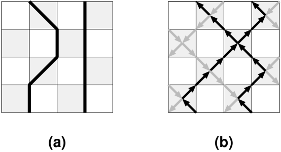
Figure 1: Example of a worldline configuration on a checkerboard lattice of shaded plaquettes. (a) Worldline picture. (b) The same configuration as a vertex picture. Space direction (index $i$) is horizontal, imaginary time direction (index $l$) vertical. The variables $S^{z}_{i,l}$ are defined on each lattice site. Worldlines (arrows upwards in time) denote $S^{z}_{il}=+{1\over 2}$, empty sites (arrows downwards in time) denote $S^{z}_{il}=-{1\over 2}$. The Hamiltonian $\hat{H}_{i,i+1}$ acts on the shaded plaquettes.

The weight $W_{p}$ at each plaquette

$$W_{p}(S_{p})=\langle S^{z}_{i,l}S^{z}_{i+1,l}|e^{-(\Delta\tau)\hat{H}_{i,i+1}}|S^{z}_{i,l+1}S^{z}_{i+1,l+1}\rangle\;,$$ (2.5)

where $\Delta\tau\equiv\beta/L_{t}$, is given by the matrix elements of $\hat{\cal H}=(\Delta\tau){\hat{H}_{i,i+1}}$:

$$\begin{array}[]{lccccccccccc}W(1^{+})&\!\!\equiv\!\!&a_{+}&\!\!\equiv\!\!&\langle{++}|e^{-\hat{\cal H}}|{++}\rangle&\!\!=\!\!&&&e^{-\frac{\Delta\tau}{4}J_{z}}&e^{+\frac{\Delta\tau}{2}h}\\[6.45831pt] W(1^{-})&\!\!\equiv\!\!&a_{-}&\!\!\equiv\!\!&\langle{--}|e^{-\hat{\cal H}}|{--}\rangle&\!\!=\!\!&&&e^{-\frac{\Delta\tau}{4}J_{z}}&e^{-\frac{\Delta\tau}{2}h}\\[6.45831pt] W(2^{\pm})&\!\!\equiv\!\!&c&\!\!\equiv\!\!&\langle{+-}|e^{-\hat{\cal H}}|{+-}\rangle&\!\!=\!\!&\langle{-+}|e^{-\hat{\cal H}}|{-+}\rangle&\!\!=\!\!&e^{+\frac{\Delta\tau}{4}J_{z}}&\cosh{(\frac{\Delta\tau}{2}|J_{x}|)}\\[6.45831pt] W(3^{\pm})&\!\!\equiv\!\!&b&\!\!\equiv\!\!&\langle{+-}|e^{-\hat{\cal H}}|{-+}\rangle&\!\!=\!\!&\langle{-+}|e^{-\hat{\cal H}}|{+-}\rangle&\!\!=\!\!&e^{+\frac{\Delta\tau}{4}J_{z}}&\sinh{(\frac{\Delta\tau}{2}|J_{x}|)}.\end{array}$$ (2.6)

Since $[\hat{H}_{i,i+1},\hat{S}^{z}_{tot}]=0$, there are only the six nonvanishing matrix elements given in eq. (2.6), namely those that conserve $\hat{S}^{z}_{i}+\hat{S}^{z}_{i+1}$, as shown pictorially in figure 3. Therefore, the locations of $S^{z}_{il}=+{1\over 2}$ in figure 1(a) can be connected by continuous worldlines. The worldlines close in imaginary time-direction because of the trace in eq. (2.3).

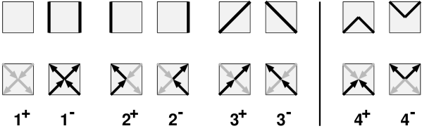
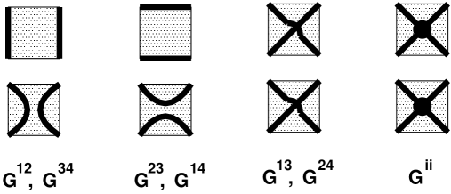
Figure 2: Allowed plaquette configurations $S_{p}$. Top line: worldline picture. Bottom line: the same plaquettes in vertex picture. In the XXZ case (= six-vertex case), only the plaquettes with continuous worldlines, $S_{p}=1^{\pm},2^{\pm},3^{\pm}$, have nonzero weight, eq. (2.6). In the anisotropic XYZ case (= eight-vertex case) the plaquettes $4^{\pm}$ also have nonzero weight.

Figure 3: Graphical representations of plaquette breakups. Top row: worldline picture. Middle row: the same graphs in the vertex picture. A “breakup” specifies the direction in which the two loop segments that enter each plaquette will continue. This direction can be vertical, horizontal, or diagonal. Each graphical representation applies in general to two breakups “$G^{ij}$”, as denoted below the pictures. In the six-vertex-case, breakups $G^{i4}$ do not occur, thus the three non-freezing breakups $G^{ij}$, $i\neq j$ are one-to-one equivalent to the three graphical representations. Breakup “$G^{ij}$” is allowed (i.e. compatible with continuity of the arrow directions of the worldlines ) in plaquette configurations $S_{p}=i^{\pm}$ or $j^{\pm}$ (see figure 3). Namely, flipping the two spins on either one of the two lines in the graphical representation of $G^{ij}$, $i\neq j$, maps between configurations $i$ and $j$. Breakup $G^{ii}$, called “freezing”, forces all four spins to flip together, thus mapping between $i^{+}$ and $i^{-}$. For example, the diagonal breakup $G^{13}$ is compatible with plaquette configurations $1^{\pm}$ and $3^{\pm}$, which is most obvious in the vertex picture. Starting from, e.g., plaquette $1^{-}$ and flipping two diagonally connected spins results in plaquettes $3^{+}$ or $3^{-}$.

For models with fermions or hard core bosons one inserts occupation number eigenstates instead of $S^{z}_{ij}$. Nearest neighbor hopping then again leads to the six-vertex case [5] of figure 3. The term “worldline” derives from this case, since here they connect sites occupied by particles.

We will find it useful to also visualize worldline configurations in a slightly different way, namely as configurations of a vertex model [54]. To do this, we perform a one-to-one mapping of each worldline configuration to a vertex configuration. We stay on the same lattice of shaded plaquettes. We represent each spin $S^{z}_{il}$ by an arrow between the centers of the two shaded plaquettes to which the site $(i,l)$ belongs. The arrow points upwards (downwards) in time for $S^{z}_{il}=+{1\over 2}$$(-{1\over 2})$. The worldline-configuration in figure 1(a) is thus mapped to the vertex configuration of figure 1(b). The one-to-one mapping of the worldline-plaquettes is shown in figure 3. The conservation of $\hat{S}^{z}_{tot}$ on each shaded plaquette means in vertex language that for each vertex (center of shaded plaquette) two arrows point towards the vertex and two arrows point away from it. If one regards the arrows as a vector field, then this means a

condition   “divergence = zero”   for the arrows. (2.7)

Note again that vertex language and worldline language refer to the same configurations; they differ only in the pictures drawn.

We have now mapped the XXZ quantum spin chain to the six-vertex model of statistical mechanics [54], though with unusual boundary conditions, since the vertex lattice here is tilted by 45 degrees with respect to that of the standard six-vertex model. Let us look more closely at the case of vanishing magnetic field, $h=0$. This model has been exactly solved in (1+1) dimensions [54]. The exact phase diagram is shown in figure 4, in terms of the plaquette weights given in eq. (2.6) and in figure 3.

Figure 4: Exact phase diagram of the classical six-vertex model [54] at $h=0$. The weights $a,b,c$ are defined in eq. (2.6). Phase III is massless (infinite correlation length). At $\frac{a}{c}+\frac{b}{c}=1$ there is a Kosterlitz-Thouless phase transition [56] to the massive (finite correlation length) phase IV, and at $\frac{a}{c}-\frac{b}{c}=1$ there is a first order KDP phase transition [57, 58] to the ferroelectric phase I. The parameter regions of the Heisenberg model are denoted in brackets: $J_{z}\geq|J_{x}|$ (AF), $J_{z}\leq-|J_{x}|$ (FM), and $|J_{z}|<|J_{x}|$ (XY-like). The weights corresponding to the XY-model (or free fermions), i.e. $J_{z}=0$, are located on the circle $a^{2}+b^{2}=c^{2}$. When $\Delta\tau\rightarrow 0$, the point $(a/c=1,b/c=0)$ is approached in all cases.

It is interesting to note where the couplings of the Trotter-discretized XXZ-model at $h=0$ are located in this phase diagram (see eq. (2.6)): For the Heisenberg antiferromagnet $J_{z}=|J_{x}|>0$ we have $a+b=c$, i.e. we are on the Kosterlitz-Thouless line. As $\Delta\tau\!\rightarrow\!0$, we approach the point $a/c=1$, $b/c=0$. For the Heisenberg ferromagnet $J_{z}=-|J_{x}|<0$ we have $a-b=c$, i.e. we are on the KDP transition line, approaching the same point $a/c=1$, $b/c=0$ as $\Delta\tau\!\rightarrow\!0$. When $|J_{z}|<|J_{x}|$, the same point is approached from inside the massless (XY-like) region. When $|J_{z}|>|J_{x}|$, it is approached from below the respective transition line, i.e. from the massive (Ising-like) phase IV when $J_{x}>0$ (AF) and from phase I when $J_{x}<0$ (FM). Note that the local couplings $a,b,c$ do not change in higher dimensions (see section 2.12).

Anisotropic XYZ case:  For generality later on, let us briefly describe the anisotropic case without magnetic field, in which $J_{x}\neq J_{y}$ in the Hamiltonian

$$\begin{array}[]{lllllllll}\hat{H}&=\sum_{\langle{\bf ij}\rangle}J_{x}\hat{S}^{x}_{{\bf i}}\hat{S}^{x}_{{\bf j}}\,+\,J_{y}\hat{S}^{y}_{{\bf i}}\hat{S}^{y}_{{\bf j}}\,+\,J_{z}\hat{S}^{z}_{{\bf i}}\hat{S}^{z}_{{\bf j}}\;.\end{array}$$ (2.8)

We also get this case if we quantize the XXZ-model along an axis different from the $z$-axis. The treatment is the same as for the XXZ-model. Again we use $\hat{S}^{z}$ eigenstates to insert complete sets, and arrive at the following nonvanishing matrix elements on the (1+1)-dimensional checkerboard lattice,

$$\begin{array}[]{lccccccccccc}W(1^{\pm})&\!\!\equiv\!\!&a&:=&\langle{++}|e^{-\hat{\cal H}}|{++}\rangle&\!\!=\!\!&\langle{--}|e^{-\hat{\cal H}}|{--}\rangle&\!\!=\!\!&e^{-\frac{\Delta\tau}{4}J_{z}}&\mbox{ch}{(\frac{\Delta\tau}{4}(J_{x}-J_{y}))}\;,\\[6.45831pt] W(2^{\pm})&\!\!\equiv\!\!&c&:=&\langle{+-}|e^{-\hat{\cal H}}|{+-}\rangle&\!\!=\!\!&\langle{-+}|e^{-\hat{\cal H}}|{-+}\rangle&\!\!=\!\!&e^{+\frac{\Delta\tau}{4}J_{z}}&\mbox{ch}{(\frac{\Delta\tau}{4}(J_{x}+J_{y}))}\;,\\[6.45831pt] W(3^{\pm})&\!\!\equiv\!\!&b&:=&\langle{+-}|e^{-\hat{\cal H}}|{-+}\rangle&\!\!=\!\!&\langle{-+}|e^{-\hat{\cal H}}|{+-}\rangle&\!\!=\!\!&e^{+\frac{\Delta\tau}{4}J_{z}}&\mbox{sh}{(-\frac{\Delta\tau}{4}(J_{x}+J_{y}))}\;,\\[6.45831pt] W(4^{\pm})&\!\!\equiv\!\!&d&:=&\langle{++}|e^{-\hat{\cal H}}|{--}\rangle&\!\!=\!\!&\langle{--}|e^{-\hat{\cal H}}|{++}\rangle&\!\!=\!\!&e^{-\frac{\Delta\tau}{4}J_{z}}&\mbox{sh}{(-\frac{\Delta\tau}{4}(J_{x}-J_{y}))}\;,\end{array}$$ (2.9)

which reduce to eq. (2.6) when $J_{x}=J_{y}$. We see that now there is an additional type of vertex with weight $d$, shown as type $4^{\pm}$ in figure 3, in which all four arrows point either towards or away from the center. This vertex type may be thought of as a source (resp. sink) of arrows. Eq. (2.7) becomes the

condition   “divergence = zero mod 4”   for the arrows. (2.10)

The vertices and their weights now correspond to the eight-vertex model [54]. We will see that very little changes for the loop algorithm in this case [3].

2.2 Outline of the Loop Algorithm

The traditional way to perform Monte Carlo updates on a worldline configuration [5, 59] consists of proposing local deformations of worldlines and accepting/rejecting them with suitable probability. In contrast, the updates for the loop algorithm are very nonlocal. We will first describe the basic idea for the example of the XXZ case and outline the resulting procedure. We postpone the formal discussion and the calculation of Monte Carlo probabilities to the next section.An alternative derivation on an operator level is provided in section 3.

Two observations lead to the loop algorithm:

(1) The Hamiltonian acts locally on individual plaquettes. Thus the detailed balance condition on Monte Carlo probabilities can be satisfied locally on those plaquettes.

(2) The allowed configurations of arrows in the six-vertex-case have zero divergence, eq. (2.7). Therefore any two allowed configurations can be mapped into each other by changing the arrow-direction on a set of closed loops, where along each of these loops, the arrows have to point in constant direction. These are the loops that are constructed in our algorithm. The path of the loops will be determined locally on each plaquette (see below).

An example is given in figure 5. Note that the loops are not worldlines; instead they consist of the locations of (proposed) changes in the worldline occupation number (=arrow directions = spin directions). Also, the loops are not prescribed, instead they will be determined stochastically, with probabilities that depend on the current worldline configuration. Since both the zero divergence condition and detailed balance can be satisfied locally at the plaquettes, we will be able to construct the loops by local stochastic decisions on the plaquettes, yet achieve potentially very nonlocal worldline updates.

Let us construct a loop (see figure 5). This is most easily done using the vertex picture, where the loop follows the arrows of the spin-configuration. We start at some arbitrary site $(il)$ of the plaquette lattice and follow the arrow of the current spin configuration into the next plaquette. There we have to specify the direction in which we will continue. For any allowed spin configuration (see figure 3) there are two possibilities to continue along an arrow. We choose one of these directions and follow the arrow into the next plaquette. Then we continue to choose a direction at each of the plaquettes which we traverse. If we reach a plaquette a second time, there is only one direction left to go, since the loop should not overlap itself to avoid undoing previous changes. Eventually we will (on a finite lattice) reach the starting point again, thus closing the loop. If we flip all the arrows (=spins) along the loop, we maintain the continuity of arrows (worldlines) at each plaquette, and thus reach a new valid spin configuration.

We can now start to construct another loop (not to overlap the first one), starting at some other arbitrary site which has not been traversed by the first loop. Note that by deciding the directions in which the first loop travelled, we have at those plaquettes also already determined the direction in which a second loop entering the same plaquettes will move, namely along the two remaining arrows. Thus, what we actually decide at each plaquette through which a loop travels, is a “breakup” of the current arrow configuration into two disconnected parts, denoting the paths that the two loop segments on this plaquette take. The possible breakups of this kind are shown and described in figure 3. For each of the six possible arrow configurations $i^{\pm}$, figure 3, there are two breakups which are compatible with the constraint that the arrows along the loop have to point in a constant direction; namely those breakups labelled $G^{ij},(i\neq j)$ in figure 3.

There is another kind of “breakup” that maintains condition (2.7). Here all 4 spins on a plaquette are forced to be flipped together. We call this choice “freezing” (labeled $G^{ii}$ in figure 3), since for a flip-symmetric model like the six-vertex model at $h=0$ it preserves the current weight $W(i^{\pm})$. Freezing $G^{ii}$ can also be viewed as consisting of either one of the two breakups $G^{ij}$ $(j\neq i)$, with the two loop segments on this plaquette being “glued” together. In this view freezing causes sets of loops to be glued together. We shall call such a set (often a single loop) a “cluster”. All loops in a cluster have to be flipped together. (For an alternative, see section 3.3.)

Overall, we see that by specifying a breakup for every shaded plaquette, the whole vertex configuration is subdivided into a set of clusters which consist of closed loops. Each site of the checkerboard lattice is part of one such loop. We shall call such a division of the vertex configuration into loops a “graph” $G$. Flipping the direction of arrows (= spin or occupancy) on all sites of one or more clusters of a graph (a “cluster flip” which consists of “loop flips”), leads to a new allowed configuration. In the loop algorithm the loops are constructed by specifying breakups with suitable probabilities that depend on the current configuration (see below). In the vertex picture, the graph $G$ resides on the same arrows as the spins. In the worldline picture, the elements of $G$ look slightly differently, as seen in figures 5 and 3 . Note that by introducing loops, we have effectively extended the space of variables, from spins, to spins and breakups. This point will be formalized in the next section.

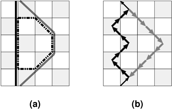
Figure 5: Example of a loop update. (a) Worldline picture. The thick solid line denotes a single worldline, the dot-dashed line depicts a possible loop. By “flipping the loop”, i.e. flipping the spin direction (arrow direction) on all sites along the loop, the worldline will be deformed into the dashed shape. Since the loop can potentially be very large, this deformation can be very nonlocal. (b) The same situation as a vertex picture. The loop is represented by the thick arrows. By construction, in the vertex picture each loop follows arrows of the spin-configuration. This means that the loop runs upwards in time-direction along sites with spin $S^{z}_{il}=+{1\over 2}$, i.e. along worldlines, and downwards in time-direction where there is no worldline.

In summary, the basic procedure for one Monte Carlo update then consists of two stochastic mappings: First from spins to spins plus loops, and then to new spins. I.e., starting with the current configuration of worldlines:

• Select a breakup (i.e. specify in which direction the loops will travel) for each shaded plaquette with a probability that depends on the current spin configuration at that plaquette. These probabilities are discussed below. Identify the clusters which are implicitely constructed by these breakups. This involves a search through the lattice.

• Flip each cluster with suitable probability, where “flipping a cluster” means to change the direction of all arrows along the loops in this cluster (or, equivalently, changing spin direction or occupation number, respectively). The combined cluster flips result in a new spin configuration. The flip probabilities depend in general on the Hamiltonian and on the current spin configuration. In the ideal case, for example the isotropic Heisenberg model in any dimension, each individual loop can be flipped independently with probability $1/2$.

An example is given in figure 6. Notice that in this example the flip of a loop which happened to wind around the lattice in spatial direction led to a change in spatial winding number of the worldline configuration, i.e. an update that cannot be done by local deformations of worldlines.

Figure 6: Example of a worldline update with the loop algorithm. For clarity, we show a situation with only two worldlines. We start with the worldline configuration ${\cal S}$ in the left picture. The stochastic breakup decision on each plaquette, with probabilities depending on this worldline configuration, defines loops (in general clusters of loops), only two of which are drawn. In this example we then flip both loops, i.e. flip the spin direction (= worldline occupancy) along the loops. This results in the new worldline configuration $\SS$ in the right picture, which, as in this example, can be very different from the original one. Since one of the loops happened to wind around the lattice in spatial direction, its flip produced a worldline configuration with nonzero winding number. Note that for the next worldline update, the current loop configuration is discarded, and a completely new set of breakups will be determined with probabilities depending on the new worldline configuration.

Little changes in the general XYZ-like (eight-vertex-like) case [3]. The loops now have to change direction [3] at every breakup of type $(i,4)$. Alternatively, one can also omit assigning a direction to loops.

Let us now cast the general ideas into a valid procedure. Sections 2.3 to 2.6 are formal and comprehensive, with detailed explanations. A summary is given in section 2.6, and explicit weights for XXZ and XYZ cases in section 2.7. A recipe for the most important (yet particularly simple) case, the Heisenberg antiferromagnet, is provided in section 2.8. See also sections 2.13 and 3.6. Previous formal expositions can be found in the original loop algorithm papers [2, 3] (the best formal description there is that for the eight-vertex case in ref. [3]), as well as, in a general setting and in a more suitable language closer to the Fortuin-Kasteleyn mapping of statistical mechanics, in the papers by Kawashima and Gubernatis [9, 34]. We shall use both the worldline picture and the vertex picture of ref. [2, 3], in order to provide a bridge between the existing formulations and to make the simple geometry of the problem as obvious as possible. In section 2.10 we point out that for many models it is possible to sum over all spin variables to obtain a pure loop model. We then cover the continuous time limit. Finally, we introduce improved estimators, the single cluster version, and describe the performance of the loop algorithm.

2.3 Kandel-Domany framework

A brief overview of the basics of Monte Carlo algorithms is given in Appendix A. The derivation [2, 3] of the loop algorithm is similar to that for the Swendsen Wang cluster algorithm in statistical mechanics [15] which uses the Fortuin-Kasteleyn mapping of the Ising model to an extended phase space. (For an excellent review see e.g. ref. [60]). A general formalism for such a mapping was given by Kandel and Domany [61]. Here we use a more suitable language similar to that of the general framework of Kawashima and Gubernatis [9], who made the Fortuin-Kasteleyn-like nature of the mapping obvious.

For future use, we first write down the general scheme, without yet making reference to individual spins, loops, or plaquettes. We start with a set $\{{\cal S}\}$ of configurations ${\cal S}$ and a set $\{G\}$ of graphs $G$, which together constitute the extended phase space. The partition function

$$Z=\sum_{\cal S}W({\cal S})$$ (2.11)

depends only on ${\cal S}$. In addition we now choose a new weight function $W({\cal S},G)$ which must satisfy

$$\begin{array}[]{lllllllll}\sum_{G}W({\cal S},G)&=&W({\cal S})\,,\\ W({\cal S},G)&\geq&0\,.\end{array}$$ (2.12)

Thus we have a Fortuin-Kasteleyn-like [62, 63] representation:

$$Z=\sum_{\cal S}\sum_{G}\,W({\cal S},G)$$ (2.13)

A Monte Carlo update now consists of 2 steps:

• Given a configuration ${\cal S}$ (which implies $W({\cal S})\neq 0$), choose a graph $G$ with probability

  $$p(\,{\cal S}\,\!\rightarrow\!\,({\cal S},G)\,)\;=\;\frac{W({\cal S},G)}{W({\cal S})}\;.$$ (2.14)

• Given ${\cal S}$ and $G$ (this implies $W({\cal S},G)\neq 0$), choose a new configuration $(\SS,G^{\prime})$ with a probability $p\left(\,({\cal S},G)\!\rightarrow\!(\SS,G^{\prime})\,\right)$ that satisfies detailed balance with respect to $W({\cal S},G)$:

  $$W({\cal S},G)\times p\left(\,({\cal S},G)\!\rightarrow\!(\SS,G^{\prime})\,\right)\;=\;W(\SS,G^{\prime})\times p\left(\,(\SS,G^{\prime})\!\rightarrow\!({\cal S},G)\,\right)\;,$$ (2.15)

  for example the heat-bath-like probability

  $$p\left(\,({\cal S},G)\!\rightarrow\!(\SS,G^{\prime})\,\right)\;=\;\frac{W(\SS,G^{\prime})}{W({\cal S},G)+W(\SS,G^{\prime})+\mbox{\em const}}\;.$$ (2.16)

Then the mapping ${\cal S}\!\rightarrow\!\SS$ also satisfies detailed balance with respect to the original weight $W({\cal S})$. Proof:

$$\begin{array}[]{lllllllll}W({\cal S})\,p({\cal S}\!\rightarrow\!{\cal S}^{\prime})&\!\!=\!\!&W({\cal S})&\;\sum_{G,G^{\prime}}\,p(\,{\cal S}\!\rightarrow\!({\cal S},G)\,)\;\;p\left(\,({\cal S},G)\!\rightarrow\!(\SS,G^{\prime})\,\right)\\ &\!\!=\!\!&W({\cal S})&\;\sum_{G,G^{\prime}}\,\frac{W({\cal S},G)}{W({\cal S})}\;\;p\left(\,(\SS,G^{\prime})\!\rightarrow\!({\cal S},G)\,\right)\;\frac{W(\SS,G^{\prime})}{W({\cal S},G)}\\ &\!\!=\!\!&W(\SS)&\;\sum_{G,G^{\prime}}\,\frac{W(\SS,G^{\prime})}{W(\SS)}\;\;p\left(\,(\SS,G^{\prime})\!\rightarrow\!({\cal S},G)\,\right)\\ &\!\!=\!\!&W(\SS)&\;\sum_{G,G^{\prime}}\,p(\,\SS\!\rightarrow\!(\SS,G^{\prime})\,)\;\;p\left(\,(\SS,G^{\prime})\!\rightarrow\!({\cal S},G)\,\right)\\ &\!\!=\!\!&W(\SS)&\;p({\cal S}^{\prime}\!\rightarrow\!{\cal S})\;.\end{array}$$ (2.17)

(Within a Monte Carlo simulation the denominators in eq. (2.17) cannot vanish.)

2.4 Exact mapping of plaquette models

We apply the Kandel-Domany formalism to a model defined on plaquettes, with

$$\begin{array}[]{lllllllll}W({\cal S})&=&A_{global}({\cal S})\,\times\,W^{plaq}({\cal S})\;,\\ &=&A_{global}({\cal S})\,\times\,\prod_{p}W_{p}(S_{p})\;.\end{array}$$ (2.18)

To cover the general case, we have split off a global weight factor $A_{global}$. This split is not unique. We devise an algorithm for $W^{plaq}({\cal S})\equiv\prod_{p}W_{p}(S_{p})$. Because of its product structure, we can perform the decomposition into graphs separately on every plaquette. Thus in analogy with eq. (2.12) we look for a set of “breakups” $G_{p}$ and new weights $W_{p}(S_{p},G_{p})$ on every plaquette $p$ which satisfy

$$\begin{array}[]{lllllllll}\sum_{G_{p}}W_{p}(S_{p},G_{p})&=&W_{p}(S_{p})\,,\\ W_{p}(S_{p},G_{p})&\geq&0\,.\end{array}$$ (2.19)

This implies eq. (2.12) again, both for the plaquette part

$$W^{plaq}({\cal S})=\prod_{p}\,\sum_{G_{p}}\;W_{p}(S_{p},G_{p})=\sum_{\bigcup_{p}G_{p}}\,\prod_{p}\,W_{p}(S_{p},G_{p})\equiv\sum_{G}\,W^{plaq}({\cal S},G)\;$$ (2.20)

(where $G\equiv\bigcup_{p}G_{p}$, $W^{plaq}({\cal S},G)\equiv\prod_{p}\,W_{p}(S_{p},G_{p})$) and for the total weight $W({\cal S})=\sum_{G}W({\cal S},G)$ with

$$\begin{array}[]{lllllllll}W({\cal S},G)&=&A_{global}({\cal S})\times W^{plaq}({\cal S},G)\\ &=&A_{global}({\cal S})\times\prod_{p}W_{p}(S_{p},G_{p})\;.\end{array}$$ (2.21)

Thus we can apply the Kandel-Domany procedure. Restricting ourselves to $G^{\prime}=G$, the two steps i), ii) in the previous section now become the procedure for the loop algorithm. Starting with a configuration ${\cal S}$, a Monte Carlo update consists of:

• Breakup: For each plaquette, satisfy eq. (2.14) by choosing $G_{p}$ with probability

  $$p(\,S_{p}\,\!\rightarrow\!\,(S_{p},G_{p})\,)\;=\;\frac{W_{p}(S_{p},G_{p})}{W_{p}(S_{p})}\;.$$ (2.22)

• Flip: Choose a new configuration $(\SS,G)$ with a probability $p\left(\,({\cal S},G)\!\rightarrow\!(\SS,G)\,\right)$ that satisfies detailed balance with respect to $W({\cal S},G)$.

In the next section we shall explicitely find a suitable set of breakups $G_{p}$ and plaquette weights $W_{p}(S_{p},G_{p})$.

2.5 Structure of plaquette weight functions

Given a graph $G$, we demand that $W^{plaq}({\cal S},G)$ does not change

$$W^{plaq}({\cal S},G)=W^{plaq}(\SS,G)$$ (2.23)

upon any spin update allowed by $W^{plaq}(\SS,G)\neq 0$. Then it cancels in eq. (2.16), which can now be written as

$$p_{flip}({\cal S}\!\rightarrow\!\SS)=\frac{A_{global}(\SS)}{A_{global}({\cal S})+\sum_{\SS\neq{\cal S},W(\SS,G)\neq 0}A_{global}(\SS)}\;.$$ (2.24)

The configurations $\SS$ for which $W(\SS,G)\neq 0$ will be those reached by cluster flips. By enforcing eq. (2.23), all cluster flips will become independent of each other, up to acceptance with $A_{global}$. Eq. (2.23) is equivalent to

$$W^{plaq}({\cal S},G)=\Delta({\cal S},G)\;V(G)\;,\;\;\Delta({\cal S},G):=\left\{\begin{array}[]{lll}1,\;W^{plaq}({\cal S},G)\neq 0,\\ 0,\;\mbox{otherwise}\end{array}\right.\;,$$ (2.25)

which is the form introduced in ref. [9]. Thus

$$W(S,G)=\Delta({\cal S},G)\;V(G)\;A_{global}({\cal S}).$$ (2.26)

We shall achieve eq. (2.23) by enforcing it on every plaquette:

$$W_{p}(S_{p},G_{p})=W_{p}(S_{p}^{\prime},G_{p})\,.$$ (2.27)

Then eq. (2.26) also holds on the plaquette level: $W_{p}(S_{p},G_{p})=\Delta({\cal S}_{p},G_{p})V(G_{p})$. The nontrivial part in this point of view is that all allowed plaquette updates $S_{p}\!\rightarrow\!S_{p}^{\prime}$ match for different plaquettes, to give an overall allowed update ${\cal S}\!\rightarrow\!\SS$. As we have seen in section 2.2, it is the six- (or eight-) vertex constraint, stemming from local conservation of $S^{z}$ (or $S^{z}\mbox{\ \em mod}\ 2)$ in the Hamiltonian, that makes these plaquette updates match in the form of loops. In other words, by enforcing eq. (2.27), we will achieve that all clusters (sets of loops that are glued together at frozen plaquettes) constructed during the breakup-step can be flipped independently, up to acceptance with $p_{flip}$, eq. (2.24).

Let us now find weights satisfying eq. (2.27). Independent cluster flips require that eq. (2.27) at least include the case $S_{p}^{\prime}=\overline{S}_{p}$, where all four spins at a plaquette are flipped, $W_{p}(S_{p},G_{p})=W_{p}(\overline{S}_{p},G_{p})$, which implies the requirement

$$W_{p}(S_{p})\equiv\sum_{G_{p}}W_{p}(S_{p},G_{p})=\sum_{G_{p}}W_{p}(\overline{S}_{p},G_{p})=W_{p}(\overline{S}_{p})$$ (2.28)

on the plaquette weights $W_{p}(S_{p})$. The first step in our construction is therefore to

$$\mbox{\em Choose \ }A_{global}\mbox{\em\ \ such that \ \ }W_{p}(S_{p})=W_{p}(\overline{S}_{p})\;.$$ (2.29)

Such an $A_{global}$ always exists. It is not unique. The ideal case is $A_{global}=\mbox{\em const}$, since then for each cluster, $p_{flip}\equiv\frac{1}{2}$ can be chosen. See also section 4.3.

For worldline models, there are a total of eight allowed spin configurations $S_{p}=i^{\pm}=1^{\pm},2^{\pm},3^{\pm},4^{\pm}$, as shown in figure 3. With eq. (2.28), the plaquette weight $W_{p}(S_{p})$ depends only on $i$. Following ref. [3], let us

$$\mbox{Define a different ``{\bf breakup}'' \ }G_{p}:=G^{ij}\equiv G^{ji}\mbox{\ for every transition \ }i\leftrightarrow j\;,$$ (2.30)

such that the breakup $G^{ij}$ allows exactly the transitions $i\leftrightarrow j$. Thus we define

$$W_{p}(S_{p},G^{ij}):=\left\{\begin{array}[]{llll}w^{ij},&\mbox{if}\;S_{p}=i^{\pm}\;\mbox{or}\;S_{p}=j^{\pm}\;,\\ 0&\mbox{otherwise}\end{array}\right.\;$$ (2.31)

with suitable constants $w^{ij}\equiv w^{ji}$. We have satisfied eq. (2.27) by construction. By inspection of figure 3 we see that every transition $i\leftrightarrow j$, $i\neq j$, corresponds to the flip of 2 spins on a plaquette (all four spins for $i^{+}\leftrightarrow i^{-}$).

We also see by inspection of figure 3 that, given the current worldline configuration $S_{p}=i^{\pm}$, we can identify each of the 4 breakups $G^{ij}$, $j=1,2,3,4$, with one of the graphs in figure 3. Namely, flipping 2 of the spins connected in the graph for $G^{ij}$, $i\neq j$, leads to one of the two plaquette configurations $j^{\pm}$, flipping the other two spins leads to the other configuration, flipping all four spins maps from $i^{\pm}$ to $i^{\mp}$. For an example, see the figure caption. Therefore, given a worldline configuration, the combined breakup $G=\bigcup_{p}G_{p}$ can be representedas a graph consisting of the plaquette-elements in figure 3. In many cases we can also transform the worldline model entirely into a loop graph model; see section 2.10.

Since $G_{p}$ connects pairs of sites, the breakups of all plaquettes will combine to give a set of clusters consisting of loops, as already described in section 2.2. When there is no freezing, i.e. no breakups $G^{ii}$ occur, then all clusters consist of single loops.

We still need to find constants $w^{ij}\equiv w^{ji}$, $i,j=1,2,3,4$, such that the constraint eq. (2.19) is satisfied, which now reads

$$\begin{array}[]{lllllllll}\sum_{j}w^{ij}&=&W(i)\,,\\[6.45831pt] w^{ij}&\geq&0\,,\end{array}$$ (2.32)

(with $W(4)=0$ in the six-vertex-case). This constraint underdetermines the $w^{ij}$. There are 3 equations for 6 unknowns in the six-vertex case, and 4 equations for 10 unknowns in the eight-vertex case. It can always be solved. One explicit solution is the following: Let $W(k)$ be the smallest of the $n$ weights $W(j)$, $j=1,..,n$ ($n$ is $3$ or $4$). Eq. (2.32) is satisfied by

$$\begin{array}[]{lllllllll}w^{ij}=W(k)/n&\;\mbox{for}\;i\neq j\;,\\ w^{ii}=W(i)-\sum_{j\neq i}w^{ij}&\;\mbox{for}\;i=1,..,n\;.\end{array}$$ (2.33)

Experience tells us that for an efficient algorithm, one should keep the loops as independent as possible. Thus we should minimize the weights $w^{ii}$ which cause loops to be glued together. Let $W(l)$ be the largest of the $n$ weights $W(j)$. Given a solution $w^{ij}$ we can always find another one in which no diagonal element $w^{ii}$ except at most $w^{ll}$ is nonzero [34]. For example, to remove $w^{jj},j>1$, define

$$\begin{array}[]{lllllllll}w^{\prime\,j,j}&&=0\\ w^{\prime\,j,j-1}&=w^{\prime\,j-1,j}&=w^{j-1,j}&+&w^{jj}\\ w^{\prime\,j-1,j-1}&&=w^{j-1,j-1}&-&w^{jj}\;.\end{array}$$ (2.34)

Iterating this transformation leads to the one surviving diagonal element

$$w^{\prime\,ll}=w^{ll}-\sum_{i\neq k}w^{ii}\;.$$ (2.35)

More explicit solutions are given in section 2.7.

2.6 Summary of the loop algorithm

Since the detailed derivation of the general formalism was a bit tedious, we summarize the actual procedure here. Start with a model in worldline representation with $Z=\sum_{\cal S}W({\cal S})$, eq. (2.11).

• Choose a split $W({\cal S})=A_{global}({\cal S})\,\times\,\prod_{p}W_{p}(S_{p})$, eq. (2.18), such that $W_{p}(S_{p})=W_{p}(\overline{S}_{p})$, eq. (2.29).

• Find new weights $w^{ij}=w^{ji}\geq 0$ such that $\sum_{j}w^{ij}=W(j)$, eq. (2.32), while preferrably minimizing the “freezing” weights $w^{ii}$, see eq. (2.34). (See also section 3.3).

Each Monte Carlo update from a worldline configuration to a new one then involves the following steps:

• (Breakup) For each shaded plaquettes, with current spin configuration $i^{\pm}$, choose a breakup $G^{ij}$ with probability $p=w^{ij}/W(i)$, proportional to the graph weight $w^{ij}$. (See eqs. (2.22,2.31) and section 2.7).

• (Cluster identification) All plaquette breakups together subdivide the vertex lattice into a set of clusters, which consist of closed loops. Loops which have a frozen vertex (“$G^{ii}$”) in common belong to the same cluster. Identify which sites belong to which clusters. (This is in general the most time consuming task).

• (Flip) Flip each cluster separately, one after the other, with (e.g.) heat-bath probability for $A_{global}$. In case $A_{global}\equiv 1$, this means that one can flip each cluster independently with probability $1\over 2$. “Flipping” means to change the sign of $S^{z}_{il}$ on all sites in the cluster. If desired, one can artificially restrict the simulation to some sector of phase space, e.g. to the “canonical ensemble” of constant magnetization, by prohibiting updates that leave this sector, or one can select such sectors a posterior [64, 65]. (See also section 4.3).

2.7 Graph weights for the XXZ, XYZ, and Heisenberg model

We now come back to our example and compute [2, 3] one solution for the weights $w^{ij}\equiv w^{ji}$, and thus the breakup and flip probabilities, for the spin-flip symmetric six-vertex case, with weights $a$,$b$,$c$, eq. (2.6). This includes the Heisenberg model and the XXZ-model at $h=0$ (eq. (2.6)) in any dimension (see section 2.12). Some solutions for the general XYZ model are also given. We need to find a solution to eq. (2.32). Here it reads

$$\begin{array}[]{lllllllll}w^{11}+w^{12}+w^{13}&=W(1)&\equiv&a&\simeq&1-\frac{\Delta\tau}{2}\,J_{z}\\ w^{22}+w^{12}+w^{23}&=W(2)&\equiv&c&\simeq&1\\ w^{33}+w^{13}+w^{23}&=W(3)&\equiv&b&\simeq&\frac{\Delta\tau}{2}\,|J_{x}|\;.\end{array}$$ (2.36)

From figure 3 we see that $w^{12}$, $w^{23}$, and $w^{13}$ correspond to vertical, horizontal, and diagonal breakups, respectively. The weights $w^{ii}$ correspond to transitions $i^{\pm}\!\rightarrow\!i^{\pm}$, i.e. to flipping zero or four spins on a plaquette. They freeze the value of the weight $W(i)$. Experience tells us that we should minimize freezing in order to get an efficient algorithm, in which then loops are as independent as possible. We will construct solutions with minimal freezing; others exist. See also sections 2.16 and 3.3.

Eq. (2.36) has different types of solutions in different regions of the parameter space $(a,b,c)$. Remarkably, these regions are exactly the same [2, 3] as the phases of the two-dimensional classical six-vertex model [57, 58, 54], shown in figure 4. The regions of figure 4 have been spelled out in terms of the coupling constants $J_{x}$,$J_{z}$ at the end of section 2.1.

Region IV (AF), has antiferromagnetic couplings $J_{z}\geq|J_{x}|$, thus $c\geq a+b$. To minimize the freezing of weight $c$, we have to minimize $w^{22}$. From eq. (2.36), $w^{22}=c-a-b+w^{11}+w^{33}+2w^{13}$. With $w^{ij}\geq 0$ this implies $w^{22,\mbox{\scriptsize min}}=c-a-b$. This minimal value of $w^{22}$ is achieved for $w^{11}=w^{33}=0$, i.e. when we minimize all freezing. The optimized nonzero parameters for region IV are then:

$$\begin{array}[]{lllllllll}w^{12}&=&a&\simeq&1-\frac{\Delta\tau}{2}\,J_{z}&\mbox{(vertical breakup)},\\ w^{23}&=&b&\simeq&\frac{\Delta\tau}{2}\,|J_{x}|&\mbox{(horizontal breakup)},\\ w^{22}&=&c-a-b&\simeq&\frac{\Delta\tau}{2}\,(J_{z}-|J_{x}|)&\mbox{(freezing of opposite spins)},\end{array}$$ (2.37)

without any diagonal breakups. This has to be modified for non-bipartite lattices; see section 2.9. For an alternative to freezing, see section 3.3.

In region I (FM) with ferromagnetic couplings $J_{z}\leq-|J_{x}|$ and $a>b+c$ we get

$$\begin{array}[]{lllllllll}w^{12}&=&c&\simeq&1&\mbox{(vertical breakup)},\\ w^{13}&=&b&\simeq&\frac{\Delta\tau}{2}\,|J_{x}|&\mbox{(diagonal breakup)},\\ w^{11}&=&a-c-b&\simeq&\frac{\Delta\tau}{2}\,(|J_{z}|-|J_{x}|)&\mbox{(freezing of equal spins)},\end{array}$$ (2.38)

without any horizontal breakups. ( This is similar for region II, $b>a+c$, which does not correspond to a quantum model. There we obtain minimal freezing from eq. (2.37) with indices $2$ and $3$ interchanged, and no vertical breakups.)

Region III (XY-like) has $|J_{z}|<|J_{x}|$, and $a,b,c$ $\leq\frac{1}{2}(a+b+c)$. Here we can set all freezing probabilities to zero, obtaining

$$\begin{array}[]{lllllllll}2w^{12}&=&a+c-b&\simeq&2-\frac{\Delta\tau}{2}\,(|J_{x}|+J_{z})&\mbox{(vertical breakup)},\\ 2w^{23}&=&c+b-a&\simeq&\frac{\Delta\tau}{2}\,(|J_{x}|+J_{z})&\mbox{(horizontal breakup)},\\ 2w^{13}&=&b+a-c&\simeq&\frac{\Delta\tau}{2}\,(|J_{x}|-J_{z})&\mbox{(diagonal breakup)}.\end{array}$$ (2.39)

The isotropic Heisenberg model is located on the boundaries of region III. The antiferromagnet $J_{z}=|J_{x}|$ has $c-a-b=0$, thus only vertical ($w^{12}$) and horizontal ($w^{23}$) breakups. The ferromagnet $J_{z}=-|J_{x}|$ obeys $c-a+b=0$ and has only vertical ($w^{12}$) and diagonal ($w^{23}$) breakups. There is no freezing for the isotropic model.

The classical Ising model is reached in the limit $J_{x}/J_{z}=0$, since then $b=0$, so that there is no more hopping and all worldlines are straight. Remarkably, in this limit the loop algorithm becomes [55] the Swendsen-Wang cluster algorithm [15] ! Frozen plaquettes connect the sites of clusters in the Ising model, i.e. they correspond to the “freezing” operation [61] of the efficient Swendsen-Wang method.

The classical BCSOS model is simulated for $a=b$ [1]. When $a=b=\frac{1}{2}c$, the loop algorithm constructs [1] the boundaries of the clusters which the VMR-cluster algorithm [66, 67, 68, 69, 70] for the (1+1)-dimensional BCSOS model produces, i.e. it constructs these clusters more efficiently. The loop representation was used in ref. [71] to obtain exact analytical results for this model, and in ref. [72, 73] to study the roughening transition of the BCSOS model.

General XYZ case: (See also ref. [34] for explicit solutions.) The loop algorithm remains unchanged in the XYZ case (see section 2.2), except that at breakups $G^{i4}$, the arrows flip direction. In each of the four ordered regions of the XYZ model we have $W(m)\geq\sum_{i\neq m}W(i)$ for one $m\in\{1,2,3,4\}$. The nonzero breakup weights with minimum freezing are then

$$\begin{array}[]{lllllllll}w^{mm}&=&W(m)-\sum_{i\neq m}W(i)\\ w^{im}&=&W(i)\;\;(i\neq m).\end{array}$$ (2.40)

This also summarizes the solutions for regions I,II,IV above. In the disordered region $2W(m)<\sum_{i}W(i)$ we can set all freezing $w^{ii}$ to zero, and in general still have 6 free parameters $w^{ij}$ with only 4 constraints eq. (2.32).

2.8 Recipe for the spin ${1\over 2}$ Heisenberg antiferromagnet

In order to make the loop algorithm as clear as possible, we restate the procedure for the important yet simple case of the isotropic spin ${1\over 2}$ Heisenberg antiferromagnet. See also section 2.13, for the continuous time version, and section 3.6 for the SSE variant.

A Monte Carlo update leads from a worldline configuration ${\cal S}$ of spin variables $S^{z}_{il}=\pm 1$ to a new configuration ${\cal S}^{\prime}$. On each shaded plaquette $p$, the local spin configuration $S_{p}$ takes one of the six possibilities shown in the left part of figure 3, with weights $W_{p}(S_{p})$ given in eq. (2.6), satisfying $a+b=c$ in the isotropic antiferromagnetic case. The weights $w^{ij}$ in eq. (2.37) are all zero except for $w^{12}=a\,,w^{23}=b$, so that we get only vertical ($G^{12}$) and horizontal ($G^{23}$) breakups. The update consists of the following steps:

• For each shaded plaquette, choose the horizontal breakup with probability

  $$\begin{array}[]{lllllllll}p(S_{p},G^{23})&=&(\delta_{S_{p},2^{\pm}}+\delta_{S_{p},3^{\pm}})\;\;{\frac{w^{23}}{W_{p}(S_{p})}}&=&\left\{\begin{array}[]{lllll}0,&\;S_{p}=1^{\pm}\;,\\ \tanh(\frac{\Delta\tau}{2}J)&\;S_{p}=2^{\pm}\;,\\ 1,&\;S_{p}=3^{\pm}\;,\end{array}\right.\end{array}$$ (2.41)

  (see eqs. (2.6,2.22,2.31,2.37)), otherwise choose the vertical breakup.

• Identify the clusters constructed in step (i). Since there is no freezing here, all clusters consist of single loops.

• Flip each loop with probability $1\over 2$, where flipping means to change the sign of $S^{z}_{il}$ on all sites along the loop. This gives the new configuration ${\cal S}^{\prime}$.

This procedure is even simpler than local worldline updates. Moreover, it remains completely unchanged in arbitrary dimensions (see section 2.12). The single cluster version is described in section 2.11. Note that one can and should avoid the Trotter approximation altogether, by working directly in continuous time, for which a modification of this recipe will be given in section 2.13. or by using the stochastic series expansion, described in section 3.6.

2.9 Ergodicity

To establish correctness of the loop algorithm, we still have to show ergodicity for the overall algorithm, including the existence of global configuration changes, Ergodicity is obvious when all $w^{ij}>0$ for $i\neq j$, and when $p_{flip}$ is always nonzero (which is normally the case when we use eq. (2.24) for $p_{flip}$). Any two allowed configurations (i.e. $W({\cal S})\neq 0$) are, as always, mapped into each other by a unique set of spin-flips (loop-flips), which are compatible with a set of breakups $G^{ij}$, $i\neq j$. With $w^{ij}>0$, this set of breakups has a finite probability to occur, and with $p_{flip}>0$, the two configurations will be mapped into each other in a single Monte Carlo step with finite probability. Note that the trivially ergodic case $w^{ij}>0$ can always be constructed, as seen in eq. (2.33); this may not be an efficient algorithm, however. On the other hand, one can always construct weights $w^{ij}$ such that (for $J_{xy}\neq 0$) ergodicity is not achieved, for example by choosing $w^{ij}=\delta_{ij}W(i)$, i.e. only freezing.

When some of the $w^{ij}$ vanish, ergodicity has to be shown case by case. With the weight choices of section 2.7, region III is trivially ergodic. We have to show ergodicity explicitely in each of the regions I, II, IV, because some $w^{ij}$ vanish there.

Region I (including the Heisenberg FM): $w^{23}=0$, i.e. there are only vertical and diagonal breakups (see figure 3). These breakups permit a loop configuration which is identical to any given worldline configuration. That loop configuration will occur with finite probability. Flipping all loops in this configuration leads to the empty worldline configuration. Conversely, any worldline configuration can be generated from the empty one in a single (!) update by such a choice of loops. Therefore the algorithm is ergodic, mapping any two worldline configurations into each other in only two steps.

Region IV (including the Heisenberg AF): $w^{13}=0$, i.e. there are only vertical and horizontal breakups. On a bipartite lattice with open or periodic spatial boundary conditions, ergodicity can be shown easily. Start with any worldline configuration ${\cal S}=\{S_{xl}\}$. Our reference configuration this time is not the “empty” configuration $S^{\prime}_{xl}=-{1\over 2}$, but instead the staggered configuration $S^{\prime}_{xl}=(-1)^{x}(-{1\over 2})$, i.e. the configuration with straight worldlines on one of the two sublattices. As always, there is a unique set of loops whose flips will map ${\cal S}$ into $\SS$. By inspection we see that these loops contain only vertical and horizontal breakups (horizontal where $\SS$ has diagonal worldline parts, vertical elsewhere). Since these breakups have finite probability to occur, the whole set of loops will be constructed with finite probability. Thus, again, any worldline configuration will be mapped to the reference configuration with finite probability, and vice versa, so that on a bipartite lattice the algorithm is ergodic. Furthermore, on any lattice, the loop algorithm is at least as ergodic as the algorithm with conventional local updates. The latter consist of spin-changes around non-shaded plaquettes, equivalent to the flip of a small loop with two vertical and two horizontal breakups, which will occur with finite probability in the loop algorithm.

Note that for a frustrated antiferromagnet, i.e.  on a non-bipartite lattice, the algorithm eq. (2.37) with only horizontal breakups is not ergodic [42]: Loops switch time-direction at every breakup, thus a loop with an odd number of spatial hops is not possible. To ensure ergodicity, one has to include diagonal breakups with some weight $0<w^{13}<b$. Then ergodicity is trivial, since all $w^{ij}>0$ for $i\neq j$. Eq. (2.36) is now solved with $w^{23}=b-w^{13}$ and demands freezing $w^{22}=2w^{13}$ of equal spins. The size of $w^{13}$ has to be chosen for optimal performance of the algorithm, which, however, is subject to a severe sign problem.

For completeness, we mention region II (which does not occur in worldline models). Here there is no vertical breakup. In case of periodic spatial boundary conditions, interchange of “space” and “time” leads us to the situation of region I, for which we have already shown ergodicity.

2.10 Transformation to a pure loop model

Remarkably, by using the exact mapping eqs. (2.12,2.19) on which the loop algorithm is based, we can transform quantum spin and particle models into pure loop representations, i.e. into a completely different setting than the original worldlines. This is analoguous to the Fortuin-Kasteleyn representation [62, 63] of the Potts model. It was first achieved, independently, by Nachtergaele and Aizenman [10, 11] for the one-dimensional Heisenberg model, and was used to prove rigorous correlation inequalities [10]. Kondev and Henley used it to compute the exact stiffness and critical exponents of a twodimensional vertex model [71, 74]. See also section 3.

We get to a loop model by explicitely summing over the spin degrees of freedom in eq. (2.13). Using eqs. (2.13,2.21,2.25) we see that

$$Z=\;\;\sum_{\{{\cal S}\}}W({\cal S})\;\;=\;\;\sum_{\{{\cal S}\}}\prod_{p}\sum_{G_{p}}\;\Delta(S_{p},G_{p})\;V(G_{p})\;A_{global}({\cal S})\;.$$ (2.42)

The condition $\Delta(S_{p},G_{p})\neq 0$ restricts the graph $G$ to consist of clusters, i.e. divergence-free components compatible with the spin configuration.

The summation over spin configurations ${\cal S}$ can easily be done if a reference spin configuration ${\cal S}_{0}$ exists (see also section 2.9), in which all plaquette breakups $G_{p}$ with nonvanishing weight $V(G_{p})$ are allowed (i.e. $W_{p}(S_{p0},G_{p})>0$ whenever $V(G_{p})>0$). Then all graphs with finite weight can be constructed from $S_{0}$. By design, cluster flips do not change $W(S,G)$ when $A_{global}(S)$ is constant. Each cluster can then be flipped independently and contributes a factor $2$. With the weight choices from section 2.7, we see that for the AF region IV, the antiferromagnetically staggered configuration is such a reference configuration on bipartite lattices: it allows all relevant breakups (vertical, horizontal, freezing of unequal spins) on any plaquette. For region I (FM), the ferromagnetic spin configuration serves the same purpose on any lattice.

In these regions (as well as in region II), we can then sum over spin configurations in eq. (2.42). Without external weight $A_{global}$, we get

$$Z=\;\sum_{G=\bigcup_{p}G^{ij}}\left(\prod_{p}w^{ij}\right)\,2^{N_{c}(G)}\;\;\equiv\;\;\sum_{G}W(G)\;,$$ (2.43)

where $N_{c}(G)$ is the number of clusters in $G$. When $A_{global}$ is a product over contributions from each cluster (e.g. in case of a magnetic field), the factor $2$ for each cluster is replaced by $(A_{global}({\cal S}(G))+A_{global}(\SS(G)))$.

When there is no reference configuration, e.g. for region III (XY-like) or for antiferromagnets on non-bipartite lattices, or for different choices of breakup-weights, we can still obtain a pure loop model. Now there can be clusters which do not correspond to a continuous worldline configuration (i.e. the spin directions mandated by independently chosen breakups at different plaquettes within a cluster may contradict each other). To remove graphs containing such clusters, we temporarily endow each loop with a direction, and introduce a constraint into the sum over graphs in eq. (2.43) enforcing compatibility of the loop directions of each cluster.

The mapping generalizes immediately to the anisotropic XYZ-like case, where the number of a priori breakup-possibilities per plaquette doubles, though they are graphically still the same as in the XXZ-like case (see figure 3).

We have thus mapped all XYZ-like quantum spin and particle models, with any choice of breakup weights and in any dimension, to a loop model, in complete analogy with the Fortuin-Kasteleyn mapping [62, 63] of statistical mechanics. This mapping is useful for analytical purposes (see above). Note that for the Heisenberg antiferromagnet, the loop model consists of antiferromagnetic selfavoiding polygons, and for the Heisenberg ferromagnet it has a similar graphical representations as the worldlines themselves. Note also that for a given physical model there are many different loop models, corresponding to the different possible choices of breakup-weights. Remarkably, the graph-decomposition eq. (2.19), and thus the transformation to a loop model, can also be written on an operator level [12] (see section 4.6). All observables can be measured in the loop representation [12], as correlation functions (“improved estimators”, see sections 2.14, 4.6) or as thermodynamic derivatives.

One can perform Monte Carlo simulations purely in the loop representation, analoguously to Sweeny’s method for the cluster representation of the Ising model [75]. Indeed, closer inspection reveals that the Handscomb method for the ferromagnet is equivalent to a Monte Carlo in loop representation with stochastic series expansion [76, 77, 78, 79, 80, 81] ! For other models this has not yet been tried (but the method of section 4.8 comes close). In more than one spatial dimension, it is computationally more difficult than the loop algorithm with graphs and spins, since one has to keep track of the number of clusters, which can require traversing complete clusters for each local update, unless it can be simplified by a binary tree search.

2.11 Single-Cluster Variant

As in Swendsen-Wang Cluster updates, there are several ways to perform an update of the worldline configuration ${\cal S}$ with the required detailed balance with respect to $W({\cal S},G)$, eq. (2.15). There are two important approaches:

• Multi-Cluster Variant: Determine the whole graph (set of loops) $G$ and flip each cluster (set of mutually glued loops) in $G$ with suitable probability (see section 2.6)

• Single-Cluster Variant (Wolff-cluster) [82, 1] Pick a site $(i_{0},l_{0})$ at random, and construct only the cluster which includes that site. This can be done iteratively, by following the course of the loop through $(i_{0},l_{0})$ until it closes, while determining the breakups (and thus the route of the loop(s)) only on the plaquettes which are traversed. This corresponds to our initial loop-description in section 2.2. At each plaquette at which a frozen breakup $G^{ii}$ is chosen, the current loop is glued to the other loop traversing this plaquette. That other loop (and any loops glued to it) then also has to be constructed completely. Flip the complete cluster with probability $p_{flip}$ satisfying detailed balance with respect to $A_{global}$ to get to a new spin configuration. Note that when $A_{global}=\mbox{\em const}$, we can choose $p_{flip}=1$ instead of $1\over 2$.

Both approaches satisfy detailed balance in eq. (2.15). One may think of the single-cluster variant as if all clusters had actually been constructed first, and then one of them chosen at random, by picking a site, to make an update proposal.

The advantage of the single-cluster variant [82, 83, 60] is that by picking a random site, one is likely to pick a large cluster, whose flip will produce a big change in the configuration and thus a large step in phase space. This can reduce critical slowing down still further. The effort (computer time) to construct the single-cluster is proportional to its length. Normalized to constant effort, one finds indeed that the single-cluster variant (and the corresponding “Wolff-algorithm” for Swendsen-Wang-like algorithms) usually have even smaller dynamical critical exponents (see appendix B) than the multi-cluster variant. Note that improved estimators get a different normalization in the single-cluster variant (see eq. (2.56) and below). In some circumstances, the multi-cluster variant can still be advantageous overall, for example when employing parallel [84, 85, 86] or vectorized [87] computers. It is also essential for the meron method (section 4.8) and e.g. four-point functions as improved estimators (section 4.6), and it is easier to implement in continuous time.

The single-cluster method, on the other hand, generalizes into the worm and directed-loop methods discussed in section 5, which are applicable to any discrete model.

2.12 Arbitrary spatial dimension

There is vitually no change algorithmically in going to higher dimensions [1], if one chooses to stay on a vertex-lattice. Let us look at two spatial dimensions as an example. The even/odd split of the Hamiltonian in eq. (2.2) can be generalized to

$$\hat{H}=\sum_{\nu}\hat{H}_{\nu}=\sum_{\nu}\sum_{i}\hat{H}_{i,i+\hat{\nu}}$$ (2.44)

with a separate $\hat{H}_{\nu}$ for each direction of hopping (resp. spin coupling) in the Hamiltonian $\hat{H}$. For a two-dimensional square lattice with nearest neighbor hopping we thus get 4 parts $\hat{H}_{\nu}$, each the sum of commuting pieces living on single bonds, in complete analogy with the one-dimensional case.

After the Trotter-Suzuki breakup, eq. (2.3), these single bonds again develop into shaded plaquettes. Each Trotter timeslice now has 4 subslices. Locally on each shaded plaquette we have the identical situation as in (1+1) dimension. Thus the loop algorithm can be applied unchanged. The only thing that changes is the way that different plaquettes connect. (Thus it is easy to write a loop-cluster program for general dimension. This contrasts with the traditional local worldline updates, where a number of different rather complicated updates are necessary [88] to achieve acceptable performance). The same construction can be applied as long as the lattice and the Hamiltonian admit a worldline representation in which commuting pieces of the Hamiltonian live on bonds.

2.13 Continuous time

As one of the most important developments, Beard and Wiese [16] have shown that within the loop formulation, one can directly take the time continuum limit $\Delta\tau\!\rightarrow\!0$ in the Trotter-Suzuki decomposition, eq. (2.3). In fact, it turns out that one can also write the original spin model in operator language, directly in continuous time when $H$ has a countable basis (see section 3) [89, 90, 10].

In continuous time it is appropriate to describe worldlines by specifying the times $t$ at which a worldline jumps to a different site. This jump is now instantaneous.

Figure 7: Loop construction in continuous time. Thick solid lines denote worldlines; the thick dashed line is a partial loop.

Let us look again at the simple case of a spin $1\over 2$ antiferromagnet. Figure 7 shows part of a worldline configuration. In discrete time, this picture would be subdivided into plaquettes of temporal extent $\Delta\tau$, like figure 1. On each such plaquette, the probability of a horizontal breakup is given by eq. (2.41)

$$\begin{array}[]{lllllllll}p(\mbox{horiz.\ breakup})&=&\left\{\begin{array}[]{lllll}0,&\;\mbox{0 or 2 worldlines on plaquette}\;,\\ \tanh(\frac{\Delta\tau}{2}J)&\;\mbox{1 straight worldline}\;,\\ 1,&\;\mbox{worldline jumps }\;,\end{array}\right.\end{array}$$ (2.45)

Now look at a specific lattice bond, e.g. $\langle jk\rangle$ in figure 7. For any time interval in which the plaquette occupation on this bond does not change, the breakup probability is constant. Then the breakup probability per time has a continuous time limit, i.e. it becomes a constant probability density. For lattice bond $\langle jk\rangle$ in figure 7 this is for example the case between times $t_{1}$ and $t_{2}$:

$$\frac{p(\mbox{horiz.\ breakup})}{\Delta\tau}~{}~{}~{}~{}~{}\stackrel{{\scriptstyle\Delta\tau\!\rightarrow\!0}}{{\longrightarrow}}~{}~{}~{}~{}~{}\frac{J}{2}$$

Between times $t_{2}$ and $t_{3}$, the probability for a horizontal breakup on this lattice bond from eq. (2.45) is zero. On plaquettes without horizontal breakup, there is a vertical one, which means that loops will just continue in imaginary time without a jump. A third case occurs on lattice bond $\langle ij\rangle$ at time $t_{3}$. Here the probability for a horizontal breakup from eq. (2.45) is 1.

The same pattern holds for the general case: All breakup probabilities on plaquettes are either 0, 1, or proportional to $\Delta\tau$ (for small $\Delta\tau$), and thus have a continuous-time limit. Note that the probability densities are generated by the order $\Delta\tau$ of plaquette weights. Thus they contain matrix elements of the Hamiltonian (or parts of it), and no longer the exponential of $\hat{\cal{H}}$.

The multi-loop algorithm, summarized in section 2.6, therefore obtains a modified breakup-step in continuous time. For each lattice bond:

• Identify each region of imaginary time in which the worldline configuration on this bond does not change. Randomly assign horizontal or diagonal breakups there with constant probability density, given by the continuous time limit of eq. (2.22).

• At times $t$ where a worldline jumps across the lattice bond, there will be a non-vertical breakup with probability one. For example, in case of the Heisenberg antiferromagnet, this will always be a horizontal breakup. In case of the XY-model, eq. (2.39) implies probabilty  $1\over 2$ for both horizontal and diagonal breakups.

The rest of the algorithm remains unchanged. The technical implementation does however change completely. In continuous time, one can no longer store plaquette configurations. Instead, worldlines are specified by the events at which a worldline jumps to a neighboring site. It is useful to store a doubly linked list of such events for each site, with each list-item containing pointers to the preceeding and to the following event on the same site, and a specification of the nature of the event including its time $t$. (For the isotropic ferromagnet one needs only a singly linked list since all movement is forward in imaginary time). The breakup step can then be performed for each lattice bond, by following the lists for the corresponding two sites. Breakups can, e.g., be inserted as a different kind of event into the same lists, or be stored in separate lists. Identification and flipping of clusters then involves manipulations of these linked lists.

The single-loop variant (section 2.11) can also be performed in continuous time. Instead of deciding breakups bond by bond, we now follow an individual loop-end along sites.

Choose a site $j$ at random. Start a loop at an arbitrary time $t_{1}$, moving (e.g.) upwards in time. An example is shown in figure 7. The loop construction iterates the following procedure:

Determine the time interval $t_{1}<t<t_{2}$ (equations are specified for moving upwards in time) during which the worldline occupation of the neighboring sites does not change. Technically this can be implemented by using linked lists of events as above, and including additional pointers for each event, e.g. to preceding events on neighboring sites. For each such neighbor $k$ draw a random number $\tau_{jk}$ from the distribution $\lambda_{jk}\exp{(-\lambda_{jk}\tau_{jk})}$, where $\lambda_{jk}=J_{jk}/2$ is the corresponding breakup probability density. Now move the loop-end on site $j$ up to time $t_{1}+\min_{k}{(\tau_{jk})}$ and let it jump to the corresponding site $k$ there .The situation is the same as in radioactive decay, with decay constants $\lambda_{jk}$ and neighboring sites corresponding to decay channels.

Moving in time-direction on site $i$ corresponds to choosing a vertical breakup for all infinitesimal “plaquettes” connecting site $i$ to its neighbors. When $J_{jk}$ corresponds to a horizontal breakup, the loop-end will move in the opposite time-direction at the new site. When $J_{jk}$ corresponds to freezing, the loop branches and becomes a cluster of loops, as usual.

In the standard loop-algorithm, loops are non-self-overlapping and correspond to those of the pure loop-representation of the simulated model (sections 2.10 and 3). Thus in the above construction one has to exclude those temporal regions of neighboring sites which have already been visited by the single loop (resp. cluster). This constraint is removed for the so-called directed loops, section 5.3.

In case that all transition times $t_{1}+\tau_{jk}$ exceed $t_{2}$, the loop-end stays at site $j$ and moves to time $t_{2}$. If the worldline at site $j$ jumps at time $t_{2}$, the loop must also jump, with the same probabilities as in the discrete time formulation.

Now iterate this procedure. Eventually the loop closes and can be flipped as usual.

We see that in continuous time, the single loop method is technically more involved than the multi-loop algorithm. It also lacks some of the improved estimators of the multi-loop method (see sections 4.6,4.8). On the other hand it tends to have still better autocorrelations. It can also be generalized to the directed-loop method (section 5.3).

The continuous time limit has several important advantages over the discrete time case. It removes completely the systematic error from the Trotter breakup, thus also removing the cumbersome need for calculations at several values of $\Delta\tau$ in order to extrapolate to $\Delta\tau=0$. In addition, worldlines are specified much more economically by just specifying their transition times. This helps especially at low temperatures, by strongly reducing the storage requirements for a simulation. Longer range couplings imply larger sets of neighbors $j$ to treat at each step. This is still cumbersome, but more economical than introducing extra Trotter slices. The advantages of the loop algorithm are preserved.

Other approaches which work without Trotter approximation are the worm algorithm (section 5.1) and the stochastic series expansion (SSE) (sections 3.5,5.2, as well as directed loops (section 5.3).

2.14 Improved Estimators

In addition to the reduction of autocorrelations, the combined representation eq. (2.13) allows a potentially drastic reduction of statistical errors by using so-called improved estimators [82, 83, 91, 46, 42, 75]. The Monte Carlo procedure provides us with a series of configurations ${\cal S}_{i}$. For each such configuration, we construct a graph, with some $n_{i}$ clusters. We can then reach any state in a set ${{\cal F}}_{i}$ of $2^{n_{i}}$ worldline configurations by flipping a subset of the clusters. The probability for each of these configurations is determined by the cluster flip probabilities $p_{flip}$. In the loop algorithm one configuration ${\cal S}_{i+1}$ will be chosen randomly according to these probabilities as the next Monte Carlo configuration. The standard thermal expectation value of an observable $\cal O$ is calculated by averaging over the value of the observable in the configurations ${\cal S}_{i}$:

$$\langle{\cal O}\rangle=\sum_{i}{\cal O}({\cal S}_{i}).$$ (2.46)

An improved estimator with $\langle{\cal O}\rangle=\langle{\cal O}_{impr}\rangle$ can formally be defined as a weighted average of ${\cal O}$ over the states $\SS$ that can be reached from ${\cal S}$ with any valid Monte Carlo procedure. With the loop algorithm we sum over the $2^{n_{i}}$ states $\SS\in{{\cal F}}_{i}$. Since this is a sum over many states, it has reduced variance. Ideally, it can be calculated completely and then depends only on the graph $G$

$${\cal O}_{impr}(G)\;=\;\frac{\sum_{\SS}W(\SS,G){\cal O}(\SS)}{\sum_{\SS}W(\SS,G)}\;=\;\frac{\sum_{\SS\in{{\cal F}}_{i}}A_{global}(\SS){\cal O}(\SS)}{\sum_{\SS\in{{\cal F}}_{i}}A_{global}(\SS)},$$ (2.47)

where we have used eq. (2.26). Note that ${\cal O}_{impr}(G)$ is the representation of $\hat{O}$ in the pure loop model (see sections 2.10, 4.6). Alternatively, the sum in eq. (2.47) can be evaluated stochastically,

$${\cal O}_{impr}({\cal S},G)\;=\;\sum_{\SS\in{{\cal F}}_{i}}\;p_{G}({\cal S}\rightarrow\SS)\;{\cal O}(\SS)\;,$$ (2.48)

where $p_{G}({\cal S}\rightarrow\SS)$ is any probability that satisfies detailed balance for $A_{global}$ (and thus for $W(S,G)$); it need not be equal to the actual update probability. Usually it is a product over suitably chosen cluster flip probabilities $p_{flip}$. We need to calculate this average over $2^{n_{i}}$ states in a time comparable to the time needed for a single measurement. Fortunately that is often possible.

Especially simple improved estimators can be found in the case that $p_{\rm flip}={{1\over 2}}$ for all clusters. Then eq. (2.48) simplifies to

$${\cal O}_{impr}\;=\;2^{-n_{i}}\sum_{\SS\in{{\cal F}}_{i}}{\cal O}(\SS),$$ (2.49)

since all of the states in ${{\cal F}}_{i}$ now have the same probability $2^{-n_{i}}$. In order to achieve $p_{flip}=\frac{1}{2}$ when there is a nontrivial global weight $A_{global}$, we can use a probability function $p_{G}({\cal S}\rightarrow\SS)$ that has some clusters fixed in a certain state, and then has a new flip probability of $1\over 2$  for all other clusters. There are many possibilities. One can for example fix a cluster in its present state with Metropolis probability, or one can [42] fix the state of a cluster with probability $p_{\rm fix}=|2p_{\rm flip}-1|$, in its present state if $p_{\rm flip}<{{1\over 2}}$, and in its flipped stated otherwise. The improved estimators then contain the usual contributions from both states of the non-fixed clusters, as well as contributions from the constant state of the fixed clusters [42]. In the following we assume for simplicity that no clusters are fixed.

Let us calculate some useful improved estimators. Consider as an example the spin correlation function $\langle\hat{S}^{z}_{j}\hat{S}^{z}_{k}\rangle$ between two spins at spacetime sites $j=({\bf r},\tau)$ and $k=({\bf r^{\prime}},\tau^{\prime})$. Since each spin can be in one cluster only, the improved estimator eq. (2.49) is

$$4(\hat{S}^{z}_{j}\hat{S}^{z}_{k})_{impr}=\left\{\begin{array}[]{lll}\sigma_{j}\sigma_{k},&\mbox{\ \ if $j$ and $k$ are in the same cluster},\\ (1-2p_{\rm flip,j})\,(1-2p_{\rm flip,k})\;\sigma_{j}\sigma_{k},&\mbox{\ \ otherwise},\\ \end{array}\right.$$ (2.50)

where $\sigma_{j,k}=\pm 1$ are the current values of the worldline variables ($+1$ for a worldline, $-1$ for an empty site). In case $p_{\rm flip}={{1\over 2}}$, the improved estimator is extremely simple:

$$4(\hat{S}^{z}_{j}\hat{S}^{z}_{k})_{impr}=\left\{\begin{array}[]{lll}\sigma_{j}\sigma_{k},&\mbox{\ \ if sites $j$ and $k$ are in the same cluster},\\ 0,&\mbox{\ \ otherwise.}\end{array}\right.$$ (2.51)

We see that the calculation of improved estimators of correlation functions requires even less effort than for non-improved estimators. Remarkably, the spin-spin correlation function corresponds to the size distribution of the clusters. In general one can compute $n$-point Greens functions, including off-diagonal ones, as improved estimators from the geometric properties of the clusters (section 4.6). Note that for uniform correlations of the the Heisenberg FM and for staggered correlations of the Heisenberg AF, we always have $\sigma_{j}\sigma_{k}=+1$ in eq. (2.51).

The potential gain from using the improved estimator is easy to see when $\sigma_{j}\sigma_{k}=1$. The expectation value is the same as for the unimproved estimator $\sigma_{j}\sigma_{k}=\pm 1$. When $\langle{\cal O}\rangle$ is small (e.g. $\langle{\cal O}\rangle\sim\exp{(-R/\xi)}$ at large distance $R=|{\bf r}-{\bf r^{\prime}}|$), then the variance of ${\cal O}$ is

$$\langle{\cal O}^{2}\rangle-\langle{\cal O}\rangle^{2}\,=\,1-\langle{\cal O}\rangle^{2}\,\approx\,1\;,$$ (2.52)

whereas the variance of ${\cal O}_{impr}$ is

$$\langle{\cal O}_{impr}^{2}\rangle-\langle{\cal O}_{impr}\rangle^{2}\,=\,\langle{\cal O}_{impr}\rangle-\langle{\cal O}_{impr}\rangle^{2}\,\approx\,\langle{\cal O}_{impr}\rangle\equiv\langle{\cal O}\rangle\ll 1\;.$$ (2.53)

For a given distance R, this gain is largest at small correlation length $\xi$, whereas the gain from reducing autocorrelations with the loop algorithm is largest at large $\xi$. On the other hand the non-improved estimator can have a sizeable amount of self-averaging at small $\xi$, so that the gain from using improved estimators as just a measurement tool can be moderate in practice. See, however, sections 4.6 and 4.8 for other drastic effects of using improved estimators.

Especially simple estimators can also be derived for magnetic susceptibilities. The uniform magnetic susceptibility at vanishing magnetic field can be expressed as the sum over all correlation functions:

$$\langle\chi\rangle=\frac{\beta}{V}\left\langle\left(\sum_{\bf r}{1\over M}\sum_{\tau}S^{z}_{{\bf r},\tau}\right)^{2}\right\rangle,$$ (2.54)

where $V$ is the spatial volume (number of sites), $M=2dL_{t}$ is the number of time slices in $d$ dimensions, and $S^{z}_{{\bf r},\tau}=\pm{1\over 2}$. This simplifies [46] in the XXZ case, by using

$$\sum_{\tau}\frac{1}{M}\sum_{\bf r}S^{z}_{{\bf r},\tau}\,=\,\sum_{\mbox{\scriptsize(clusters c)}}\sum_{(({\bf r},\tau)\mbox{\scriptsize in }c)}\frac{1}{M}S^{z}_{{\bf r},\tau}\,=\,{1\over 2}\,\sum_{\mbox{\scriptsize clusters c}}w_{t}(c)$$ (2.55)

to the sum of the square of the temporal winding numbers $w_{t}(c)$ of the clusters $c$:

$$\langle\chi\rangle=\frac{\beta}{4V}\left\langle\sum_{\mbox{\scriptsize clusters c}}w_{t}(c)^{2}\right\rangle$$ (2.56)

In the single-cluster variant (section 2.11), the sum over the clusters in eq. 2.56 is also calculated stochastically. Since we pick a single cluster with a probability $\frac{|c|}{MV}$, where $|c|$ is the cluster size and $MV$ is the number of sites in the space-time lattice, we have to compensate for this extra factor and obtain $\langle\chi\rangle=\frac{\beta}{4V}\left\langle\frac{MV}{|c|}\,w_{t}(c)^{2}\right\rangle$. Similarly, eq. (2.51) implies that for an antiferromagnet with only horizontal breakups, the staggered susceptibility corresponds to the sum over the squares of all cluster sizes,

$$\langle\chi_{s}\rangle=\frac{\beta}{V}\left\langle\left(\sum_{\bf r}(-1)^{\bf r}{1\over M}\sum_{\tau}S^{z}_{{\bf r},\tau}\right)^{2}\right\rangle\;=\;\frac{\beta}{4VM^{2}}\left\langle\sum_{\mbox{\scriptsize clusters c}}|c|^{2}\right\rangle.$$ (2.57)

Further improved estimators can be constructed, including cases with a sign problem [42]. Moreover, it was discovered [20] that by clever use of the improved estimator for the fermion sign, one can perform fermionic simulations in a restricted class of models without sign problem; see section 4.8.

2.15 Infinite Lattices and Zero Temperature

The existence of a single cluster version (section 2.11) and of improved estimators for two-point functions which have support only on individual clusters, allows for a surprising variant of the loop algorithm, namely for simulations on borderless lattices, which implies infinite size ($L=\infty$) and/or exactly zero temperature ($\beta=\infty$), while the simulation itself remains unchanged. Evertz and von der Linden showed [92] that one need only iteratively repeat the construction of a single cluster with fixed geometrical starting point, within a spin background of unlimited size which gets updated iteratively when the clusters are flipped. As iterations proceed, the single cluster updates will thermalize the surroundings of the starting point, up to further and further distance (with probability proportional to the two-point function). Thus the two-point function of the infinite size system becomes available, converged to farther disctances in space and/or imaginary time, as the computation proceeds. The infinite size data can be used as the asymptotic point in Finite Size Scaling. It is especially valuable in systems for which the finite size behaviour is not known [93, 94]. The calculation of correct error bars for the resulting two-point function needs special care [92]. For a given distance, the computational time is, as usual, by far dominated by measurements, not by thermalization.

This method works whenever the two-point function drops sufficiently quickly, so that the corresponding susceptibility is finite, e.g. in quantum spin systems with a gap. We note that such a parameter range away from a phase transition is often the region of interest when comparing simulation results to experimental measurements.

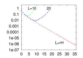
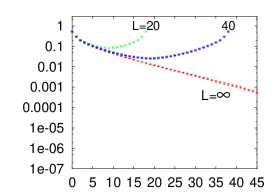
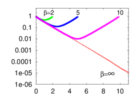
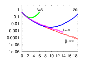
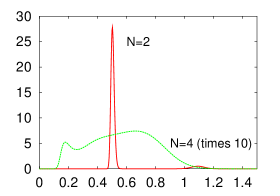
Figure 8: Left: Equal time staggered spatial correlation function of isotropically coupled Heisenberg antiferromagnetic chains, at $q_{\perp}=\pi$ and $\beta=\infty$, for N=2 (top) and N=4 chains (bottom).  Center: Greens functions $\langle S(\vec{q},0)\,S(\vec{q},t)\rangle$ at $\vec{q}=(\pi,\pi)$ for $L=\infty$, the infinite size system, with $N=2$ (top) and $N=4$ (bottom). Results at $L=20$, $\beta=\infty$ have been added to exemplify finite size effects. Right: Spectrum $S(\vec{q},\omega)$ at $\vec{q}=(\pi,\pi)$ for $L=\infty$ and $\beta=\infty$. From ref. [92].

As an example we show results for a spin ladder system [95] with $N=2$ and $4$ legs for the isotropic antiferromagnet ($\lambda=1$). The left side of figure 8 provides results for the equal time staggered spatial correlation functions along the chains. A fit to the infinite lattice result gives $\xi=2.93(2)$ for $N=2$ and $\xi=8.2(1)$ for $N=4$. The center part of figure 8 shows greens functions for $L=\infty$, the infinite size system. Whereas finite temperature calculations give results periodic in imaginary time, which have to be extrapolated, this approach provides the $\beta=\infty$ ($T=0$) result directly. A fit to the exponential decay $G(\tau)\sim e^{-\tau\Delta}$ directly provides estimates for the gaps $\Delta=0.5059(4)$ at $N=2$ and $\Delta=0.19(1)$ at $N=4$, consistent with previous calculations.Results for $L=20$ and $\beta=\infty$ are also shown, to exemplify the effect of finite size systems.

Continuing the imaginary time greens function to real frequencies by the maximum entropy method provides the spectra on the right side of figure 8, in which the gaps, the single magnon peaks, and higher excitations for $N=4$ are clearly visible.

2.16 Performance

The most important advantages and limitations of the loop algorithm have already been summarized in the introduction. Let us be more explicit here. Further aspects of the performance are mentioned in the following sections.

Autocorrelations: The biggest obstacle which the loop algorithm addresses are the long autocorrelation times of worldline algorithms with local updates, as discussed in the appendices (see eq. (B.11)). They require a proportional increase in computer time, so that simulations for large systems and/or low temperatures quickly become impossible. The loop algorithm appears to remove these autocorrelations completely in many cases (without magnetic field), like the spin $1\over 2$ Heisenberg AF in any dimension, the two-dimensional spin $1\over 2$ XY-model, and the spin $1$ Heisenberg chain. For large systems and low temperatures this can save many orders of magnitude in computer time. As one striking example, see the gain in autocorrelation time for the one-dimensional Hubbard model in figure 11 in section 4.7.

Autocorrelations and critical slowing down have been carefully determined in the original loop algorithm paper [1] for the nonquantum six-vertex model, with the single-cluster variant of the loop algorithm. In [96], a related study was done in which spatial winding was allowed to vary, with similar results for autocorrelations. In the massless phase (infinite correlation length) at $\frac{a}{c}=\frac{b}{c}=\sqrt{2}$, the loop algorithm completely eliminates critical slowing down, i.e. the autocorrelation times are small and constant. The dynamical critical exponent of the Monte Carlo method (see appendix B) was $z^{MC}_{int}\approx 0$ for all measured quantities, and $z^{MC}_{exp}=0.19(2)$ (or logarithmic dependence). On the KT transition line, the exponential autocorrelation times are slightly larger (up to $20$ on a $256^{2}$ lattice), with $z^{MC}_{exp}=0.71(5)$, yet for the integrated autocorrelation times, which are relevant for MC errors, we saw barely any autocorrelations in either case, up to the largest lattices of size $256^{2}$. Note that thus the dynamical critical exponent for the integrated autocorrelation time is zero here, different from that for the exponential autocorrelation time. Local updates, in contrast, indeed showed very long autocorrelation times, and $z^{MC}=2.2(2)$, as expected.

Other studies have also seen very small integrated autocorrelation times for quantum systems, not significantly increasing with $L$ or $\beta$, with both the single- and the multi-cluster version of the loop-algorithm for Heisenberg spin $1\over 2$ systems in 1d, 2d and on bilayers [97], a spin-$1$ ladder [98], and for a $t$-$J$ chain [42]. Note that away from a critical point, integrated autocorrelation times can even decrease with increasing system size, due to self-averaging of observables [97].

Strong fields (resp. chemical potentials) can however seriously impair the performance. They are discussed in section 4.3 and 4.4. See also section 5.3.

Improved Estimators: The use of improved estimators (section 2.14) provides additional gains. For example, in ref [99] it has been possible to calculate the spin-spin correlation function (which in standard updates has large variance) down to values of $10^{-5}$.

Change of global quantities: Since the loops are determined locally by the breakup decisions, they can easily, “by chance”, wind around the lattice in temporal or in spatial direction. An example is given in figure 6. The flip of such a loop then changes a global quantity (magnetization, particle number, spatial winding number). (Of course one can also choose to restrict the simulation to part of the total phase space, e.g. the canonical ensemble by not allowing such flips). This kind of configuration change is virtually impossible with standard local methods. It has been used to investigate e.g. the KT transition in the quantum XY model [100, 101].

Freezing: For the loop algorithm itself, apart from effects of global weights, models which require finite freezing weights $w^{ii}$ could potentially be difficult. The intuitive argument can easily be understood. If two different loops meet at a “frozen” plaquette (i.e. one for which the breakup $G^{ii}$ was chosen), they are glued together. If this happens at overly many plaquettes, then the cluster of glued loops which must be flipped together can occupy most of the lattice. The flip of such a cluster is not an effective move in phase space. It is basically equivalent to flipping all of the (few !) spins outside of that cluster. As an example, in ref. [1] we also investigated versions of the loop algorithm in which $w^{ii}$ was (unnecessarily !) chosen finite. Sizeable autocorrelations were the result. Minimal freezing, on the other hand, appears not to be a problem. (Ref. [102] includes freezing but also a large magnetic field). As an example, note that as mentioned in section 2.7 [55], the limiting case $J_{x,y}\!\rightarrow\!0$ of the loop algorithm is the classical Swendsen-Wang cluster algorithm, in which “freezing” is the only operation. Yet this cluster algorithm also drastically reduces critical slowing down in the corresponding classical models. More general cases with minimal freezing have apparently not been tested. For alternatives to freezing see also sections 3.3 and 5.3.

Implementation: Implementation of the loop algorithm in imaginary time is actually considerably easier than for local updates, which, especially in more than one dimension, require rather complicated local updates [88].

In section 2.13 it was explained how the time continuum limit $\Delta\tau\!\rightarrow\!\,0$ can be taken immediately in the loop algorithm, eliminating the Trotter approximation, reducing storage and CPU-time, and thus further extending the accessible temperature range. The implementation within the stochastic series expansion appears to be even more efficient, because of the discrete time-like variable used there. See section 3.6.

The loop algorithm can be vectorized and parallelized similarly to the Swendsen Wang cluster algorithm (see e.g. [84, 87]). A vectorized version was used in ref. [100, 101]. Vectorization or parallelization of the breakup process is trivial. The computationally dominant part is to identify the resulting clusters. This is equivalent to the well know problem of connected component labeling. See, e.g., ref. [103]. The optimal strategies are different from the Swendsen Wang case, because loops are linear objects. Efficient parallelization has been discussed by Todo [85, 86]. Each of $N_{p}$ nodes processes a slice of imaginary time of thickness $\beta/N_{p}$, identifying the loops that close withing a slice. The remaining unclosed loops are merged gradually by combining adjacent pairs of slices and iterating this process in a binary tree fashion, which produces only logarithmic overhead.

3 Operator formulation of the loop algorithm

A simple and straightforward derivation of the Loop Algorithm can be given directly on the operator level, instead of working on the level of matrix elements, as we have done so far. We will rewrite the Hamiltonian of our standard example, the Heisenberg $XXZ$ model, in terms of loop-operators, which are equivalent to the breakups introduced previously.

We can then directly write $tr\;e^{-\beta\hat{H}}$ as a continuous time path integral over loop-operators and spin variables (worldlines). Alternatively, we can express $tr\;e^{-\beta\hat{H}}$ with the stochastic series expansion (SSE) [6, 7, 8], arriving at a version of the complete loop algorithm within SSE.

Various parts of this formulation have appeared in the literature in different guises, especially in the operator formulation (on matrix element level) by Brower et al. [12], in the independent work by Aizenman and Nachtergaele on the Heisenberg model [10, 11], in Sandvik’s work on the interaction representation [104] and on “operator loop updates” for the isotropic AF [13], in the work by Harada and Kawashima [14], and in connection with the meron approach [27, 28, 29, 31].

3.1 Isotropic Antiferromagnet

The Hamiltonian of the spin $1\over 2$ Heisenberg XXZ model on a single lattice bond ${\left<ij\right>}$, without field, is given by eq. (2.1)

$$\hat{H}_{ij}~{}=~{}J_{x}(\hat{S}^{x}_{{i}}\hat{S}^{x}_{{j}}+\hat{S}^{y}_{{i}}\hat{S}^{y}_{{j}})+J_{z}\hat{S}^{z}_{{i}}\hat{S}^{z}_{{j}}\;.$$ (3.1)

For the isotropic antiferromagnet $J_{x}=J_{z}=J>0$, we rewrite

$$\begin{array}[]{lllllllll}-\frac{1}{J}\,\hat{H}_{ij}\;+\;\frac{1}{4}\par&=&-\,\vec{\hat{S}}_{i}\vec{\hat{S}}_{j}\;+\;\frac{1}{4}\\[6.45831pt] &=&-{1\over 2}(\hat{S}^{+}_{{i}}\hat{S}^{-}_{{j}}+\hat{S}^{-}_{{i}}\hat{S}^{+}_{{j}})\;-\;\left(\hat{S}^{z}_{{i}}\hat{S}^{z}_{{j}}\;-\;\frac{1}{4}\right)\\[6.45831pt] &=&\frac{1}{2}\left(~{}-\begin{minipage}{30.1388pt}\hskip 0.30121pt \includegraphics[width=18.08345pt]{Figures/crossleft.eps} \end{minipage}-\begin{minipage}{30.1388pt}\hskip 0.30121pt \includegraphics[width=18.08345pt]{Figures/crossright.eps} \end{minipage}+\begin{minipage}{30.1388pt}\hskip 0.30121pt \includegraphics[width=18.08345pt]{Figures/leftup.eps} \end{minipage}+\begin{minipage}{30.1388pt}\hskip 0.30121pt \includegraphics[width=18.08345pt]{Figures/rightup.eps} \end{minipage}~{}\right)\\[12.91663pt] &=&\frac{1}{\sqrt{2}}\left(\,\left|\uparrow\downarrow\right\rangle-\left|\downarrow\uparrow\right\rangle\,\right)~{}\frac{1}{\sqrt{2}}\left(\,\left\langle\uparrow\downarrow\right|-\left\langle\downarrow\uparrow\right|\,\right)\;.\end{array}$$ (3.2)

This operator acts towards the right, except for the third line, where we have given a worldline-like picture for illustration, to be interpreted as an operator acting towards the bottom. We have added a constant $\frac{1}{4}$ to eliminate the contributions of parallel spins. We see that the bond operator $\hat{H}_{ij}$ of the Heisenberg antiferromagnet is $-J$ times a singlet projection operator.

On a bipartite lattice we can change the sign of $J_{x}$ (see footnote 4), obtaining the operator $\tilde{\hat{H}}_{ij}$, equivalent to $\hat{H}_{ij}$, with

$$\begin{array}[]{lllllllll}-\frac{1}{J}\,\tilde{\hat{H}}_{ij}\;+\;\frac{1}{4}\par\par&=&\frac{1}{\sqrt{2}}\left(\,\left|\uparrow\downarrow\right\rangle+\left|\downarrow\uparrow\right\rangle\,\right)~{}\frac{1}{\sqrt{2}}\left(\,\left\langle\uparrow\downarrow\right|+\left\langle\downarrow\uparrow\right|\,\right)\\[6.45831pt] &=&\frac{1}{2}\left(~{}\begin{minipage}{30.1388pt}\hskip 0.30121pt \includegraphics[width=18.08345pt]{Figures/crossleft.eps} \end{minipage}+\begin{minipage}{30.1388pt}\hskip 0.30121pt \includegraphics[width=18.08345pt]{Figures/crossright.eps} \end{minipage}+\begin{minipage}{30.1388pt}\hskip 0.30121pt \includegraphics[width=18.08345pt]{Figures/leftup.eps} \end{minipage}+\begin{minipage}{30.1388pt}\hskip 0.30121pt \includegraphics[width=18.08345pt]{Figures/rightup.eps} \end{minipage}~{}\right)\\[12.91663pt] &=&\frac{1}{2}\left(~{}\begin{minipage}{30.1388pt}\hskip 0.30121pt \includegraphics[width=18.08345pt]{Figures/breakhll.eps} \end{minipage}~{}+~{}\begin{minipage}{30.1388pt}\hskip 0.30121pt \includegraphics[width=18.08345pt]{Figures/breakrr.eps} \end{minipage}~{}+~{}\begin{minipage}{30.1388pt}\hskip 0.30121pt \includegraphics[width=18.08345pt]{Figures/breaklr.eps} \end{minipage}~{}+~{}\begin{minipage}{30.1388pt}\hskip 0.30121pt \includegraphics[width=18.08345pt]{Figures/breakrl.eps} \end{minipage}~{}\right)\\[12.91663pt] &=:&\frac{1}{2}\begin{minipage}{30.1388pt}\hskip 0.30121pt \includegraphics[width=18.08345pt]{Figures/breakh.eps} \end{minipage}~{}~{}\equiv~{}~{}\frac{1}{2}\;\hat{B}^{h}_{ij}~{}.\end{array}$$ (3.3)

On the third line we have again written a worldline-like picture. The arrows (spin directions) remain the same on the fourth line, but we have now chosen to connect them differently, while keeping continuity of arrows along the connecting lines. As a result we see that the contributions to $\tilde{\hat{H}}_{ij}$ with nonzero matrix elements are the same as those contributing to a horizontal loop-breakup. Thus the horizontal breakup can be written as an operator

$$\hat{B}^{h}_{ij}~{}\equiv~{}\begin{minipage}{30.1388pt}\hskip 0.30121pt \includegraphics[width=18.08345pt]{Figures/breakh.eps} \end{minipage}~{}=~{}\left(\,\left|\uparrow\downarrow\right\rangle+\left|\downarrow\uparrow\right\rangle\,\right)~{}\left(\,\left\langle\uparrow\downarrow\right|+\left\langle\downarrow\uparrow\right|\,\right)~{},$$ (3.4)

with $\frac{1}{2}\hat{B}^{h}_{ij}$ a projection operator. After sublattice rotation on a bipartite lattice, the energy-shifted Heisenberg bond-operator is therefore the same as a horizontal breakup, on an operator level.

In passing, we also note that the vertical breakup of the loop-algorithm is just the identity operator

$$\begin{minipage}{30.1388pt}\hskip 0.30121pt \includegraphics[width=18.08345pt]{Figures/breakv.eps} \end{minipage}~{}\equiv~{}\hat{B}^{v}_{ij}~{}\equiv~{}1\!\!1~{}.$$ (3.5)

The partition function eq. (2.3) of the antiferromagnet ($J>0$) on a bipartite lattice becomes

$$Z=tr\,e^{-\beta\hat{H}}~{}=~{}\;e^{\beta\frac{J}{2}\sum_{{\left<ij\right>}}(\hat{B}^{h}_{ij}-\frac{1}{2})}~{}.$$ (3.6)

3.2 Isotropic Ferromagnet

The ferromagnet can be treated in the same way. Now $J_{x}=J_{z}=J<0$, and

$$\begin{array}[]{lllllllll}-\frac{1}{|J|}\,\hat{H}_{ij}~{}+~{}\frac{1}{4}\par&=&\vec{\hat{S}}_{i}\vec{\hat{S}}_{j}\;+\;\frac{1}{4}\\[6.45831pt] &=&{1\over 2}(\hat{S}^{+}_{{i}}\hat{S}^{-}_{{j}}+\hat{S}^{-}_{{i}}\hat{S}^{+}_{{j}})\;+\;\left(\hat{S}^{z}_{{i}}\hat{S}^{z}_{{j}}\;+\;\frac{1}{4}\right)\\[6.45831pt] &=&\frac{1}{2}\left(~{}\begin{minipage}{30.1388pt}\hskip 0.30121pt \includegraphics[width=18.08345pt]{Figures/crossleft.eps} \end{minipage}+\begin{minipage}{30.1388pt}\hskip 0.30121pt \includegraphics[width=18.08345pt]{Figures/crossright.eps} \end{minipage}+\begin{minipage}{30.1388pt}\hskip 0.30121pt \includegraphics[width=18.08345pt]{Figures/upup.eps} \end{minipage}+\begin{minipage}{30.1388pt}\hskip 0.30121pt \includegraphics[width=18.08345pt]{Figures/downdown.eps} \end{minipage}~{}\right)\\[12.91663pt] &=&\frac{1}{2}\left(~{}\begin{minipage}{30.1388pt}\hskip 0.30121pt \includegraphics[width=18.08345pt]{Figures/crossleft.eps} \end{minipage}+\begin{minipage}{30.1388pt}\hskip 0.30121pt \includegraphics[width=18.08345pt]{Figures/crossright.eps} \end{minipage}+\begin{minipage}{30.1388pt}\hskip 0.30121pt \includegraphics[width=18.08345pt]{Figures/crossupup.eps} \end{minipage}+\begin{minipage}{30.1388pt}\hskip 0.30121pt \includegraphics[width=18.08345pt]{Figures/crossdowndown.eps} \end{minipage}~{}\right)\\[12.91663pt] &=&\frac{1}{2}\begin{minipage}{30.1388pt}\hskip 0.30121pt \includegraphics[width=18.08345pt]{Figures/breakd.eps} \end{minipage}~{}~{}\equiv~{}~{}\frac{1}{2}\;\hat{B}^{d}_{ij}~{}.\par\end{array}$$ (3.7)

Here the constant $\frac{1}{4}$ was chosen to eliminate the contributions of antiparallel spins. On the third line we have again written a worldline-like picture. The arrows (spin directions) remain the same on the fourth line, but we have again chosen to connect them differently, while keeping continuity of arrows along the connecting lines. As a result we see that for the isotropic ferromagnet on any lattice, the operator $\tilde{\hat{H}}_{ij}$, after an energy-shift, is proportional to the operator $\hat{B}^{d}_{ij}$ for a diagonal loop-breakup, which indeed is the permutation operator.

The partition function eq. (2.3) of the ferromagnet on any lattice becomes

$$Z=tre^{-\beta\hat{H}}~{}=~{}\;e^{\beta\frac{|J|}{2}\sum_{{\left<ij\right>}}(\hat{B}^{d}_{ij}-\frac{1}{2})}~{}.$$ (3.8)

Note that the difference between antiferromagnet and ferromagnet is connected to requiring positivity of the final exponent for the partition function, leading to horizontal breakups for the antiferromagnet and diagonal ones for the ferromagnet.

3.3 Anisotropy

To treat models with anisotropy $\Delta=J_{z}/|J_{x}|$, we can use the operator identities

$$\begin{array}[]{lllllllll}4\;S_{i}^{z}S_{j}^{z}\par&=&\begin{minipage}{30.1388pt}\hskip 0.30121pt \includegraphics[width=18.08345pt]{Figures/breakd.eps} \end{minipage}~{}-~{}\begin{minipage}{30.1388pt}\hskip 0.30121pt \includegraphics[width=18.08345pt]{Figures/breakh.eps} \end{minipage}~{},\end{array}$$ (3.9)

which follows by subtracting eq. (3.3) from eq. (3.7), and

$$\begin{array}[]{lllllllll}2\left(\hat{S}^{+}_{{i}}\hat{S}^{-}_{{j}}+\hat{S}^{-}_{{i}}\hat{S}^{+}_{{j}}\right)&=&\begin{minipage}{30.1388pt}\hskip 0.30121pt \includegraphics[width=18.08345pt]{Figures/breakd.eps} \end{minipage}~{}+~{}\begin{minipage}{30.1388pt}\hskip 0.30121pt \includegraphics[width=18.08345pt]{Figures/breakh.eps} \end{minipage}~{}-~{}1\!\!1~{}.\end{array}$$ (3.10)

For the antiferromagnet on a bipartite lattice we get

$$\begin{array}[]{lllllllll}-\frac{1}{|J_{x}|}\tilde{\hat{H}}_{ij}&=&\frac{1+\Delta}{4}\begin{minipage}{30.1388pt}\hskip 0.30121pt \includegraphics[width=18.08345pt]{Figures/breakh.eps} \end{minipage}~{}+~{}\frac{1-\Delta}{4}\begin{minipage}{30.1388pt}\hskip 0.30121pt \includegraphics[width=18.08345pt]{Figures/breakd.eps} \end{minipage}~{}-~{}\frac{1}{4}~{}.\end{array}$$ (3.11)

The anisotropic ferromagnet on any lattice is given by the same equation, with $\Delta<0$. These results are equivalent to eq. (2.39). They provide positive weights when $|\Delta|\leq 1$.

Freezing and alternatives

For $\Delta>1$, i.e. the Ising-like regions of parameter space, the operator formulation leads to, e.g., the following approaches:

• One possibility is to use $(S_{i}^{z}S_{j}^{z}\pm\frac{1}{4})$ as an operator, with weight $\Delta-1$. Then on bonds where this operator acts, the weight of a configuration with AF (or FM) neighboring spins is zero, i.e. forbidden. This amounts to an operator formulation of freezing of the opposite spin orientation (see section 2.5).

• Alternatively, one can use $S_{i}^{z}S_{j}^{z}$ as an operator, and proceed similarly to the case of merons (section 4.8). The flip of a loop connected to some other loop by an odd number of such operators will result in a sign flip for the total weight of the configuration, and therefore in a combined contribution of zero to the total weight. Thus only configurations with an even number of such connections contribute, while keeping loops independent.

• An interesting different alternative has been developed by Otsuka [105]: He treats $(\Delta-1)S_{i}^{z}S_{j}^{z}$ by introducing Hubbard-Stratonovich variables, which act locally like a magnetic field. Then loop flips remain independent, with a flip probability that depends on the Hubbard-Stratonovich configuration.

3.4 Treating $e^{-\beta\hat{H}}$ as a continuous imaginary time path integral

We can obtain the path integral in continuous imaginary time by directly employing a Poisson process representation of $e^{-\beta\hat{H}}$, as specified rigorously by Aizenman and Nachtergaele (section 2.2 of reference [10]). For related work see [90, 89]. Rephrased for our context the statement refers to a Hamiltonian of the form

$$\hat{H}=-\sum_{b}J_{b}\,\hat{h}_{b}$$ (3.12)

with bonds $b$, nonnegative couplings $J_{b}$, and selfadjoint operators $\hat{h}_{b}$, which acts on a finite system. Then $e^{-\beta\hat{H}}$ can be expressed as a Poisson integral:

$$\begin{array}[]{lllllllll}e^{-\beta\hat{H}}&=e^{\beta\sum_{b}J_{b}}\lim_{\Delta t\to 0}\left({\prod}_{b}e^{(-J_{b}+J_{b}\hat{h}_{b})\Delta t}\right)^{\beta/\Delta t}\\[6.45831pt] &=e^{\beta\sum_{b}J_{b}}\lim_{\Delta t\to 0}\left({\prod}_{b}\{(1-J_{b}\Delta t)+J_{b}\hat{h}_{b}\Delta t\}\right)^{\beta/\Delta t}\\[6.45831pt] &=e^{\beta\sum_{b}J_{b}}\int\rho(d\omega)\prod^{*}\hat{h}_{b}~{},\end{array}$$ (3.13)

where $\prod^{*}\hat{h}_{b}$ is a time ordered product of bond operators $\hat{h}_{b}$, $\omega$ is the bond configuration, and $\rho(d\omega)$ is a poissonian probability measure with density $\prod_{b}J_{b}dt$. Thus, we get a random countable collection of time-indexed bonds which occur independently in disjoint regions of spacetime. This is a non-commutative version of the usual power series expansion of the exponential function.

Loop operator representation

If we choose to represent the antiferromagnet as a sum over horizontal loop operators,

$$\hat{H}~{}+~{}const~{}~{}=~{}~{}-\frac{J}{2}\;\sum_{\left<ij\right>}\;\hat{B}^{h}_{ij}~{},$$ (3.14)

then the theorem states that we can represent $e^{-\beta\hat{H}}$ as stochastic integral over configurations of loop operators $\hat{B}^{h}_{ij}$ which appear with constant probability density $J/2$ in continuous imaginary time. In between these operators there is just the identity operator, to which we have been referring as a vertical breakup. Quantizing in $S^{z}$ basis, one obtains continuous lines between the loop operators. Finally, taking the trace of $e^{-\beta\hat{H}}$ provides periodic boundary conditions in imaginary time for the resulting configuration of horizontal loop operators and lines.

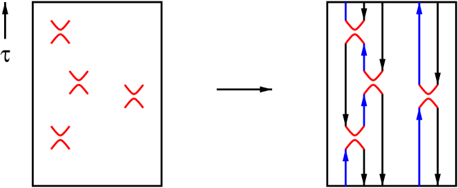
Figure 9: Configuration of horizontal loop operators (left), and a compatible loop and (world)line configuration (right).

Since these lines do not start anywhere, they close to form loops, with two possible orientations of arrows (spins) on each loop. When the spin points upwards, these lines are worldlines. From eq. (3.3) we see that all matrix elements are unity, so the total weight of the configuration (once stochastically chosen) is unity.

We have arrived at the combined loop-operator and spin representation of the Heisenberg model in continuous time. From this representation we can immediately derive the loop algorithm as a Quantum Monte Carlo procedure by switching back and forth between (i) choosing a new operator configuration compatible with the current spin configuration, with probability density $J/2$ for each operator, and (ii) choosing a new spin configuration compatible with the current operator configuration. This is the same procedure as that derived in section 2.13.

When we sum over all possible spin configurations, two for each loop, we obtain the pure-loop representation of the Heisenberg model (see section 2.10).

Standard hopping representation

We can also stay in the standard representation eq. (3.1), in which the operators $S^{+}S^{-}$ correspond to hopping of worldlines, and $4S^{z}_{i}S^{z}_{j}\pm 1$ is diagonal, both with matrix elements unity or zero.

Then we obtain a standard worldline representation, but directly in continuous time. Thus the existence of a continuous time representation is independent of whether one uses a loop representation [89]. Here one can perform, e.g., something like the usual local updates of standard worldline Monte Carlo, e.g. by proposing to shift an existing hopping operator $S^{+}S^{-}$ by some time $\Delta\tau$, uniformly chosen within a suitable range.

3.5 Treating $e^{-\beta\hat{H}}$ by stochastic series expansion

The stochastic series expansion of an operator $e^{-\beta\hat{H}}$, was introduced by Anders Sandvik [6, 7, 8]. It is related to the Handscomb method [77, 78, 79, 80, 81] for the Heisenberg model, but also applicable to many other models. We assume again that $\hat{H}=\sum_{\nu,b}\hat{H}_{\nu,b}$ is a sum of operators $\hat{H}_{\nu,b}$ living on bonds $b$. (Site terms can also be brought into this form). SSE proceeds from the power series

$$\begin{array}[]{lllllllll}e^{-\beta\hat{H}}&=&\sum_{n=1}^{\infty}\;\frac{\beta^{n}}{n!}\;(-\hat{H})^{n}\\[6.45831pt] &=&\sum_{n=1}^{\infty}\;\frac{\beta^{n}}{n!}\;(-\hat{H}_{1}-\hat{H}_{2}-...)(-\hat{H}_{1}-\hat{H}_{2}-...)...\\[6.45831pt] &=&\sum_{n=1}^{\infty}\;\frac{\beta^{n}}{n!}\;\sum_{j_{1},j_{2},...,j_{n}}(-\hat{H}_{j_{1}})(-\hat{H}_{j_{2}})...(-\hat{H}_{j_{n}})~{},\par\end{array}$$ (3.15)

where $j$ is a shorthand for $(\nu,b)$. The third line is obtained by expanding the product in the second line, resulting in a sum with one sub-Hamiltonian $\hat{H}_{j_{k}}$ from each of the $n$ factors. For a fixed value of $n$, we obtain a sum over sequences of $n$ operators $\hat{H}_{j_{k}}$. There is now a discrete index $l=1..n$ with “time-like” properties, since it describes a sequence of Hamiltonians. At each value of $l$, only one of the sub-Hamiltonians acts. The partition function becomes

$$Z~{}=~{}\sum_{\alpha}\,\sum_{n=0}^{\infty}\,\sum_{S_{n}}\,\frac{\beta^{n}}{n!}\;\left\langle\alpha\right|\,\prod\,(-\hat{H}_{(\nu,b)_{i}})\,\left|\alpha\right\rangle$$ (3.16)

where $S_{n}$ is a sequence $((\nu,b)_{1},(\nu,b)_{2},...,(\nu,b)_{n})$ of operator indices. We insert $\hat{S}^{z}$ eigenstates for $\left|\alpha_{l}\right\rangle$ between all operators. The result is again a worldline-like representation of $tr\;e^{-\beta\hat{H}}$, this time with a discrete index space instead of continuous imaginary time.

Let us emphasize that the stochastic series expansion, as presented so far, is a different treatment of $e^{-\beta\hat{H}}$, independent of the choice of sub-Hamiltonians and of any Monte Carlo procedure. We also note that the continuous time representation eq. (3.13), with a time ordered set of sub-Hamiltonians, and the stochastic series expansion are indeed closely related. The biggest difference is the discreteness of index space in case of SSE. This discreteness increases the efficiency of SSE with respect to continuous time.

Standard hopping representation

If we choose the standard hopping representation eq. (3.1), then local updates of the operator configuration, as specified in the original SSE papers, are the natural choice.

Loop operator representation

If instead we choose a loop operator representation like eq. (3.14), then we arrive again at a combined worldline/loop-operator representation of $tr\;e^{-\beta\hat{H}}$. Switching back and forth between choosing operators and choosing worldlines results in the loop algorithm, this time in discrete index space. For the isotropic Heisenberg antiferromagnet and ferromagnet, a variant of this procedure was introduced by Sandvik as “operator loops with deterministic updates” [13, 32], developed from a different approach (section 5.2). From the present formulation we see that indeed the complete loop algorithm can be applied within SSE, including anisotropic cases and generalizations.

3.6 Loop algorithm in SSE

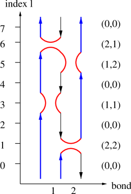
Figure 10: Part of an SSE configuration in loop-operator representation. The diagonal operator $1\!\!1$ is drawn as a vertical breakup. A compatible spin-configuration is denoted by the arrows. The vertical axis marks the propagation index $l$, the horizontal axis numbers bonds $b$. The sequence $(\nu,b)$ is given on the right, with $\nu=1$ ($\nu=2$) denoting a vertical (horizontal) breakup.

Let us describe a possible implementation of the loop algorithm with SSE in more detail. The continuous time version was described in section 2.13. For further information, we refer to the literature on SSE [6, 7, 8, 13, 97, 48].

We describe the case of an anisotropic Heisenberg model on a bipartite lattice. From eq. (3.11) we get (with $J_{x}=1$ as unit of energy)

$$\begin{array}[]{lllllllll}-\hat{H}_{ij}\par&:=&-\frac{1}{2}(\hat{S}^{+}_{{i}}\hat{S}^{-}_{{j}}+\hat{S}^{-}_{{i}}\hat{S}^{+}_{{j}})\;-\;\Delta\;\hat{S}^{z}_{{i}}\hat{S}^{z}_{{j}}\;+\;\frac{1}{4}\;+\;\epsilon\,1\!\!1\\[6.45831pt] &=&\frac{1+\Delta}{4}\begin{minipage}{30.1388pt}\hskip 0.30121pt \includegraphics[width=18.08345pt]{Figures/breakh.eps} \end{minipage}~{}+~{}\frac{1-\Delta}{4}\begin{minipage}{30.1388pt}\hskip 0.30121pt \includegraphics[width=18.08345pt]{Figures/breakd.eps} \end{minipage}~{}+~{}\epsilon\,1\!\!1\\[6.45831pt] &=:&J_{h}\hat{B}^{h}~{}+~{}J_{d}\hat{B}^{d}~{}+~{}\epsilon\,\hat{D}\end{array}$$ (3.17)

with $|\Delta|\leq 1$, $\epsilon>0$ and a “diagonal operator” $\hat{D}=1\!\!1$. We have added a constant to $\hat{H}_{ij}$ to ensure positivity of matrix elements. The constant $\epsilon$ might be varied to further improve convergence [48].

It is advantageous to extend the SSE sequence to a fixed length $L$ by introducing additional “empty” unit operators $\hat{h}^{0}=1\!\!1$. Then [8]

$$Z~{}=~{}\sum_{\alpha}\,\sum_{S_{L}}\,\frac{\beta^{n}(L-n)!}{L!}\left\langle\alpha\right|\,\prod_{i=1}^{L}(-\hat{H}_{(\nu,b)_{i}})\,\left|\alpha\right\rangle$$ (3.18)

with $n$ the number of non-unit operators in the sequence $S_{L}$. This can be done without approximation in practice, since the average length of the operator string is just the total energy of the system, as seen by differentiating with respect to $\beta$, and its fluctuations are finite in any finite run. A value for $L$ with a safe margin can be determined during thermalization.

The SSE configuration is specified by $S_{n}$, which can be written as a sequence of tuples $(\nu,b)$, with $(0,0)$ denoting $\hat{h}^{0}$. When the operators $\hat{H}_{(}\nu,b)$ are “non-branching”, it suffices to specify the initial state $\alpha(0)$. Otherwise (as for horizontal loop-operators), the “worldline configuration” $\left|\alpha(l)\right\rangle$ has to be stored, too. A picture of an SSE configuration is shown in figure 10.

The simulation begins with, e.g., a configuration of all down spins and $S_{n}$ consisting of only empty operators.

An overall Monte-Carlo-update consists of three parts. First, empty operators $\hat{h}^{0}$ and diagonal operators operators $\hat{D}$ are exchanged with Metropolis probability.

$$\begin{array}[]{lllllllll}p(\,(0,0)_{l}\rightarrow(1,b)_{l}\,)~{}=~{}\min\left(1,\frac{N_{b}\,\beta\,\left\langle\alpha(l)\right|\hat{D}_{b}\left|\alpha(l)\right\rangle}{L-n}\right)\\[6.45831pt] p(\,(1,b)_{l}\rightarrow(0,0)_{l}\,)~{}=~{}\min\left(1,\frac{L-n+1}{N_{b}\,\beta\,\left\langle\alpha(l)\right|\hat{D}_{b}\left|\alpha(l)\right\rangle}\right)\end{array}$$ (3.19)

where $N_{b}$ is the total number of bonds and $\nu=1$ stands for the diagonal operator $\hat{D}$. This step changes the expansion order $n$ by $\pm 1$. It is attempted consecutively for each $l=1,...,L$.

In the second step, the “breakup decision”, diagonal operators $\hat{D}$ and loop-operators $\hat{B}^{h}$, $\hat{B}^{d}$ are exchanged. Now only the “vertices” with non-empty operators matter. As in the case of continuous time, one needs a doubly linked list connecting each of the four “legs” of each vertex with the corresponding leg of the next (resp. previous) vertex. The information on spins can be stored with the vertices.

As usual at each vertex, the local spin configuration allows two of the three breakups, vertical (operator $\hat{D}$), horizontal $\hat{B}^{h}$ or diagonal $\hat{B}^{d}$. The choice is made at each vertex with heat-bath probability. Thus on an antiferromagnetic vertex (like plaquettes $2^{\pm}$ in fig. 3), the horizontal breakup in our example is chosen with probability

$$\frac{1+\Delta}{4\epsilon\,+\,(1+\Delta)}$$ (3.20)

and on a vertex with spin-flip (like plaquettes $3^{\pm}$) it is chosen with probability

$$\frac{\frac{1}{4}(1+\Delta)}{\frac{1}{4}(1-\Delta)\,+\,\frac{1}{4}(1+\Delta)}~{}=~{}\frac{1}{2}(1+\Delta)~{}.$$ (3.21)

The third step consists as ususal of identifying and flipping loops. Nontrivial diagonal operators as well as external fields can influence the flip probability. Note that on sites on which no operators act there is a straight loop.

The “deterministic operator-loops” previously constructed [13] for isotropic ferro- and antiferromagnet are somewhat different. They use a different diagonal operator in eq. (3.17) which forbids ferromagnetic vertex configurations. The generalization of the loop algorithm just outlined has lower autocorrelations, as recently shown by Syljuasen and Sandvik [48].

We have described the multi-cluster loop-algorithm. In the single cluster version, loop construction starts at a randomly chosen vertex-leg, and decides breakups iteratively until the loop closes. (This construction generalizes to the directed loops in section 5.3, which are better suited, e.g., for large magnetic fields.)

Measurements of static observables are straightforward [104]. For example, the total energy is given by $E=\-\frac{1}{\beta}\,\langle n\rangle$ and the heat capacity by

$$C_{V}~{}=~{}\langle n^{2}\rangle\;-\;\langle n\rangle^{2}\;-\;\langle n\rangle~{}.$$ (3.22)

Time-dependent correlations are also available [8]. An imaginary time separation $\tau$ corresponds to a binomial distribution of propagation distances $\Delta l$, and correlators are given by

$$\langle\hat{A}(\tau)\,\hat{B}(0)\rangle~{}=~{}\left\langle\sum_{\Delta l=0}^{n}\,\left(n\atop{\Delta l}\right)\,\left(\frac{\tau}{\beta}\right)^{\Delta l}\,\left(1-\frac{\tau}{\beta}\right)^{n-\Delta l}C_{\hat{A}\hat{B}}(\Delta l)\,\right\rangle$$ (3.23)

with

$$C_{\hat{A}\hat{B}}(\Delta l)~{}=~{}\frac{1}{n+1}\,\sum_{l=0}^{n}\,\hat{B}(l+\Delta l)\,\hat{A}(l)~{}.$$ (3.24)

Improved observables are available as usual. An efficient method to measure time-dependent Greens functions has been provided by Dorneich and Troyer [97].

3.7 Discussion

We have seen that the issue of representing $tr\;e^{-\beta\hat{H}}$ by a (continuous or discrete) imaginary time path integral, or by SSE, is independent of the choice of representation of $\hat{H}$, e.g. in terms of traditional hopping operators, or in terms of loop operators, and independent of the resulting possible update procedures. The loop operator representation of $\hat{H}$ and the full loop algorithm can be applied both in the imaginary time path integral and in SSE. Additional operators in $\hat{H}$ can be treated similarly (see sections 3.3,4.4). Because of its discrete index space, the stochastic series expansion appears to be somewhat more efficient computationally than continuous imaginary time.

4 Generalizations

So far we have purposely restricted ourselves to XYZ-like models in order to simplify the presentation. This covered both the case of spin $1\over 2$ quantum spin models, where we have inserted eigenstates $\left|S^{z}_{il}\right>=\left|\pm 1\right>$ (or eigenstates along a different quantization axis) and models of fermions or hard core bosons, where we have inserted occupation number eigenstates [5]. We have developed the formalism for the general anisotropic XYZ-like (eight-vertex-like) case. We have computed explicit update probabilities for all XXZ and most XYZ-like cases.

Let us now describe further generalizations, several of which are immediate. For all generalizations, with a slight modification for continuous time (section 2.13), it remains true that locally on the vertices we have a situation like in the six- (or eight-) vertex model, so that the loop formulation, on the level of matrix elements or on the level of operators, described above can be applied directly.

4.1 Long range couplings

Hopping or spin-spin interactions beyond nearest neighbor can be handled by the same approach as higher dimensions, namely by introducing extra parts $\hat{H}_{\nu}$ in the split of the Hamiltonian, i.e. extra “bonds” on the lattice, with a corresponding set of shaded plaquettes living on separate Trotter time subslices.

When the number of additional couplings is large, this approach becomes impractical. It is somewhat less cumbersome in the continuous time version of the loop algorithm (section 2.13). A stochastic approach by Luijten and Blöte to extend cluster simulations to such cases may be helpful here [106].

4.2 Bond disorder, diluted lattices, and frustration

Bond disorder refers to spatial variations in the spin couplings $J_{ij}$ (resp. hopping strengths $t_{ij}$ and/or density-density couplings $V_{ij}$). This modifies the loop-construction probabilities locally, making them plaquette-dependent. Otherwise nothing changes ! (One does need to check whether ergodicity is still achieved.)

The same is true for diluted lattices, which can be viewed as a case of bond disorder in which the coupling vanishes completely on some bonds.

The situation is different for frustrated couplings whence some matrix elements become negative and cannot be transformed to a positive representation. Whereas the loop algorithm itself is unaffected, this produces a second type of sign problem which needs to be handled in the same way as the fermion sign problem (section 4.7). If the strength and/or frequency of frustrated matrix elements, as well as system size and $\beta$ are not too large, this sign problem can remain manageable [42, 107]. In general, however, it has so far precluded simulations of strongly frustrated models. It is possible to find improved estimators for frustrated couplings [42], to alleviate this sign problem. Note that for non-bipartite lattices, the breakup probabilities have to be modified to ensure ergodicity of the algorithm, as has been discussed in section 2.9. This modification might introduce additional freezing, which, however, is dwarfed by the sign problem.

Promisingly, the meron-strategy outlined in section 4.8 can also be applicable to frustrated systems. Indeed, this way Henelius and Sandvik have succeeded in simulating a “semi-frustrated” Heisenberg quantum spin system without sign problem [32], though at present other frustrated model. In special cases, one can also find a new basis without sign problem, e.g. for a Trellis lattice with special range of couplings [108, 109].

4.3 Asymmetric Hamiltonians: Magnetic field, chemical potential

Asymmetric weights can be caused by a (uniform or random) magnetic field in $\hat{S}^{z}$-direction or equivalently a chemical potential, or by other non “particle-hole-symmetric” terms, like e.g. softcore bosons. Large diagonal fields seriously affect the performance of the loop algorithm. Transverse fields, however, are easily handled (see section 4.4).

Within the algorithm presented so far, asymmetric parts of the Hamiltonian need to be taken into the global weight $A_{global}$, such that $W^{plaq}$ is symmetric with respect to a flip of all four spins on each shaded plaquette. Then they contribute to the flip probabilities $p_{flip}$ of the clusters.

A magnetic field $h$ (or chemical potential $\mu$) affects only clusters which change the number of worldlines, i.e. which wind around the lattice in temporal direction. The acceptance rate for the flip of such clusters is proportional to $\exp(-\beta hn_{w})$, where $n_{w}$ is the temporal winding number of the cluster. At sufficiently large values of $\beta h$ the acceptance rate becomes very small on average and results in an exponential slowing down of the simulation. This was indeed observed [110, 111, 97]. For such large diagonal fields, the “worm-algorithm”, and especially the general method of “directed loops”, discussed in section 5, are much better suited. When comparing computational effort for equal error bars for one- and two-dimensional Heisenberg systems, the threshold in comparison to SSE worms (see section 5.2) was $\beta h\raisebox{-3.0pt}{$\stackrel{{\scriptstyle>}}{{\sim}}$}3$ [97]. When comparing to the worm-algorithm for a Heisenberg-chain, the threshold was at $\beta h\raisebox{-3.0pt}{$\stackrel{{\scriptstyle>}}{{\sim}}$}5$ [111].

On the other hand, at small fields $\beta h\raisebox{-3.0pt}{$\stackrel{{\scriptstyle<}}{{\sim}}$}1$ it appears to be advantageous to use the loop algorithm with global acceptance step [97] to achieve equal errors with smaller computational effort.

To minimize the acceptance problem, one should normally choose $A_{global}$ such that its fluctuations are minimized. Somewhat surprisingly, it has also been reported [112] that supplementing the cluster updates with explicit global flips of worldlines helps considerably, even at rather larger values of $\beta h$. An interesting variant of the loop algorithm which appears to work well for very large diagonal fields was introduced by Syljuasen [113].

Let us note that the canonical ensemble (or ensemble of constant magnetization) is simulated by disallowing the flip of clusters which would change the number of worldlines. It is also possible, and can reduce autocorrelations, to allow the number of worldlines to fluctuate, and afterwards treat each subset of configurations with a certain number of worldlines as a canonical simulation [64, 65].

4.4 Transverse field

There is a different way to treat magnetic fields and chemical potentials, which can be simulated without difficulties. One can change the axis of quantization to turn a magnetic field into the x-direction. The field operator $\hat{S}^{x}=\frac{1}{2}\;(\!\begin{array}[]{cc}{\scriptstyle 0\,1}\\[-4.30554pt] {\scriptstyle 1\,0}\end{array}\!)$ then flips the direction of a spin. It can act at any spacetime point $(il)$. Worldlines now become piecewise continuous, with spin flips whereever $\hat{S}^{x}$ acts. For the isotropic Heisenberg model, the physics is invariant under this rotation.

Rieger and Kawashima [17] have shown how to treat such source operators in a cluster algorithm. They investigated the Ising model in a transverse field, for which $J_{x}=0$ and all worldlines are thus straight. Here we apply their method to the loop algorithm.

We enlarge our graph to consist not only of breakups but also of the information, for each spacetime site, whether $\hat{S}^{x}$ acts there or not. $\hat{S}^{x}$ occurs in matrix elements like $W_{h}\equiv\langle+|\exp{(\Delta\tau h\hat{S}^{x})}|-\rangle=\sinh{(\frac{\Delta\tau}{2}h)}$. Its presence or absence in a graph can be treated with Metropolis probability: Tentatively put additional operators $\hat{S}^{x}$ with probability $p=W_{h}$ on any lattice site where there is no $\hat{S}^{x}$ yet. After choosing breakups as usual we now have segments of loops between successive occurences of sources $\hat{S}^{x}$. Flip each segment with probability $1\over 2$ (modified with any remaining external weight $A_{global}$). Finally, remove the sources between segments of equal orientation. This completes one update. A generic framework for such tentative updates has been provided in ref. [114].

Now the magnetic field (chemical potential) can be of arbitrary size, without acceptance problems (section 4.3). We can measure off-diagonal Greens functions in $\hat{S}^{x}$ directly in the worldline representation, as well as in the loop representation (section 4.6). When the original model is not isotropic, one can still rotate the magnetic field into the $x$ direction, obtaining an anisotropic XYZ model (see end of section 2.1). The loop algorithm for this model (section 2.7) involves breakups for which the arrow direction changes on both loop segment, which is equivalent to the original breakups plus two sources.

The procedure just described works in the ferromagnetic case. For an antiferromagnet, we have to perform a rotation $\hat{S}^{x,y}\rightarrow-\hat{S}^{x,y}$ on one sublattice to achieve positive matrix elements in eq. (2.6). This minus sign stays with the source operators $\hat{S}^{x}$, multiplies the configurational weight $W({\cal S})$ and results in a sign problem. Chandrasekharan, Scarlet, and Wiese [19, 18] showed that this sign problem can be removed completely with the meron approach described in section 4.8. To include sources, they use a method similar to that of Rieger and Kawashima. They introduce additional time slices and employ the Swendsen-Wang algorithm [15, 60] to set or unset bond-variables (as part of loops) which force equal spins along the additional timelike lattice bonds. This subdivides the loop-clusters and is equivalent to the Metropolis procedure described above. They show that for large fields, the algorithm with transverse fields performs orders of magnitude better than the original one with diagonal fields.

The strategy described here, namely to include operators $\hat{S}^{x}$ stochastically, resembles their occurence in the stochastic series expansion (section 3.5). Indeed, one can also separate other operators from the Hamiltonian and include them stochastically in the same manner as $\hat{S}^{x}$. (See section 3.3).

4.5 Higher Spin representations

The loop algorithm for spin models has so far been formulated for the spin-$1\over 2$ case. One way to extend it to higher spin representations would be [1] to use the corresponding vertex representation (19-vertex model for spin-1) and to try the same formalism as for spin-$1\over 2$.

Kawashima and Gubernatis have successfully employed a different approach [9, 33]. They write higher spin representations as a product of spin-$1\over 2$ representations, with a projection operator onto the proper total spin. They arrive at new “shaded plaquettes”, between the different spin-$1\over 2$ representations at each space-time site. Locally on each plaquette, the situation looks again like a six- or eight- vertex model. By the same approach, Kawashima also treated the anisotropic XYZ case for general spins [34]. (Here the number of different graphs quickly proliferates). This generalization was successfully tested on an antiferromagnetic Heisenberg chain with $S=1$, finding complete removal of autocorrelations [33].

Since the Hamiltonian commutes with the projection operator, the procedure can be simplified [35, 36, 37] by projecting onto total spin $S$ only at time zero. For general spin $S$ [36, 37] there are again $2S$ spin-variables per site. Breakups with the usual probabilites (section 2.7) are allowed between any pair of spin variables from neighboring sites. Projection is achieved at time zero by symmetrizing over permutations of the worldline variables at each site, subject to worldline continuity. This procedure immediately generalizes to continuous time (section 2.13) [35, 36].

Harada and Kawashima [115] recently improved this approach in the framework of directed loops by adjusting the algorithm to reflect a stochastic mapping from the space of $2S$ spin-$1\over 2$ variables to a single variable $S^{z}\in\{1\dots 2S+1\}$ (see section 5.3).

4.6 Off-diagonal operators

Brower, Chandrasekharan, and Wiese showed [12] that one can obtain off-diagonal greens functions, especially two-point functions, by measuring properties of the loop clusters, i.e. improved estimators, instead of properties of the worldline configurations. We first discuss the off-diagonal two-point function $\langle\hat{S}_{i}^{+}\hat{S}_{j}^{-}\rangle$ between spacetime sites $i,j$. It corresponds to a configuration with an additional propagator from $i$ to $j$, i.e. with a partial worldline. Such a configuration never occurs during the simulation. Thus, in a regular worldline Monte-Carlo with continuous worldlines, off-diagonal Greens functions cannot be measured at all. Instead, one would have to perform a separate simulation with fixed sources for each pair of sites $(i,j)$, and somehow measure and adjust the normalization $Z_{\mbox{\scriptsize sources}\,i,j}/Z_{\mbox{\scriptsize no sources}}$. This is not feasible with the usual worldline method. Note, however, that off-diagonal two-point functions can be measured directly in the extended ensemble of worm methods (section 5), both with imaginary time and with SSE. They are also directly accessible when there are transverse fields (section 4.4).

In the loop algorithm, $\langle\hat{S}_{i}^{+}\hat{S}_{j}^{-}\rangle$ is easy to measure even without transverse fields. Let us look at a given configuration of loops. If spacetime sites $i$ and $j$ are connected by a loop, we could flip the partial loop from $i$ to $j$ (or from $j$ to $i$, depending on the current spins at $i,j$) to obtain the desired propagator, and thus a contribution to $\langle\hat{S}_{i}^{+}\hat{S}_{j}^{-}\rangle$. Note that we do not actually need to perform such a partial loop flip as a Monte Carlo update, we can just virtually do it to perform the measurement as an improved estimator (section 2.14). When there is no external asymmetry $A_{global}$, the proper flip probability for use in the improved estimator is ${1\over 2}$ for the partial loop, and the improved estimator for $\hat{S}_{i}^{+}\hat{S}_{j}^{-}$ is

$$4(\hat{S}_{i}^{+}\hat{S}_{j}^{-})_{impr}=\left\{\begin{array}[]{lll}1\cdot\phi_{ij},&\mbox{\ \ if the sites $i$,$j$ are on the same loop},\\ 0,&\mbox{\ \ otherwise.}\end{array}\right.$$ (4.1)

(For the antiferromagnet a phase factor $\phi_{ij}=(-1)^{|{\bf r}_{i}-{\bf r}_{j}|}$ appears due to the sublattice rotation (footnote 4); $\phi_{ij}=1$ otherwise.) This resembles the improved estimator eq. (2.51) for the diagonal correlation function. There the criterion for a finite contribution is that the two sites are located on the same cluster, whereas here it is the same loop. For uniform correlations of the isotropic Heisenberg ferromagnet and for staggered correlations of the antiferromagnet, the improved estimators eq. (2.51) and eq. (4.1) are identical, directly reflecting spin rotation invariance. Note that by using the improved estimator, one can simultaneously measure $\hat{S}_{i}^{+}\hat{S}_{j}^{-}$ in a given cluster configuration for all pairs of sites $i,j$. When there is an external weight $A_{global}$, the improved estimator eq. (4.1) has to be modified, as described in section 2.14.

Brower, Chandrasekharan, and Wiese [12] show that improved estimators exist for general Greens functions, by developing an operator description of loop clusters. In their formulation, each specific plaquette breakup is written as a local transfer-matrix operator $\cal T$ that evolves worldline spins across the plaquette in time direction. The operator is specified by its matrix elements, which are linear combinations of Kronecker-deltas for the spin values, reflecting the specific breakup. For an explicit representation in terms of spin operators, see section 3. The important point here is the existence of such an operator. A given graph $G$ then corresponds to an operator $\hat{M}_{G}$, with $tr_{spins}\hat{M}_{G}=2^{(\mbox{\scriptsize\em number of clusters in }G)}$ for the fieldless case. The partition function is $Z=\sum_{G}\,w(G)\,tr\hat{M}_{G}$ (see eq. (2.43)), where $w(G)$ is the product over plaquettes of the breakup-weights $w^{ij}$ occuring in $G$. In this operator language in graph space, we can now also write expectation values:

$$\langle\hat{O}\rangle=\frac{1}{Z}\sum_{G}w(G)tr\left(\hat{O}\hat{M}_{G}\right)=\langle\frac{tr\hat{O}\hat{M}_{G}}{tr\hat{M}_{G}}\rangle_{MonteCarlo},$$ (4.2)

where the trace is over spin configurations, and the last average is taken over the cluster configurations generated in a Monte Carlo simulation. For the two-point Greens function, $\hat{O}$ consists of two source terms, and we get the improved estimator eq. (4.1). Similar results obtain for general n-point Greens functions, where now contributions can come from more than one cluster. A four-point function $\langle S^{+}_{i}S^{-}_{j}S^{+}_{k}S^{-}_{l}\rangle$, for example, gets contributions from sites $i,j,k,l$ which are (1) all on the same loop, or (2) on two different loops, with pairs of sites $(i,j),(j,k)$ or $(i,l),(j,k)$ being on the same loop. For some further details we refer to refs. [12, 117]. We also note, that ostensibly four-point properties can sometimes be reduced to two-point functions, as shown for the Drude-weight in [117, 118].

4.7 Fermionic Models

Fermionic models can be treated in the same way as hard core bosons [5], with the addition of a fermionic sign for each permutation of worldlines [116]. The Monte Carlo simulation is performed with the modulus $|W({\cal S})|$ of the configuration weight, and observables are determined as

$$\langle{\cal O}\rangle_{W}=\frac{\langle{\cal O}\;\mbox{\em sign}\rangle_{|W|}}{\langle\mbox{\em sign}\rangle_{|W|}},$$ (4.3)

where sign is the sign of $W({\cal S})$. Since$\langle\mbox{\em sign}\rangle\sim\exp{(-\mbox{\em const}\cdot\beta\cdot\mbox{\em Volume})}$, simulations have so far been restricted mostly to one-dimensional unfrustrated models and to small or very low-doping higher-dimensional or frustrated systems. The identical sign problem also occurs for fermion simulations with the loop algorithm (first performed in ref. [119]). By clever use of improved estimators, a solution of the sign problem was found for a restricted class of models (see section 4.8). This class does, however, not so far include the standard Hubbard model nor the $t$-$J$ model. For these models, several generalizations of the loop algorithm have been developed:

The Hubbard Model can be viewed as consisting of two systems of tight binding fermions, each mapping to an XXZ-model (plus fermion sign), coupled by the Hubbard interaction $U\sum_{i}n_{i}^{\uparrow}n_{i}^{\downarrow}$. It can therefore immediately be simulated by employing a loop algorithm for each of the XXZ models, and taking the Hubbard interaction as well as the chemical potential $\mu\sum_{i}(n_{i}^{\uparrow}+n_{i}^{\downarrow})$ into the global weight $A_{global}$, eq. (2.18). However, for large values of $|U|$ this procedure is not very efficient, since the global weight will fluctuate too strongly, resulting in small acceptance rates, especially for the flips of large loops.

Kawashima, Gubernatis, and Evertz [40] therefore added an additional new type of loop-update, called loop-exchange, which flips between spin-up and spin-down, leaving unoccupied sites in the worldline lattice unchanged. These loops move upwards in time on spin-up sites, and downwards on spin-down sites. The breakup probabilites can be constructed with the formalism of section 2. The loops were chosen to change direction (i.e. use a horizontal breakup) when spin-up and spin-down worldlines meet. Flips of these loops are not affected by the Hubbard interaction nor by the chemical potential, and can therefore always be accepted.

In the 1D Hubbard model this additional type of loop updates eliminated all remaining autocorrelations in the Hubbard simulations. An example is shown in figure 11.

Figure 11: Comparison of the loop algorithm and local updates for the 1D Hubbard model (32 sites), adapted from ref. [40]. The figure shows the integrated autocorrelation time $\tau^{E}_{int}$ (which is proportional to the computer time required for a given accuracy) for the total energy E, on a logarithmic scale. The autocorrelation times for other quantities behave similarly. The upper three curves are for local updates, the others for loop updates including loop exchange. In both cases, $U=2$, $4$, and $8$, with autocorrelation times increasing with growing $U$. With local updates the autocorrelation times are very large already at small $\beta$, and grow rapidly when $\beta$ or $U$ are increased (roughly consistent with $\tau\sim\beta^{z}U^{x}$ with $z\raisebox{-3.0pt}{$\stackrel{{\scriptstyle<}}{{\sim}}$}2$ and $x\raisebox{-3.0pt}{$\stackrel{{\scriptstyle>}}{{\sim}}$}3$). For $U=8$ these simulations did not converge, and only lower bounds for $\tau$ are shown. At $\beta\raisebox{-3.0pt}{$\stackrel{{\scriptstyle>}}{{\sim}}$}1.5$ none of the simulations with local updates converged. With loop updates the situation improves drastically. All autocorrelation times are less than about $2$. Thus at large $\beta$ and $U$ several (likely many) orders of magnitude in computer time are saved.

For the loop updates, the autocorrelation times remain smaller than $2$ at all temperatures. No slowing down is visible at all. For local updates, on the other hand, the autocorrelation times in figure 11 show the expected rapid increase (see appendix B), consistent with $t\sim\beta^{\mbox{\normalsize$z$}}$. They are orders of magnitude larger than the loop-autocorrelation times, already at small $\beta$ and even for the energy as an observable, which as a locally defined quantity is expected to converge relatively fast in a local algorithm. Beyond $\beta\raisebox{-3.0pt}{$\stackrel{{\scriptstyle>}}{{\sim}}$}1.5$, the local Monte Carlo did not converge anymore. The autocorrelation times are expected to continue to grow. Note that the autocorrelation times for the local algorithm will additionally grow like $1/(\Delta\tau)^{2}$ for improved Trotter discretization, whereas the loop algorithm does not suffer from this effect, and can moreover be implemented directly in continuous time.

A similar loop-update method was independently developed and recently employed by Sengupta, Sandvik, and Campbell [45] within the SSE formalism for a Hubbard model including nearest neighbor Coulomb repulsion. The authors also show how to apply the parallel tempering technique to such simulations.

For the $t$-$J$ model, a number of generalizations of the loop algorithm have been developed [41, 42, 43, 44]. Here we have three kinds of site-occupation: spin-up, spin-down, and empty. The model can be simulated by a divide and conquer strategy [41, 42], using three different types of loop updates. In the first update, the empty sites in the worldline configuration are left untouched. The remaining sites with spin-up or spin-down can be updated with a loop algorithm very similar to that for the spin-$1\over 2$ Heisenberg antiferromagnet. In the second update, sites with spin-up are left untouched, and updates between spin-down and empty sites are done with a loop algorithm (which now looks similar to that for hard core particles). In the third update, loops on spin-up and empty sites are constructed. All three kinds of loops fall within the XXZ case discussed in section 2.7. The combined algorithm is indeed a working cluster algorithm for the $t$-$J$ model, ergodic, removing autocorrelations, and providing improved estimators which further reduce statistical errors. It was successfully used in ref. [42] on single $t$-$J$ chains and on two and three coupled $t$-$J$ chains. In ref. [120] it was used to study thermodynamic and diamagnetic properties of the square lattice $t$-$J$ model with up to 2 holes, including cases with spin-anisotropy.

Brunner and Muramatsu [43] use another representation of the $t$-$J$ model, in which only holes are fermionic. They appear in bilinear form and can only live on spin-down sites. In this representation, two kinds of loop updates therefore suffice. The authors study the stability of the Nagaoka state on two-dimensional lattices of size up to $10\times 10$ at small $J$, with up to two holes, reaching temperatures down to $\beta t=2500$ for a single hole and $\beta t=150$ for 2 holes at $J=0$, much lower than previously attainable with other methods.

Brunner, Assaad, and Muramatsu developed a different very interesting method [44]. In the same representation, they simulate just the spin degrees of freedom (pure Heisenberg model), and can then calculate dynamical properties of a single hole in imaginary time by exactly integrating out the bilinear fermion degrees of freedom. The method has been applied to several 1- and 2-dimensional cases [44, 121, 122].

For relativistic gauge theories, Wiese et al. [123] have developed the so-called quantum-link formalism. They employ an additional artificial “time” direction, for which they can apply variants of the loop algorithm, e.g. for $U(1)$ gauge theory, aiming at efficient simulations of fermionic lattice QCD.

In a recent different approach to the sign problem [124], Lee observed that the typical distance which fermions “walk” is only of order $\sqrt{\beta t}$. In this approach fermion permutations are restricted to finite zones, and results extrapolated in the size of these zones.

4.8 Fermion simulations without sign problem: The meron method

Chandrasekharan and Wiese [20] discovered an exciting possibility to overcome the fermion sign problem for a restricted class of models, by clever use of improved estimators. They treat the fermionic version of the spin $1\over 2$ antiferromagnetic Heisenberg model, i.e. spinless fermions with nearest neighbor repulsion $V=2t$, with Hamiltonian

$$H=-t\sum_{\langle ij\rangle}(c^{+}_{i}c_{j}+c^{+}_{j}c_{i})+V\sum_{\langle ij\rangle}(\hat{n}_{i}-\frac{1}{2})(\hat{n}_{j}-\frac{1}{2}),$$ (4.4)

and the usual relations $J_{x,y}=2t$, $J_{z}=V$, $\hat{n_{i}}-\frac{1}{2}=\hat{S}_{i}^{z}$, and $n_{i}=0,1$ between particle language and spin language.

Then there are only vertical and horizontal breakups (section 2.8), no diagonal ones. In this case one can write down an improved estimator for the fermion sign in which the contribution from each cluster is independent. Namely, the fermion sign of the worldline configuration changes by a factor $(-1)^{1+n_{w}+n_{h}/2}$ when flipping a cluster, where $n_{w}$ is the temporal winding number of the cluster, and $n_{h}$ is the number of horizontal moves in the cluster. They denote by “meron” a cluster for which this factor is $-1$. Without chemical potential, each cluster can flip independently with propability $1\over 2$. Each meron then contributes a factor $((+1)+(-1))/2=0$ to the improved estimator for the sign, which is therefore zero whenever there is at least one meron. When there is no meron, the improved estimator is $+1$, since for the Heisenberg antiferromagnet any allowed loop configuration can be constructed from the reference staggered worldline configuration (see section 2.14), which has $\mbox{\em sign}=+1$, and since without merons, all configurations contributing to the improved estimator have the same sign. Thus,

$$(\mbox{\em sign})_{impr}=\left\{\begin{array}[]{lll}1,&n_{meron}=0\\ 0,&n_{meron}>0\end{array}\right.$$ (4.5)

has no negative contributions. In a standard simulation, it is however dominated by contributions 0, and still has an exponentially bad variance.

Suppose we want to measure staggered two-point functions like ${\cal O}=(-1)^{i-j}(n_{i}-\frac{1}{2})(n_{j}-\frac{1}{2})$. To use eq. (4.3), we determine the improved estimator eq. (2.51) for $({\cal O}\cdot\mbox{\em sign})$. We can evaluate it by using the reference configuration. It is equal to $\frac{1}{4}$ in two cases: (i) when there are no merons and $i$ and $j$ are on the same loop; (ii)when there are two merons and $i$ is located on one, $j$ on the other meron; otherwise it is zero. For the susceptibility $\chi=\frac{\beta}{\mbox{\scriptsize Vol}}\;\langle\hat{O}^{2}\rangle$ of the staggered occupation $\hat{O}=\sum_{\bf i}(-1)^{\bf i}(\hat{n}_{i}-\frac{1}{2})$ we use eq. (2.57) for the improved estimator and get

$$\langle\chi\rangle=\;\frac{\langle(\chi\cdot\mbox{\em sign})_{impr}\rangle}{\langle\mbox{(\em sign)}_{impr}\rangle}\;=\;\frac{\beta}{4M^{2}\mbox{Vol}}\frac{\langle\delta_{n_{meron},0}\sum_{\mbox{\scriptsize(clusters c)}}\,|c|^{2}+2\delta_{n_{meron},2}\,|c_{1}|\,|c_{2}|\rangle}{\langle\delta_{n_{meron},0}\rangle}$$ (4.6)

which has contributions only from the zero- and two-meron sector. Here the meron-contribution obtains a factor $2$ since sites $i$ and $j$ can be on different merons two ways.

Chandrasekharan and Wiese point out that one can therefore restrict simulations to $n_{meron}\leq 2$, thereby drastically reducing the visited phase space. This is achieved by starting with the reference worldline configuration and with completely vertical breakups. The breakups are then updated with the usual probabilities plaquette by plaquette, subject to the additional constraint that the total number of merons in a cluster configuration can at most be 2. Each plaqutte update requires that one follows the partial loops attached to that plaquette to determine their meron nature. Since the typical loop size increases with growing spatial and temporal correlation length, this step increases the computational cost, but at most by a factor proportional to space-time volume.The resulting loop clusters are flipped (e.g.) after all plaquettes have been updated, to get to a new worldline configuration (the sign of which is irrelevant).

The denominator in eq. (4.6) can be viewed as the remaining effect of the fermionic sign. This denominator would up to now still be very small. This can be avoided by reweighting the simulation so that roughly half of the generated cluster configurations have zero merons. The corresponding reweighting factor has to be cancelled when computing expectation values [20]. All n-point functions can be computed similarly by including $O(n)$ merons. Overall, the total computational effort per sweep is proportional to between $V_{t}$ and $V_{t}^{2}$, where $V_{t}$ is the spacetime volume, with strictly positive estimators and no exponential sign problem remaining. The sign problem for this model is thus solved !

For the meron approach to work we need a multi-cluster method with two stringent conditions. Loop-flips must be independent in their effect on the worldline-sign. For the $tV$-model this means that there cannot be any diagonal breakups, so we need $V\geq 2t$; and there must be a reference worldline configuration in the sense of section 2.14, with positive worldline sign. We also need to ensure ergodicity.

These restrictions unfortunately exclude most interesting models at present, like the standard Hubbard and $t$-$J$ models. Nevertheless, valuable progress has been made. Chandrasekharan [22] developed a meron method for free spinless fermions at a large chemical potential. In $d=2$, this implies a filling of $2\%$ at $\beta=3$, becoming less with larger $\beta$. This method uses only free fermions. Chandrasekharan and Osborn [27, 28, 29] succeeded in a meron method for a non-standard type of Hubbard model, with unusual correlated hopping, constructed by requiring that the clusters for up- and down-spins should be identical; then the reference configuration automatically has a positive sign. They studied an attractive Hubbard model of this class on lattices as large as $128\times 128$ and find critical behaviour that is well described by a Kosterlitz-Thouless transition. The method is also available for repulsive models with limited chemical potential. For a review, see ref. [31].

The meron approach can also be applied to other sign problems. Chandrasekharan, Scarlet, and Wiese [19] used it successfully for antiferromagnetic Heisenberg 4-leg ladders in a transverse uniform magnetic field (see section 4.4). The same technique was used for the $tV$ model in a staggered field [23, 24]. Henelius and Sandvik succeeded in applying the meron technique to a “semi-frustrated” Heisenberg quantum spin system. They also discuss details of the implementation and optimal reweighting.

5 Related Methods

The main limitation of the loop algorithm is its exponential slowing down for diagonal magnetic fields (or chemical potentials) $\beta h\raisebox{-3.0pt}{$\stackrel{{\scriptstyle>}}{{\sim}}$}3$. This problem can be overcome by “worm-like” methods, which extend phase space by source operators and perform local updates which eventually combine to a permissible update in the original ensemble. We first describe the original worm algorithm, then the so-called ’operator-loop updates’ in SSE, for which one limiting case are “deterministic operator loops”. Recently, the very capable worm-like method of “directed loops” has been constructed. In limiting cases it becomes similar to single-loop construction in the loop algorithm. It is briefly described in section 5.3.

5.1 Worm Algorithm

In the standard worldline formulation with local updates it is almost impossible to compute single particle Greens functions like e.g. $\langle a(x_{0},t_{0})\,a^{\dagger}(x_{1},t_{1})\rangle$ (where $a^{\dagger},a$ are creation and annihilation operators). In order to do so, one would have to introduce sources at $(x_{0},t_{0})$ and $(x_{1},t_{1})$ explicitely, with a partial worldline between these two points, and to perform a separate simulation for each such pair of coordinates (see also section 4.6).

A very elegant solution to this problem was provided by Prokof’ev, Svistunov, and Tupitsyn [47]. Their method can be viewed from the perspective of single loop construction. During that construction, there is a partial loop with two open ends. Flipping this partial loop would result in a partial worldline, i.e. a propagator between two sources, just as desired. Thus every step in a single-loop construction can be taken to provide a configuration for the measurement of Greens functions (see also section 4.6).

Prokof’ev et al. turn this observation around and explicitely construct a single propagator with two ends (“Worm”) in continuous time, related to the way a single loop would be constructed. The Monte Carlo moves are thus local in space and in time (within a constant neighborhood, see section 2.13). Each local step provides a new configuration to the measurement of Greens functions. When the sources meet and annihilate (equivalent to the closing of a single loop), contact is made to the sourceless partition function, thus providing the correct normalization. Prokof’ev et al. supplement these moves by additional moves corresponding to the flip of small closed loops, in order to make the simulation faster. The Worm-algorithm is available for any spin-magnitude. It is ergodic in the same way that the loop algorithm is. It is expected to have a small dynamical critical exponent [111]; On a one-dimensional chain, $z$ was measured to be close to zero [111].

A very important advantage of the local updates is that all interactions in the Hamiltonian, like e.g. magnetic fields, can be taken into account in each step, without encountering prohibitively small acceptance rates. This is in contrast to the loop algorithm itself, which has to put unsuitable interactions into the global weight $A_{global}$ (see section 4.3).

Prokof’ev et al. have applied the method very successfully to the 1D Bose Hubbard model [47, 125, 126] with soft core bosons, also with disorder, to the 2d $t$-$J$ model with a single hole [127], to the 3d Hubbard model in an optical trap [128], as well as to other problems including [129, 130, 131, 132, 133].

The worm-method has also been adapted to classical spin models [134].

5.2 SSE with “operator loop updates”

Sandvik developed a worm-like method called “operator loop updates” [13] within the stochastic series expansion. It can be seen as a special case of the new directed loops discussed below, for which the new standard solution is still more efficient. It has been used to study a variety of models with fields and other asymmetries, like two-dimensional hardcore bosons with chemical potential and/or next-near neighbor repulsion [135, 136, 137, 138] and numerous others [139, 140, 141, 142, 143, 144, 145, 146, 147, 32, 45].

In the special case of $h=0$ and $\Delta=\pm 1$, operator loop updates become “deterministic”: Once a set of vertices has been constructed in the first update step of the SSE procedure (see section 3.6), each vertex then becomes a horizontal (resp. diagonal) breakup with probability 1, so that the loop-configuration is already fixed. This method is similar to (but not quite the same as) the loop algorithm reviewed here. It has been used in a sizeable number of studies mentioned in section 6.

5.3 Directed Loops

Syljuasen and Sandvik recently developed the worm-like method of directed loops, both in SSE and in continuous time [48], for very general Hamiltonians. Like in the original worm method, a single “loop” is constructed by propagating a source-term (“loop-head”) until it meets the second source. Updates are performed locally, and spins are flipped immediately. The source term can be a creation or an annihilation operator.

At each vertex (in the language of SSE) which the loop-head enters through some entry-leg, there are à priori five possibilities: (i) The loop-head can exit through one of the other three legs. One of these is usually forbidden, unless the Hamiltonian contains pair-creation/annihilation operators; (ii) it can “bounce”, i.e. exit through the same leg through which it entered, thus undoing the last spin flip and starting to backtrack, or (iii) it can just stop, in case the Hamiltonian contains source terms [97].

Detailed balance is constructed in the enlarged phase space of local spin configurations and local directed loop paths, similar to the extended phase space of the loop algorithm in the Kandel-Domany formalism, section 2.3. Weights $W(s,l_{1},l_{2})$ are assigned to vertices with spin configuration $s$, entry leg $l_{1}$ and exit leg $l_{2}$, such that

$$W(s)~{}=~{}\sum_{l_{2}}\,W(s,l_{1},l_{2})$$ (5.1)

where $W(s)$ is the usual weight of the spin configuration $s$. Detailed balance for an overall spin-update, after the loop closes, requires

$$p(s\rightarrow s^{\prime})\,W(s)~{}=~{}p(s^{\prime}\rightarrow s)\,W(s^{\prime})~{}.$$ (5.2)

This can be ensured by demanding that the local weights are symmetric under reversal of the loop-path

$$W(s,l_{1},l_{2})~{}=~{}W(s^{\prime},l_{2},l_{1})~{}.$$ (5.3)

Other constraints are symmetries of the weights with respect to spatial and temporal reflections. A very desirable criterion is minimization of the bounce-probabilities.

For the XXZ model in a field, Syljuasen and Sandvik provide such a solution. (See also [115].) Within a whole region $|\Delta|+\frac{h}{d}\leq 1$ including finite magnetic field, they achieve zero bounce probability. For the XY-model ($\Delta=0$) this includes all fields up to the saturation field. Continuous imaginary time for directed loops is implemented in a similar way as in the loop algorithm.

Directed loops work very well. Syljuasen and Sandvik show that this method works better than the previously used worm-like “operator loop update” [13] (not identical to the loop algorithm reviewed here) which has larger bounce probabilities. It shows very small autocorrelation times in zero field and in any magnetic field for one- and two-dimensional Heisenberg models. The more complex simulations using continuous imaginary time show lower autocorrelation times than those using SSE, which contain a parameter $\epsilon$ that needs to be adjusted. Measured critical exponents for integrated autocorrelation times are small: $z=0$ for a bilayer Heisenberg model, $0.25$ for the 3D model, and about $0.75$ for a 1D chain.

In ref. [48] it is pointed out that directed loops differ from the worm algorithm of section 5.1, which show much larger autocorrelations in a magnetic field [111].

It is interesting to compare worms and loops in cases with similar move-probabilities at vertices. At $h=0$, $|\Delta|\leq 1$, the directed loop method has the same probabilities for traversing a vertex as the loop algorithm described in this review. Yet the methods are not the same: When the loop-head reaches a vertex a second time, the exit decision in a worm-method is in general independent of the previous route at this vertex, unlike the breakup-decision of the loop algorithm. Therefore the worm can self-overlap (even if it does not bounce), and a set of worms does not subdivide the lattice into clusters. (The “deterministic operator loops”[13] although originally devised as worms, are an exception.) One consequence is that improved estimators are not available, except those obtained from the presence of sources. Therefore methods like the meron-method or the infinite-lattice method, which intrinsically use improved estimators, (i.e. the loop-representation of a model), are not available in a worm-approach.

An adaptation of the directed loop method to Spin $1$ was provided by Bergkvist et al [148] and applied to the random bond Heisenberg chain. Within the framework of directed loops, Harada and Kawashima recently developed a method to simulate general spin $S$ systems [115]. They stochastically map the usual system of symmetrized $2S$ spin-$1\over 2$ variables to “coarsened” variables with only $2S+1$ values. For these coarsened variables, the directed loop-probabilities were worked out directly, so that the original $2S$ variables are not needed, and the simulation can be performed in a single variable.

6 Some Applications

We briefly point to some of the applications of the loop algorithm to show in which ways it has been used in practice. For worm-like-methods see section 5. Other applications have been mentioned in previous sections. Most recent calculations have been performed with the continuous time loop algorithm; many also with the slightly different “deterministic” SSE operator loops [139, 140, 141, 142, 143, 144, 145, 146, 147, 32, 45] (see section 5.2).

Spin $1\over 2$ isotropic Heisenberg antiferromagnets have been investigated in many studies. For variations of this model, the loop algorithm has been particularly valuable. It has for example allowed high precision calculations of the critical exponents of a quantum critical point [149, 49, 50, 51] in a 2D depleted system. System sizes up to one million sites (at $\beta J=5.5$) [150] and temperatures down to $\beta J=1000$ (for 2500 sites) [151] have been accessible. No sign of critical slowing down has been reported in the calculations for this model without magnetic fields.

The even/odd structure [95] and correlation lengths of spin ladders [99, 152, 153, 154, 19, 155, 92] and coupled ladders [156, 157, 158], including quantum phase transitions in three dimensionally coupled chains and ladders [159, 141] have been investigated in detail, with a very extensive recent study in ref. [160]. Very precise studies of the finite size scaling of the 2D system [150, 161, 162, 163] have been able to extract the asymptotic infinite lattice low temperature behavior, with correlation lengths up to 350,000, and to test the predictions from chiral perturbation theory. Similar studies have been performed for layered 2D systems [164, 165, 147]. Universality of the KT transition temperature in a bilayer system with small magnetic field has been shown [166].

Dimerized systems have been studied extensively [167, 168, 169, 170, 171]. Random systems have become accessible at sufficiently low temperatures and large system sizes, including the necessary averaging over disorder realizations. Bond disorder in chains [172, 36, 173, 174, 65, 175], bond dilution in 2d systems [144, 176, 177] and coupled layers [145], as well as random nonmagnetic impurities in ladders [178, 179, 180], coupled ladders [181], and two-dimensional systems [151, 142, 182, 183, 146, 143, 184] have been investigated. Frustrated models with a sign problem have been simulated by making use of the increased precision [107, 42, 160] and by removing the sign problem in a semifrustrated case[32]. Spin chains with quantum phonons have been investigated both in first [185] and second quantization [139, 186, 187]. Transport properties have recently become accessible in spin chains [188, 118].

For the quantum XY-model, accessibility of winding number fluctuations has allowed high precision studies of the Kosterlitz-Thouless transition (including a model with site disorder [110]) via the jump in helicity [100, 101].

With Ising anisotropy, magnetic field driven transitions could be studied in two and three dimensions for moderately large fields [102]. Griffiths-McCoy singularities have become accessible for the random transverse Ising model (section 4.4) in two dimensions [17, 189, 190].

For higher spin representations, correlations in one [38, 37] and two [35, 163] dimensions and for ladders [98] have been analyzed with very high precision, including computation of the spin-$1$ Haldane gap to 5 digits [37]. The effects of bond dimerization [191, 192, 193, 169] including a new order parameter [170, 171], spatially anisotropic coupling [155, 169], bond disorder [36, 194, 195], spin-$1\over 2$ impurities [64, 140] in $S=1$ chains, and additional biquadratic interaction [14, 39] have been investigated, as well as a quantum phase transition from site dilution on the square lattice [151].

The $t$-$J$ model has been simulated [41, 42, 43, 44, 120, 196, 121, 122] in 1 and 2 dimensions with up to 2 holes, examining thermodynamic, spectral, and magnetic properties, including two-hole $t$-$J$ model simulations at previously unaccessibly low temperatures. The Hubbard model has been simulated in 1d [40] and recently in detail with nearest neighbor Coulomb interaction and SSE in 2d [45], A non-standard Hubbard-like model, suitable for merons, has been shown to have a KT transition [27, 28, 29, 31]. Merons were also used to study the $tV$ model and its phase transitions [20, 21, 23, 24, 26].

Other applications include the roughening transition in classical spin models [72, 73], spin-orbit coupling [197, 198], relativistic gauge theory [123] (see section 4.7), hardcore bosons with disorder [110], the physics of spins in ordered and fluctuating striped systems [158, 157, 199] and a new method to calculate the free energy of a quantum system [200].

7 Conclusions

The loop algorithm and its generalizations have opened up exciting new opportunities. Many of them remain to be investigated. A summary of advantages and limitations of the loop approach has been given in the introduction. For models in which it can be applied without sign problem and without overly big global weights, it offers large benefits. Some examples were given in figure 8, section 2.15, and in figure 11, section 4.7. For models with sizeable fields, Directed Loops have become available. Last, but not least, the mapping to a combined spin and loop model that is the basis of the loop algorithm is intruiging on the theoretical side.

Appendices

For correct Monte Carlo simulations it is essential, yet often neglected, that convergence and statistical errors are properly determined. To facilitate this task we provide a prescription. The requirements of detailed balance and ergodicity are briefly summarized in Appendix A. Appendix B discusses autocorrelations and their increase in physically interesting situation, which can drastically increase the necessary simulation times. The loop algorithm was designed to overcome this problem. Autocorrelations, especially very large ones, can easily can be overlooked and can be a serious problem in practice, causing (even drastically) incorrect results. Appendix C then describes how to properly ensure convergence and how to calculate correct error estimates.

A Detailed Balance and Ergodicity

There are several excellent reviews of the Monte Carlo approach, e.g. in refs. [60, 201, 202, 203]. Here we briefly summarize some properties which we need elsewhere. The Monte Carlo procedure in classical statistical physics allows stochastic evaluation of expectation values

$$\langle{\cal O}\rangle=\frac{1}{Z}\;\sum_{{\cal S}\in\{{\cal S}\}}\,{\cal O}({\cal S})\,W({\cal S})$$ (A.1)

with respect to the partition function $Z=\sum_{{\cal S}\in\{{\cal S}\}}\,W({\cal S})$ and the phase space $\{{\cal S}\}$, by generating a Markov chain of configurations ${\cal S}_{(1)},\,{\cal S}_{(2)},\,{\cal S}_{(3)},\,...$, which is distributed like $W({\cal S})$. Therefore one can compute $\langle{\cal O}\rangle$ from a sample of configurations

$$\langle{\cal O}\rangle=\lim_{n\rightarrow\infty}\,\frac{1}{n}\sum_{i=1}^{n}{\cal O}({\cal S}_{(k+i)})\;.$$ (A.2)

(In practice, the first $k>\tau_{exp}$ configurations should be discarded to allow “thermalization” into the Boltzmann distribution. See appendix C.) A set of sufficient conditions to achieve this distribution is

• Detailed Balance: The transition probability $0\leq p({\cal S}_{(i)}\!\rightarrow\!{\cal S}_{(i+1)})\leq 1$ of the Markov chain satisfies $W({\cal S})\;p({\cal S}\!\rightarrow\!\SS)\,=\,W(\SS)\;p(\SS\!\rightarrow\!{\cal S})$.

• Ergodicity: Every configuration ${\cal S}\in\{{\cal S}\}$ can be reached from every other configuration with finite probability in a finite number of steps.

Solutions for detailed balance are for example the Metropolis probability [204]

$$p({\cal S}\!\rightarrow\!\SS)=\max(1,\frac{W(\SS)}{W({\cal S})})$$ (A.3)

and the heat bath like probability

$$p({\cal S}\!\rightarrow\!\SS)=\frac{W(\SS)}{W({\cal S})+W(\SS)+\mbox{\em const}}\;.$$ (A.4)

It is often advantageous, as it is for the loop algorithm, to split the weight $W({\cal S})$ into two parts:

$$W({\cal S})=W_{1}({\cal S})\,\cdot\,W_{2}({\cal S})\;.$$ (A.5)

Let $p_{1}({\cal S}\!\rightarrow\!\SS)$ be a transition probability that satisfies detailed balance with respect to $W_{1}$. We get a Monte Carlo procedure for $W$ by using $W_{2}$ as a “filter” to accept or reject $\SS$. More precisely: First apply $p_{1}$ to propose a Markov step ${\cal S}\!\rightarrow\!\SS$. Then decide with a probability $p_{accept}({\cal S}\!\rightarrow\!\SS)$ whether to take $\SS$ as the next configuration in the Markov chain. Otherwise keep ${\cal S}$. Here $p_{accept}$ only needs to satisfy detailed balance between ${\cal S}$ and $\SS$ with respect to $W_{2}$,

$$W_{2}({\cal S})\;\,p_{accept}({\cal S}\!\rightarrow\!\SS)=W_{2}(\SS)\;\,p_{accept}(\SS\!\rightarrow\!{\cal S})\;.$$ (A.6)

One can easily see that the overall update satisfies detailed balance with respect to $W$. For $p_{accept}$ we can for example choose the heatbath probability $p_{accept}({\cal S}\!\rightarrow\!\SS)={W_{2}(\SS)}/({W_{2}({\cal S})+W_{2}(\SS)})$. Ergodicity has to be shown separately for the overall procedure.

B Autocorrelations and Critical Slowing Down

Successive configurations ${\cal S}_{(1)},{\cal S}_{(2)},{\cal S}_{(3)},...$ in the Markov chain of a Monte Carlo configuration are correlated. Here we discuss the corresponding autocorrelation times, which can be extremely large. For other treatments of this topic, see e.g. references [205, 60, 201, 203]. We follow refs. [60] and [40] in slightly simplified form. Define a Monte Carlo average from $n$ measurements

$$\overline{{\cal O}}:=\frac{1}{n}\,\sum_{i=1}^{n}\,{\cal O}_{(i)}$$ (B.1)

and define the autocorrelation function for the observable ${\cal O}$

$$\begin{array}[]{lllllllll}&C_{{\cal O}{\cal O}}(t)&:=&\langle{\cal O}_{(i)}{\cal O}_{(i+t)}\rangle-\langle{\cal O}_{(i)}\rangle\langle{\cal O}_{(i+t)}\rangle\\[6.45831pt] \approx&\overline{C}_{{\cal O}{\cal O}}(t)&:=&\frac{1}{n}\sum_{i=1}^{n}\left\{\left({\cal O}_{(i)}-\frac{1}{n}\sum_{i=1}^{n}\,{\cal O}_{(i)})\right)\;\left({\cal O}_{(i+t)}-\frac{1}{n}\sum_{i=1}^{n}\,{\cal O}_{(i+t)}\right)\right\}\;,\end{array}$$ (B.2)

with the normalized version

$$\Gamma_{{\cal O}{\cal O}}(t):=\frac{C_{{\cal O}{\cal O}}(t)}{C_{{\cal O}{\cal O}}(0)}\;.$$ (B.3)

Typically, $\Gamma_{{\cal O}{\cal O}}(t)$ is convex and will decay exponentially at large $t$ like $e^{-|t|/\tau}$. Define the exponential autocorrelation time for the observable ${\cal O}$ by this asymptotic decay

$$\tau^{\cal O}_{exp}:=\limsup_{t\!\rightarrow\!\infty}\frac{t}{-\log|\Gamma_{{\cal O}{\cal O}}(t)|}\;.$$ (B.4)

This is the relaxation time of the slowest mode in the Monte Carlo updates which couples to ${\cal O}$. The slowest overall mode is

$$\tau_{exp}:=\sup_{{\cal O}}\left(\tau^{\cal O}_{exp}\right)$$ (B.5)

and corresponds to the second largest eigenvalue of the Markov transition matrix. (The largest eigenvalue is 1 and has the Boltzmann distribution as eigenvector).

If the ${\cal O}_{(i)}$ were statistically independent, then the error estimate of $\overline{{\cal O}}$ would be $\sigma/\sqrt{n}$ with

$$\sigma^{2}=\frac{n}{n-1}\overline{C}_{{\cal O}{\cal O}}(0)\;.$$ (B.6)

Instead, the statistical error of $\overline{{\cal O}}$ is controlled by the integrated autocorrelation time

$$\tau^{\cal O}_{int}:=\frac{1}{2}\,+\,\sum_{t=1}^{\infty}\Gamma_{{\cal O}{\cal O}}(t)$$ (B.7)

and becomes $\sigma_{int}/\sqrt{n}$ with [203]

$$\sigma^{2}_{int}\,\simeq\,2\tau^{\cal O}_{int}\;\overline{C}_{{\cal O}{\cal O}}(0)\;\;\;\;\mbox{for}\;n\gg\tau^{\cal O}_{int}\;.$$ (B.8)

Therefore a Monte Carlo run of $n$ measurements effectively contains only $n/(2\tau^{\cal O}_{int})$ independent samples for measuring $\langle{\cal O}\rangle$. If $\Gamma_{{\cal O}{\cal O}}(t)$ is a single exponential $e^{-t/\tau^{\cal O}_{exp}}$, i.e. if only a single mode of the Markov transition matrix couples to ${\cal O}$, then $\tau^{\cal O}_{int}=\tau^{\cal O}_{exp}$, otherwise $\tau^{\cal O}_{int}<\tau^{\cal O}_{exp}$.

In simulations of classical statistical systems, autocorrelation times typically grow like

$$\tau^{\cal O}_{int,exp}\sim\min(L,\xi)^{z^{MC}_{int,exp}({\cal O})}\;,$$ (B.9)

where $L$ is the linear size of the system, $\xi$ is the physical correlation length in the infinite volume limit at the same couplings, and $z^{MC}$ is called the (Monte-Carlo) dynamical critical exponent. In general, $z^{MC}$ depends on the observable ${\cal O}$, and $z^{MC}_{int}({\cal O})\neq z^{MC}_{exp}({\cal O})$. (Note that $\tau^{\cal O}_{exp}$ is a correlation time, whereas $\tau^{\cal O}_{int}$ resembles the corresponding “susceptibility”; they will in general have different critical behavior.) For local unguided updates, including the case of local updates in the determinental formalism, one has so far always found

$$z^{MC,local}\,\raisebox{-3.0pt}{$\stackrel{{\scriptstyle>}}{{\sim}}$}\,2\;.$$ (B.10)

The intuitive reason is that changes in a configuration have to spread over a distance $\min(L,\xi)$ in order to provide a statistically independent configuration. With local updates, this spread resembles a random walk with step size one [206], which needs $r^{2}$ steps to travel a distance $r$. For local overrelaxed updates (see ref. [60] and section 5.1), $z^{MC}$ can be as small as 1.

In nonrelativistic quantum simulations, space and imaginary time are asymmetric. With local Monte Carlo updates one can expect

$$\tau\,\sim\,\left\{\max\left(\;\min(L,\xi)\,,\;\frac{1}{\Delta\tau}\min(\beta,\frac{1}{\Delta})\;\right)\right\}^{\mbox{\large$z^{\mbox{\scriptsize MC}}$}}\;,$$ (B.11)

where now $L$ and $\xi$ are spatial lengths, $\beta/{\Delta\tau}=L_{t}$ is the temporal extent of the lattice, $\Delta$ is the energy gap, and $1/{(\Delta\Delta\tau)}$ is the temporal correlation length. Again we need to distinguish $\tau^{\cal O}_{int}$ from $\tau^{\cal O}_{exp}$, and again $z^{MC}\,\raisebox{-3.0pt}{$\stackrel{{\scriptstyle>}}{{\sim}}$}\,2$ for local updates.

Close to phase transitions ($\xi\!\rightarrow\!\infty$) or at low temperatures and small gaps ($\Delta\!\rightarrow\!0$), the autocorrelation times of local algorithms, with $z^{MC}\raisebox{-3.0pt}{$\stackrel{{\scriptstyle>}}{{\sim}}$}2$, will grow very fast. Away from a phase transition, at finite $\xi$ and $\Delta$, $\tau$ should reach a constant value for large $L$ and $\beta$. In addition, one needs to take the limit $\Delta\tau\!\rightarrow\!0$. For algorithms in discrete time, this results in a large factor $1/(\Delta\tau)^{(z+1)}$ in required computer time. (We get “$(z+1)$” since each MC sweep has to update $\beta/\Delta\tau$ timeslices). With the loop algorithm, on the other hand, critical slowing down often disappears: $z^{MC}\approx 0$, and in continuous time, the factor $1/\Delta\tau$ is replaced by a constant of order 1.

C Convergence and Error Calculation

Since MC measurements are correlated (see appendix B), it is not at all trivial to calculate correct statistical errors, or even to ensure convergence of a MC simulation (see also figure 11). For error calculations, there are two good strategies in practice, binning and Jackknife (or the related bootstrap method), which can also be combined. Let us emphasize that to ensure convergence, it is indispensable to begin simulations on extremely small systems and at unproblematic parameters (e.g. high temperature), and to slowly increase system size, while monitoring autocorrelations through binning and/or a thorough analysis of the time series and its autocorrelation function $\Gamma$ for all observables to be measured (preferrably for all suspect observables). Otherwise, if one starts on too big a system, the simulation can all too easily be locked in some region of phase space, without any detectable signal in measured autocorrelations, but with possibly entirely wrong results. In practice a very good instrument for detecting moderately long autocorrelations is to just look at time series of various observables. This way one can notice long time scales with far less statistics than necessary in the analysis of autocorrelation functions.

Remarkably, it has been discovered that it is possible to perform Monte Carlo simulations with exact convergence, generating completely independent configurations from the exact desired Boltzmann distribution, although with rather large computational effort. Such an Exact Monte Carlo was developed as “Coupling From The Past” (CFTP) by Propp and Wilson [207]. An extension has been proposed for for Swendsen-Wang-like cluster algorithms by M. Huber [207], but appears to be too slow.

Binning: (We follow ref. [40]). Group the $n$ measurements ${\cal O}(i)\equiv{\cal O}_{(i)}$ into $k$ bins of length $l=n/k$ with (e.g.) $l=2,4,8,...$ . Compute $k$ bin averages

$$\overline{{\cal O}}_{b}(l):=\frac{1}{l}\sum_{i=(b-1)l+1}^{bl}\,{\cal O}(i)\;\;,b=1,..,k$$ (C.1)

and the variance of these averages

$$\sigma^{2}(l):=\frac{1}{k-1}\sum_{b=1}^{k}\left(\overline{{\cal O}}_{b}(l)-\overline{{\cal O}}\right)^{2}\;.$$ (C.2)

This variance should become inversely proportional to $l$ as the bin size $l$ becomes large enough, whence the $\overline{{\cal O}}_{b}(l)$ as a function of $b$ become statistically independent [205].

The expectation value of the quantity

$$\tau_{int}^{\cal O}(l):=\frac{l\sigma^{2}(l)}{2\sigma^{2}}\;,$$ (C.3)

where $\sigma$ is given by eq. (B.6), grows monotonically in $l$. When statistical independence is approached, $\tau_{int}^{\cal O}(l)$ approaches the integrated autocorrelation time $\tau^{\cal O}_{int}$ from below. The converged asymptotic value of $\tau^{\cal O}_{int}(l)$ (or rather its expectation value) can therefore be used in eq. (B.8) to compute the actual statistical error of $\overline{{\cal O}}$. Note that $\tau_{int}^{\cal O}(l)$ will start to fluctuate at large $l$, since for finite number of measurements the number of bins $k$ becomes small.

Convergence: If $\tau_{int}^{\cal O}(l)$ does not converge, then its expectation value at the largest available $l$ is a lower bound for $\tau^{\cal O}_{int}$, giving a lower bound for the error of $\overline{{\cal O}}$. In that case the MC run has not converged, and the data cannot be used to deduce physical results for $\langle{\cal O}\rangle$. Convergence of $\tau_{int}^{\cal O}(l)$ is a prerequisite for using the MC results. Since $\tau^{\cal O}_{int}$ varies for different observables ${\cal O}$, $\tau_{int}^{\cal O}(l)$ may have converged for some ${\cal O}$, and not for others. This is a dangerous situation, since the very slow modes visible in the nonconverged observables may be relevant for the apparently converged observables, too. Moreover, before starting measurements, the Monte Carlo configuration must be allowed to thermalize, i.e. to approach the Boltzmann distribution. It can be shown that the thermalization (from an arbitrary starting configuration) is governed by the overall exponential autocorrelation time $\tau_{exp}$, i.e. the very largest time scale in the simulation. The thermalization time needs to be a reasonably large multiple of $\tau_{exp}$. Therefore it is necessary to have at least an upper bound on $\tau_{exp}$ available. If an insufficient time is spent on thermalization, then the MC averages $\overline{{\cal O}}$ contain a systematic bias, and will converge more slowly. A good approach in practice is to spend $10-20\%$ of the total simulation time on thermalization, which still does not noticeably increase statistical errors.

An unfortunate problem in practice is that simulations may be started on an overly big system, for which – unbeknownst to the simulator – there are huge autocorrelation times. Then it may happen that within any feasible MC run, these large time scales remain invisible, so that the MC run appears to have converged, whereas in reality it has barely moved in phase space and the results may be completely wrong. (Take for example the simulation of a simple Ising model with a local algorithm at low temperature. The total magnetization takes an exponentially large time to change sign. It may never do so during the simulation, and may appear converged at a large finite value, whereas the true average magnetization for a finite system is zero.) Unless an “Exact Monte Carlo” method [207] can be used, the only way to avoid this problem is apparently to begin simulations on extremely small systems and away from problematic parameter regions, so that convergence is guaranteed by brute force. Slowly increasing system size, while measuring autocorrelation times, one can ensure that autocorrelations do not get out of hand. Note that this approach does not require much additional computer time, since simulations on small systems will be fast.

One rather sensitive and simple instrument to detect some autocorrelations long before they are visible in a binning analysis is to simply plot the MC evolution ${\cal O}(i),\,i=1,...,n$ graphically and to look for long correlations by eye.

Autocorrelation function: A quantitative analysis of autocorrelations beyond $\tau^{\cal O}_{int}$, e.g. in order to calculate $\tau^{\cal O}_{exp}$, requires calculation of the autocorrelation function $\Gamma_{{\cal O}{\cal O}}(t)$. This is feasible only when $\overline{{\cal O}}$ has converged. Contrary to claims in the literature, one cannot reliably extract the integrated autocorrelation time $\tau^{\cal O}_{int}$ from $\Gamma_{{\cal O}{\cal O}}(t)$ by neglecting it beyond a “window” $t<W$ selfconsistently determined from the slope of $\Gamma_{{\cal O}{\cal O}}(W)$. Typically (but simplified [60]), we have

$$\Gamma_{{\cal O}{\cal O}}(t)=\sum_{j}\,c^{\cal O}_{j}\,e^{-t/\tau_{j}}\;,$$ (C.4)

with contributions from all eigenmodes of the Markov transition matrix, unless they are orthogonal to ${\cal O}$ (whence $c^{\cal O}_{j}=0$). Therefore $\tau^{\cal O}_{int}\approx\sum_{j}c^{\cal O}_{j}\tau_{j}$ can get sizeable contributions from very large time scales $\tau_{j}$, even when they couple only with small matrix elements $c^{\cal O}_{j}$ and are therefore not visible at small times $t$. This does indeed commonly happen in practice. A more reliable procedure is the following: Ensure convergence of $\overline{{\cal O}}$. Calculate $\Gamma_{{\cal O}{\cal O}}(t)$ for $t<t_{max}$, where $t_{max}$ is chosen as large as possible while $\Gamma_{{\cal O}{\cal O}}(t)$ remains well above zero within error bars for all $t<t_{max}$. Compute estimates for $\tau^{\cal O}_{exp}$ and its matrix element $c^{\cal O}_{exp}$ from the (hopefully) asymptotic decay of $\Gamma_{{\cal O}{\cal O}}(t)$. Calculate $\tau^{\cal O}_{int}$ from eq. (B.7) by summing $t$ up to the order of $\tau^{\cal O}_{exp}$ and computing the remainder of $\tau^{\cal O}_{int}$ from the asymptotic form of eq. (C.4), $\Gamma_{{\cal O}{\cal O}}(t)\sim c^{\cal O}_{exp}e^{-t/\tau^{\cal O}_{exp}}$. Of course, even this procedure will fail if the MC run is too short to show the largest autocorrelation times.

Jackknife: A binning-type analysis is a prerequisite for checking convergence. It also produces values for the autocorrelation times $\tau^{\cal O}_{int}$. However, standard error propagation becomes rather cumbersome for nonlinear quantities, like correlation functions in simulations with a sign-problem. It is much easier to compute errors with the jackknife procedure [208]. We give a brief recipe. Split the measured values ${\cal O}(i)$ into $k$ groups of length $l=n/k$. To obtain the asymptotic error, $l$ must be significantly larger than the relevant autocorrelation time $\tau^{\cal O}_{int}$.

Now perform the complete, possibly highly nonlinear, analysis of the MC-data $k+1$ times: first with all $l\cdot k$ data, leading to a result “$R^{(0)}$”, then, for $j=1,..,k$, with all data except those in bin $j$ (i.e. pretend that bin $j$ was never measured), leading to values “$R^{(j)}$”. Then the overall result $R$ is

$$\begin{array}[]{lllllllll}R&=&R^{(0)}-\mbox{\em Bias},\mbox{\ \ where}\\ \mbox{\em Bias}&=&(k-1)\,(R^{av}-R^{(0)}),\\ R^{av}&=&\frac{1}{k}\,\sum_{j=1}^{k}R^{(j)}\;,\end{array}$$ (C.5)

with statistical error

$$\delta(R)=(k-1)^{1/2}\left(\frac{1}{k}\sum_{j=1}^{k}(R^{(j)})^{2}-(R^{av})^{2}\right)^{1/2}\;.$$ (C.6)

In this procedure, error propagation is automatic. In each of the $k+1$ analyses, almost the full set of data is used, avoiding problems in the usual analysis like instabilities of fits. It is also possible to combine Jackknife and binning by repeating the Jackknife procedure for different bin lengths, to check for convergence and to compute integrated autocorrelation times and asymptotic errors according to eq. (C.3).

References

- [1] Evertz, H. G., Lana, G., and Marcu, M., 1993, Phys. Rev. Lett., 70, 875, cond-mat/9211006
- [2] Evertz, H. G. and Marcu, M., 1993, Nucl. Phys. B, S30, 277, hep-lat/9211047
- [3] Evertz, H. G. and Marcu, M., 1994, Quantum Monte Carlo Methods in Condensed Matter Physics, edited by M. Suzuki, chap. Overcoming Critical Slowing Down in Quantum Monte Carlo Simulations, 65 (World Scientific)
- [4] The loop algorithm was first presented in a talk by the present author at Lattice 91, Tsukuba, Japan
- [5] Scalettar, R. T., 1999, Quantum Monte Carlo Methods in Physics and Chemistry, edited by M. P. Nightingale and C. J. Umrigar, chap. World-Line Quantum Monte Carlo (Kluwer)
- [6] Sandvik, A. W. and Kurkijärvi, J., 1991, Phys. Rev. B, 43, 5950
- [7] Sandvik, A. W., 1992, J. Phys. A, 25, 3667
- [8] Sandvik, A. W., 1997, Phys. Rev. B, 56, 11678
- [9] Kawashima, N. and Gubernatis, J. E., 1995, J. Stat. Phys., 80, 169, cond-mat/9502065
- [10] Aizenman, M. and Nachtergaele, B., 1994, Comm. Math. Phys., 164, 17, cond-mat/9310009
- [11] Nachtergaele, B., 1994, Probability Theory and Mathematical Statistics (Proceedings of the 6th Vilnius Conference), edited by B. Grigelionis et al., 565–590, cond-mat/9312012, VSP/TEV, Utrecht-Tokyo-Vilnius, cond-mat/9312012
- [12] Brower, R., Chandrasekharan, S., and Wiese, U. J., 1998, Physica A, 261, 520, cond-mat/9801003
- [13] Sandvik, A. W., 1999, Phys. Rev. B, 59, R14157, cond-mat/9902226
- [14] Harada, K. and Kawashima, N., 2001, J. Phys. Soc. Jpn., 70, 13, cond-mat/0011346
- [15] Swendsen, R. H. and Wang, J. S., 1987, Phys. Rev. Lett., 58, 86
- [16] Beard, B. B. and Wiese, U. J., 1996, Phys. Rev. Lett., 77, 5130
- [17] Rieger, H. and Kawashima, N., 1999, Europ. Phys. J., B 9, 233, cond-mat/9802104
- [18] Cox, J., Gattringer, C., Holland, K., Scarlet, B., and Wiese, U. J., 2000, Nucl. Phys. B-Proc. Suppl., 83-4, 777, hep-lat/9909119
- [19] Chandrasekharan, S., Scarlet, B., and Wiese, U.-J., cond-mat/9909451, Meron-Cluster Simulation of Quantum Spin Ladders in a Magnetic Field
- [20] Chandrasekharan, S. and Wiese, U. J., 1999, Phys. Rev. Lett., 83, 3116, cond-mat/9902128
- [21] Chandrasekharan, S., Cox, J., Holland, K., and Wiese, U. J., 2000, Nucl. Phys. B, 576, 481, hep-lat/9906021
- [22] Chandrasekharan, S., 2000, Nucl. Phys. B, Proc. Suppl. 83, 774, hep-lat/9909007
- [23] Chandrasekharan, S., 2000, Chin. J. Phys., 38, 696, hep-lat/0001003
- [24] Chandrasekharan, S. and Osborn, J. C., 2000, Phys. Lett. B, 496, 122, hep-lat/0010036
- [25] Chandrasekharan, S. and Osborn, J., 2000, Springer Proc. Phys., 86, 28
- [26] Cox, J. and Holland, K., 2000, Nucl. Phys. B, 583, 331, hep-lat/0003022
- [27] Osborn, J., 2001, Nucl. Phys. B, Proc. Suppl. 94, 864, hep-lat/0010097
- [28] Chandrasekharan, S. and Osborn, J. C., cond-mat/0109424, 2001, Kosterlitz-Thouless Universality in a Fermionic System
- [29] Chandrasekharan, S., 2001, Novel Quantum Monte Carlo Algorithms for Fermions, hep-lat/0110018, proceedings of the ”Quantum Monte Carlo” meeting (Trento, Italy, July 3-6, 2001)
- [30] Chandrasekharan, S., Scarlet, B., and Wiese, U.-J., hep-lat/0110215, 2001, From Spin Ladders to the 2-d O(3) Model at Non-Zero Density, (To be published in computer physics communications)
- [31] Chandrasekharan, S., Cox, J., Osborn, J., and Wiese, U.-J., cond-mat/0201360, 2002, Meron-Cluster Approach to Systems of Strongly Correlated Electrons
- [32] Henelius, P. and Sandvik, A. W., 2000, Phys. Rev. B, 62, 1102, cond-mat/0001351
- [33] Kawashima, N. and Gubernatis, J., 1994, Phys. Rev. Lett., 73, 1295
- [34] Kawashima, N., 1996, J. Stat. Phys., 82, 131, cond-mat/9506075
- [35] Harada, K., Troyer, M., and Kawashima, N., 1998, J. Phys. Soc. Jpn., 67, 1130, cond-mat/9712292
- [36] Todo, S., Kato, K., and Takayama, H., 1998, Computer Simulation Studies in Condensed Matter Physics XI, edited by D. P. Landau et al., Springer Proceedings in Physics, cond-mat/9803088
- [37] Todo, S. and Kato, K., 2001, Phys. Rev. Lett., 87, 047203, cond-mat/9911047
- [38] Kim, Y. J., Greven, M., Wiese, U. J., and Birgeneau, R. J., 1998, Eur. Phys. J. B, 4, 291, cond-mat/9712257
- [39] Harada, K. and Kawashima, N., 2002, Phys. Rev. B, 65, 052403, cond-mat/0109431
- [40] Kawashima, N., Gubernatis, J. E., and Evertz, H. G., 1994, Phys. Rev. B, 50, 136, cond-mat/9403082
- [41] Kawashima, N., 1996, Computer Simulations in Condensed Matter Physics IX, edited by D. P. Landau et al., Springer Proceedings in Physics
- [42] Ammon, B., Evertz, H. G., Kawashima, N., Troyer, M., and Frischmuth, B., 1998, Phys. Rev. B, 58, 4304, cond-mat/9711022
- [43] Brunner, M. and Muramatsu, A., 1998, Phys. Rev. B, 58, R10100, cond-mat/9707108
- [44] Brunner, M., Assaad, F. F., and Muramatsu, A., 2000, Eur. Phys. J. B, 16, 209, cond-mat/9904150
- [45] Sengupta, P., Sandvik, A. W., and Campbell, D. K., 2002, Phys. Rev. B, 65, 155113, cond-mat/0102141
- [46] Wiese, U. J. and Ying, H. P., 1994, Z. Phys. B-Condens. Mat., 93, 147, cond-mat/9212006
- [47] Prokof’ev, N., Svistunov, B., and Tupitsyn, I., 1998, J. Exp. Theor. Phys., 87, 310, cond-mat/9703200, cond-mat/9703200
- [48] Syljuasen, O. F. and Sandvik, A. W., cond-mat/0202316, 2002, Quantum Monte Carlo with Directed Loops
- [49] Troyer, M., Kontani, H., and Ueda, K., 1996, Phys. Rev. Lett., 76, 3822
- [50] Troyer, M., Imada, M., and Ueda, K., 1997, J. Phys. Soc. Jpn., 66, 2957, cond-mat/9702077
- [51] Troyer, M. and Imada, M., 1997, Computer Simulations in Condensed Matter Physics X, edited by D. P. Landau et al., Springer Proceedings in Physics, cond-mat/9703049
- [52] Trotter, H. F., 1959, Proc. Am. Math. Soc., 10, 545
- [53] Suzuki, M., 1976, Prog. Theor. Phys., 56, 1454
- [54] Baxter, R. J., 1989, Exactly Solved Models in Statistical Mechanics (New York: Academic)
- [55] Kawashima, N. and Gubernatis, J. E., 1995, Phys. Rev. E, 51, 1547
- [56] Kosterlitz, J. M. and Thouless, D. J., 1973, J. Phys. C, 6, 1181
- [57] Lieb, E. H., 1967, Phys. Rev. Lett., 18, 1046
- [58] Lieb, E. H. and Wu, F. Y., 1972, Phase Transitions and Critical Phenomena, edited by C. Domb and M. S. Green, vol. 1, 331 (Academic)
- [59] Suzuki, M. (ed.), 1994, Quantum Monte Carlo Methods in Condensed Matter Physics (World Scientific)
- [60] Sokal, A. D., 1992, Quantum Fields on the Computer, edited by M. Creutz, chap. Bosonic Algorithms (World Scientific), (Available electronically via ref. [207])
- [61] Kandel, D. and Domany, E., 1991, Phys. Rev. B, 43, 8539
- [62] Kasteleyn, P. and Fortuin, C., 1969, J. Phys. Soc. Jpn., 26(Suppl.), 11
- [63] Fortuin, C. and Kasteleyn, P., 1972, Physica, 57, 536
- [64] Roos, P. and Miyashita, S., 1999, Phys. Rev. B, 59, 13782, cond-mat/9812397
- [65] Nishino, M., Onishi, H., Roos, P., Yamaguchi, K., and Miyashita, S., 2000, Phys. Rev. B, 61, 4033, cond-mat/9906426
- [66] Evertz, H. G., Hasenbusch, M., Marcu, M., Pinn, K., and Solomon, S., 1991, Phys. Lett., 254B, 185
- [67] Evertz, H. G., Hasenbusch, M., Marcu, M., Pinn, K., and Solomon, S., 1992, Int. J. Mod. Phys. C, 3, 235
- [68] Hasenbusch, M., Lana, G., Marcu, M., and Pinn, K., 1992, Phys. Rev. B, 46, 10472
- [69] Hasenbusch, M., Marcu, M., and Pinn, K., 1992, Nucl. Phys. B, Proc. Suppl. 26B, 598, hep-lat/9207019
- [70] Hasenbusch, M., Marcu, M., and Pinn, K., 1994, Physica A, 208, 124, hep-lat/9404016
- [71] Kondev, J. and Henley, C. L., 1996, Nucl. Phys. B, 464, 540, cond-mat/9511102,
- [72] Hasenbusch, M. and Pinn, K., 1997, J. Phys. A-Math. Gen., 30, 63, cond-mat/9605019
- [73] Hasenbusch, M., Meyer, S., and Putz, M., 1996, J. Stat. Phys., 85, 383, hep-lat/9601011
- [74] Kondev, J., 1997, Int. J. Mod. Phys. B, 11, 153, cond-mat/9607181
- [75] Sweeny, M., 1983, Phys. Rev. B, 27, 4445
- [76] de Souza, A. J. F., Costa, U. M. S., and Lyra, M. L., 2000, Phys. Rev. B, 62, 8909, cond-mat/0004176
- [77] Handscomb, D. C., 1962, Proc. Cambridge Philos. Soc., 58, 594
- [78] Handscomb, D. C., 1964, Proc. Cambridge Philos. Soc., 60, 115
- [79] Lyklema, J. W., 1982, Phys. Rev. Lett., 49, 88
- [80] Lee, D. H., Joannopoulos, J. D., and Negele, J. W., 1984, Phys. Rev. B, 30, 1599
- [81] Chakravarty, S. and Stein, D. B., 1982, Phys. Rev. Lett., 49, 582
- [82] Wolff, U., 1989, Phys. Rev. Lett., 62, 361
- [83] Wolff, U., 1989, Phys. Lett., 228B, 379
- [84] Mino, H., 1991, Computer Physics Communications, 66, 25
- [85] Todo, S., 2002, Computer Simulation Studies in Condensed Matter Physics XV, edited by D. P. Landau et al., Springer Proceedings in Physics
- [86] Todo, S., 2002, Prog. Theor. Phys. Suppl., 145, 188
- [87] Evertz, H. G., 1993, J. Stat. Phys., 70, 1075
- [88] Makivic, M. and Ding, H.-Q., 1991, Phys. Rev. B, 43, 3562
- [89] Farhi, E. and Gutmann, S., 1992, Ann. Phys. (N.Y.), 213, 182
- [90] Aizenman, M. and Lieb, E. H., 1990, Phys. Rev. Lett., 65, 1470
- [91] Wolff, U., 1990, Nucl. Phys. B, 334, 581
- [92] Evertz, H. G. and von der Linden, W., 2001, Phys. Rev. Lett., 86, 5164, cond-mat/0008072
- [93] Pleimling, M. and Henkel, M., hep-th/0103194, 2001, Anisotropic scaling and generalized conformal invariance at Lifshitz points
- [94] Henkel, M. and Pleimling, M., 2002, Comp. Phys. Commun., 147, 419, cond-mat/0108454
- [95] Dagotto, E. and Rice, M., 1996, Science, 271, G18
- [96] Novotny, M. A. and Evertz, H. G., 1994, Quantum Monte Carlo Methods in Condensed Matter Physics, edited by M. Suzuki (World Scientific)
- [97] Dorneich, A. and Troyer, M., 2001, Phys. Rev. E, 64, 066701, cond-mat/0106471
- [98] Todo, S., Matsumoto, M., Yasuda, C., and Takayama, H., 2001, Phys. Rev. B, 64, 224412, cond-mat/0106073
- [99] Greven, M., Birgeneau, R. J., and Wiese, U. J., 1996, Phys. Rev. Lett., 77, 1865, cond-mat/9605068
- [100] Harada, K. and Kawashima, N., 1997, Phys. Rev. B, 55, 11949, cond-mat/9702081
- [101] Harada, K. and Kawashima, N., 1998, J. Phys. Soc. Jpn., 67, 2768, cond-mat/9803090
- [102] Kohno, M. and Takahashi, M., 1997, Phys. Rev. B, 56, 3212, cond-mat/9705148
- [103] Evertz, H. G. and Marcu, M., 1993, Int. J. Mod. Phys. C, 4, 1147
- [104] Sandvik, A. W., Singh, R. R. P., and Campbell, D. K., 1997, Phys. Rev. B, 56, 14510
- [105] Otsuka, H., 2001, Phys. Rev. B, 6402, 0406
- [106] Luijten, E. and Blöte, H. W. J., 1995, Int. J. Mod. Phys. C, 6, 359
- [107] Miyahara, S., Troyer, M., Johnston, D. C., and Ueda, K., 1998, J. Phys. Soc. Jpn., 67, 3918, cond-mat/9807127
- [108] Nakamura, T., 1997, Phys. Rev. B, 57, R3197, cond-mat/9707019
- [109] Nakamura, T. and Okamoto, K., 1998, Phys. Rev. B, 58, 2411, cond-mat/9709295
- [110] Zhang, S. W., Kawashima, N., Carlson, J., and Gubernatis, J. E., 1995, Phys. Rev. Lett., 74, 1500
- [111] Kashurnikov, V. A., Prokof’ev, N. V., Svistunov, B. V., and Troyer, M., 1999, Phys. Rev. B, 59, 1162, cond-mat/9802294
- [112] Onishi, H., Nishino, M., Kawashima, N., and Miyashita, S., 1999, J. Phys. Soc. Jpn., 68, 2547, cond-mat/9903375
- [113] Syljuasen, O., 2000, Phys. Rev. B, 61, R846, cond-mat/9907142
- [114] Evertz, H. G., Erkinger, H. M., and von der Linden, W., 2001, Computer Simulations in Condensed Matter Physics XIV, edited by D. P. Landau et al., Springer Proceedings in Physics
- [115] Harada, K. and Kawashima, N., cond-mat/0205472, 2002, Coarse-grained loop algorithms for Monte Carlo simulation of quantum spin systems
- [116] Hirsch, J., Sugar, R., Scalapino, D., and Blankenbecler, R., 1982, Phys. Rev. B, 26, 5033
- [117] Alvarez, J. V. and Gros, C., 2000, Eur. Phys. J. B, 15, 641, cond-mat/0002131
- [118] Alvarez, J. and Gros, C., cond-mat/0204320, 2002, Conductivity of quantum-spin chains: A Quantum Monte Carlo approach
- [119] Wiese, U. J., 1993, Phys. Lett. B, 311, 235
- [120] Veberic, D., Prelovsek, P., and Evertz, H. G., 2000, Phys. Rev. B, 62, 6745, cond-mat/0002220
- [121] Brunner, M., Assaad, F. F., and Muramatsu, A., 2000, Phys. Rev. B, 62, 15480, cond-mat/0002321
- [122] Brunner, M., Capponi, S., Assaad, F. F., and Muramatsu, A., 2001, Phys. Rev. B, 6318, 0511, cond-mat/0101462
- [123] Wiese, U. J., 1998, Prog. Theor. Phys. Suppl., 483–494, hep-lat/9811025, and references therein
- [124] Lee, D., cond-mat/0202283, 2002, Permutation zones and the fermion sign problem
- [125] Prokof’ev, N. and Svistunov, B., 1998, Phys. Rev. Lett., 80, 4355, cond-mat/9706169
- [126] Kashurnikov, V., Krasavin, A., and Svistunov, B., 1998, Phys. Rev. B, 58, 1826, cond-mat/9709035
- [127] Mishchenko, A., Prokof’ev, N., and Svistunov, B., 2001, Phys. Rev. B, 64, 033101, cond-mat/0103234
- [128] Kashurnikov, V., Prokof’ev, N., and Svistunov, B., cond-mat/0202510, 2002, Revealing Superfluid–Mott-Insulator Transition in an Optical Lattice, to appear in PRL
- [129] Goeppert, G., Grabert, H., Prokof’ev, N. V., and Svistunov, B. V., 1998, Phys. Rev. Lett., 81, 2324, cond-mat/9802248
- [130] Prokof’ev, N. and Svistunov, B., 1998, Phys. Rev. Lett., 81, 2514, cond-mat/9804097
- [131] Yu.Kagan, V.A.Kashurnikov, A.V.Krasavin, N.V.Prokof’ev, and Svistunov, B., cond-mat/9811090, 1998, Quasicondensation in 2D Interacting Bose Gas: Quantum Monte Carlo Study
- [132] Prokof’ev, N., Svistunov, B., and Tupitsyn, I., 1999, Phys. Rev. Lett., 82, 5092, cond-mat/9901083
- [133] Kashurnikov, V. A., Mishchenko, A. S., Tupitsyn, I. S., and Kharchenko, Y. G., 1999, Phys. Low-Dimens. Struct., 5-6, 13
- [134] Prokof’ev, N. and Svistunov, B., 2001, Phys. Rev. Lett., 87, 160601, cond-mat/0103146
- [135] Hebert, F., Batrouni, G. G., Scalettar, R. T., Schmid, G., Troyer, M., and Dorneich, A., 2002, Phys. Rev. B, 65, 014513, cond-mat/0105450
- [136] Schmid, G., Todo, S., Troyer, M., and Dorneich, A., 2002, Phys. Rev. Lett., 88, 167208, cond-mat/0110024
- [137] Bernardet, K., Batrouni, G. G., Meunier, J.-L., Schmid, G., Troyer, M., and Dorneich, A., 2002, Phys. Rev. B, 65, 104519, cond-mat/0110314
- [138] Bernardet, K., Batrouni, G. G., Troyer, M., and Dorneich, A., cond-mat/0204313, 2002, Destruction of diagonal and off-diagonal long range order by disorder in two-dimensional hard core boson systems
- [139] Sandvik, A. W. and Campbell, D. K., 1999, Phys. Rev. Lett., 83, 195, cond-mat/9902230
- [140] Wessel, S. and Haas, S., 2002, Phys. Rev. B, 65, 132402, cond-mat/0106385
- [141] Wessel, S., Olshanii, M., and Haas, S., 2001, Phys. Rev. Lett., 87, 206407, cond-mat/0105464
- [142] Sandvik, A. W., 2001, Phys. Rev. Lett., 86, 3209, cond-mat/0010433
- [143] Wessel, S., Normand, B., Sigrist, M., and Haas, S., 2001, Phys. Rev. Lett., 86, 1086, cond-mat/0007228
- [144] Sandvik, A. W., cond-mat/9909230, 1999, The two-dimensional bond-diluted quantum Heisenberg model at the classical percolation threshold
- [145] Sandvik, A. W., cond-mat/0206355, 2002, Multi-critical point in a diluted bilayer Heisenberg quantum antiferromagnet
- [146] Sandvik, A. W., cond-mat/0110510, 2001, Classical percolation transition in the diluted two-dimensional S=1/2 Heisenberg antiferromagnet, to appear in Phys. Rev. B
- [147] Shevchenko, P. V., Sandvik, A. W., and Sushkov, O. P., 2000, Phys. Rev. B, 61, 3475, cond-mat/9905227
- [148] Bergkvist, S., Henelius, P., and Rosengren, A., cond-mat/0206092, 2002, Ground state of the random-bond spin-1 Heisenberg chain
- [149] Ueda, K., Troyer, M., Kontani, H., Sigrist, M., and Lee, P. A., 1996, J. Korean Phys. Soc., 29, S128
- [150] Kim, J. K. and Troyer, M., 1998, Phys. Rev. Lett., 80, 2705, cond-mat/9709333
- [151] Kato, K., Todo, S., Harada, K., Kawashima, N., Miyashita, S., and Takayama, H., 2000, Phys. Rev. Lett., 84, 4204, cond-mat/9905379
- [152] Frischmuth, B., Ammon, B., and Troyer, M., 1996, Phys. Rev. B, 54, R3714
- [153] Frischmuth, B., Haas, S., Sierra, G., and Rice, T. M., 1997, Phys. Rev. B, 55, R3340, cond-mat/9606183
- [154] Syljuasen, O. F., Chakravarty, S., and Greven, M., 1997, Phys. Rev. Lett., 78, 4115, cond-mat/9701197
- [155] Kim, Y. J. and Birgeneau, R. J., 2000, Phys. Rev. B, 62, 6378, cond-mat/0004311
- [156] Y. J. Kim, R. J. B., Kastner, M. A., Lee, Y., Endoh, Y., Shirane, G., and Yamada, K., 1999, Phys. Rev. B, 60, 3294, cond-mat/9902248
- [157] Tworzydlo, J., van Duin, C. N. A., and Zaanen, J., 1998, Spin-only approach to quantum magnetism in the ordered stripe state, cond-mat/9808034, proc. of 2nd Intern. Conf. on Stripes and High Tc Superconductivity, Rome ’98, Journal of Superconductivity
- [158] Tworzydlo, J., Osman, O. Y., van Duin, C. N. A., and Zaanen, J., 1999, Phys. Rev. B, 59, 115, cond-mat/9804012
- [159] Troyer, M., Zhitomirsky, M. E., and Ueda, K., 1997, Phys. Rev. B, 55, R6117, cond-mat/9606089
- [160] Johnston, D. et al., cond-mat/0001147, 2000, Magnetic Susceptibilities of Spin-1/2 Antiferromagnetic Heisenberg Ladders and Applications to Ladder Oxide Compounds
- [161] Beard, B. B., Birgeneau, R. J., Greven, M., and Wiese, U. J., 1998, Phys. Rev. Lett., 80, 1742, cond-mat/9709110
- [162] Kim, J., Landau, D. P., and Troyer, M., 1997, Phys. Rev. Lett., 79, 1583, cond-mat/9702138
- [163] Beard, B. B., 2000, Nucl. Phys. B-Proc. Suppl., 83-4, 682
- [164] Yin, L., Troyer, M., and Chakravarty, S., 1998, Europhys. Lett., 42, 559, cond-mat/9802196
- [165] Korotin, M. A., Elfimov, I. S., Anisimov, V. I., Troyer, M., and Khomskii, D. I., 1999, Phys. Rev. Lett., 83, 1387, cond-mat/9901214
- [166] Troyer, M. and Sachdev, S., 1998, Phys. Rev. Lett., 81, 5418, cond-mat/9807393
- [167] Johnston, D. et al., 2000, Phys. Rev. B, 61, 9558, cond-mat/0003271
- [168] Onishi, H. and Miyashita, S., 2000, JPSJ, 69, 2634, cond-mat/9912210
- [169] Matsumoto, M., Yasuda, C., Todo, S., and Takayama, H., 2001, Phys. Rev. B, 65, 014407, cond-mat/0107115
- [170] Nakamura, M. and Todo, S., cond-mat/0112377, 2001, Order Parameter to Characterize Valence-Bond-Solid States in Quantum Spin Chains, to appear in Phys. Rev. Lett.
- [171] Nakamura, M. and Todo, S., cond-mat/0201204, 2002, Novel Order Parameter to Characterize Valence-Bond-Solid States
- [172] Frischmuth, B. and Sigrist, M., 1997, Phys. Rev. Lett., 79, 147, cond-mat/9702215
- [173] Frischmuth, B., Sigrist, M., Ammon, B., and Troyer, M., 1999, Phys. Rev. B, 60, 3388, cond-mat/9808027
- [174] Ammon, B. and Sigrist, M., 1999, J. Phys. Soc. Jpn., 68, 1018, cond-mat/9902252
- [175] Nishino, M., Onishi, H., Yamaguchi, K., and Miyashita, S., 2000, Phys. Rev. B, 62, 9463, cond-mat/0002082
- [176] Yasuda, C., Todo, S., Matsumoto, M., and Takayama, H., 2002, J. Phys. Chem. of Solids, 63, 1607, cond-mat/0109137
- [177] Yasuda, C., Todo, S., Matsumoto, M., and Takayama, H., 2002, Prog. Theor. Phys. Suppl., 145, 339, cond-mat/0204397
- [178] Iino, Y. and Imada, M., 1996, J. Phys. Soc. Jpn., 65, 3728, cond-mat/9609038
- [179] Miyazaki, T., Troyer, M., Ogata, M., Ueda, K., and Yoshioka, D., 1997, J. Phys. Soc. Jpn., 66, 2580, cond-mat/9706123
- [180] Greven, M. and Birgeneau, R. J., 1998, Phys. Rev. Lett., 81, 1945, cond-mat/9803064
- [181] Imada, M. and Iino, Y., 1997, J. Phys. Soc. Jpn., 66, 568, cond-mat/9702158
- [182] Todo, S., Takayama, H., and Kawashima, N., 2001, Phys. Rev. Lett., 86, 3210, cond-mat/0101226
- [183] Yasuda, C., Todo, S., Harada, K., Kawashima, N., Miyashita, S., and Takayama, H., 2001, Phys. Rev. B, 6314, 0415, cond-mat/0010397
- [184] Yasuda, C., Todo, S., Matsumoto, M., and Takayama, H., 2001, Phys. Rev. B, 6409, 2405, cond-mat/0101337
- [185] Onishi, H. and Miyashita, S., cond-mat/0207025, 2002, Quantum Narrowing Effect in a Spin-Peierls System with Quantum Lattice Fluctuation
- [186] Kuhne, R. W. and Low, U., 1999, Phys. Rev. B, 60, 12125, cond-mat/9905337
- [187] Raas, C., L w, U., Uhrig, G. S., and K hne, R. W., 2002, Phys. Rev. B, 65, 144438, cond-mat/0110298
- [188] Alvarez, J. and (Saarbruecken), C. G., 2002, Phys. Rev. Lett., 88, 077203, cond-mat/0105585
- [189] Ikegami, T., Miyashita, S., and Rieger, H., 1998, J. Phys. Soc. Jpn., 67, 2671, cond-mat/9803270
- [190] Pich, C., Young, A. P., Rieger, H., and Kawashima, N., 1998, Phys. Rev. Lett., 81, 5916, cond-mat/9812414
- [191] Kohno, M., Takahashi, M., and Hagiwara, M., 1998, Phys. Rev. B, 57, 1046, cond-mat/9709173
- [192] Hagiwara, M., Narumi, Y., Kindo, K., Kohno, M., Nakano, H., Sato, R., and Takahashi, M., 1998, Phys. Rev. Lett., 80, 1312, cond-mat/9708127
- [193] Onishi, H. and Miyashita, S., 2001, Phys. Rev. B, 64, 014405, cond-mat/0012377
- [194] Nishiyama, Y., 1998, Eur. Phys. J. B, 6, 335
- [195] Todo, S., Kato, K., and Takayama, H., 2000, J. Phys. Soc. Jpn. Suppl., 69A, 355
- [196] Veberic, D., Prelovsek, P., and Evertz, H., 2001, Open Problems in Strongly Correlated Electron Systems (Bled 2000), edited by J. Bonca, P. Prelovsek, A. Ramsak, and S. Sarkar (Kluwer), cond-mat/0203519
- [197] Frischmuth, B., Mila, F., and Troyer, E., 1999, Phys. Rev. Lett., 82, 835, cond-mat/9807179
- [198] Mila, F., Frischmuth, B., Deppeler, A., and Troyer, M., 1999, Phys. Rev. Lett., 82, 3697, cond-mat/9809094
- [199] Zaanen, J., Osman, O. Y., Kruis, H. V., Nussinov, Z., and Tworzydlo, J., 2001, Philos. Mag. B-Phys. Condens. Matter Stat. Mech. Electron. Opt. Magn. Prop., 81, 1485, cond-mat/0102103
- [200] Troyer, M., Wessel, S., and Alet, F., cond-mat/0207138, 2002, A quantum Monte Carlo algorithm to calculate the free energy of a quantum system
- [201] See e.g. Monte Carlo Methods in Statistical Physics, 2nd ed., ed. by K. Binder (Springer Berlin, New York 1986); Applications of the Monte Carlo Method in Statistical Physics 2nd ed., ed. by K. Binder (Springer Berlin, New York 1987); K. Binder and D.W. Heermann, Monte Carlo Simulation in Statistical Physics (Springer Berlin, New York 1986).
- [202] Landau, D. P. and Binder, K., 2000, A Guide to Monte Carlo Simulations in Statistical Physics (Cambridge University Press)
- [203] Binder, K. and Luijten, E., 2001, Physics Reports, 344, 179
- [204] Metropolis, N., Rosenbluth, A., Rosenbluth, M., Teller, A., and Teller, E., 1953, J. Chem. Phys., 21, 1087
- [205] Allen, M. and Tildesley, D., 1987, Computer Simulations of Liquids, chap. 6 (Oxford University Press)
- [206] Hohenberg, P. C. and Halperin, B. I., 1977, Rev. Mod. Phys., 49, 435
- [207] Propp, J. G. and Wilson, D. B., 1996, Random Structures and Algorithms, 9(1&2), 223, (Paper and current annotated bibliography are available at http://dbwilson.com/exact)
- [208] See e.g. Yang, C.K. and Robinson, D.H., Understanding and Learning Statistics by Computer, World Scientific Series in Computer Sciences, Vol. 4, 1986