CONDUCTIVITY FLUCTUATIONS IN POLYMER’S NETWORKS.

Abstract

Polymer’s network is treated as an anisotropic fractal with fractional dimensionality $D=1+\epsilon$ close to one. Percolation model on such a fractal is studied. Using real space renormalization group approach of Migdal and Kadanoff we find threshold value and all the critical exponents in the percolation model to be strongly nonanalytic functions of $\epsilon$, e.g. the critical exponent of the conductivity was obtained to be $\epsilon^{-2}\exp(-1-1/\epsilon)$. The main part of the finite size conductivities distribution function at the threshold was found to be universal if expressed in terms of the fluctuating variable which is proportional to a large power of the conductivity, but with $\epsilon$-dependent low–conductivity cut-off. Its reduced central momenta are of the order of $e^{-1/\epsilon}$ up to the very high order.

Disordered structures with fractional dimensionality arise in many various physical applications [1]. In particular, a number of papers are devoted to the processes of diffusion on fractals [2, 3, 4]. In our resent paper [5] a new type of fractals is introduced: nearly one-dimensional strongly anisotropic ones. There we were dealing with the problems of: i) percolation and ii) variable range hopping on them. One motivation to study these problems were the experimental data on the structure of some classes of oriented conducting polymers, and on their unusual conducting and dielectric properties [6, 7, 8, 9]. The other is their conceptual significance, and, in particular, the possibility to deal directly with the distribution functions (DF) of strongly fluctuating random variables. We extend here an approach, developed in [5] in such a way, that we are able to obtain the DF of finite sample conductivity on the percolation threshold.

In [5] conducting polymers were modelled as fractal oriented networks. Namely, we assume all chains to be oriented in one spatial direction, and coupled transversely through various size perfectly conducting islands. Fractional dimensionality was defined as follows: In an $L$-size cube chains form a set bundles, connected within this cube. If the cross–section of maximal bundle scales as $L^{\epsilon}$ for large enough $L$, where $0\leq\epsilon\leq 2$, then we have $d^{*}=1+\epsilon$ –dimensional network. Obviously $\epsilon=0$ for purely one–dimensional systems (sets of disconnected chains). The main feature of the fractals, constructed from oriented 1d chains is their self-similarity: the system at any scale looks like subdivided into bundles, which are in turn subdivided into smaller ones, etc. Our hypothesis here is that oriented polymers network structures are of this type (with $d^{*}=1+\epsilon$ close to 1, $\epsilon\ll 1$), at least in some wide enough length scales interval, e.g. from the scale of polymer’s fibrils (hundreds of nm) down to molecular scales. Transmitting electronic micrographs (see e.g. [7]) seems to confirm this hypothesis.

A regular example of such a fractal is the hierarchical lattice [10, 11], constructed by the infinite repetition of two steps: i) connection of $n$ bonds in sequence to form $n$-bond chain, and: ii) assembling of $m$ $n$-chains in parallel to form $m$-bundle, which is treated as a new bond on the next stage, etc. The fractal dimensionality of such a system is: $d^{*}=\ln m/\ln n+1$. An exact real space renormalization group may be written for hierarchical lattice, which becomes the renormalization group of Migdal and Kadanoff (RGMK) [10, 11, 12, 13] if to set $n\rightarrow 1,\;m\rightarrow 1$ with the value of $d^{*}$ fixed. Of course, the real polymers structures are not regular ones, and the requirement of self-similarity here is to be treated in statistical sense. Nevertheless, we shall use the RGMK scheme. The additional argument for using this approach in nearly 1d case is that the RGMK is exact in one dimension, therefore one may hope to obtain meaningful results when the dimensionality is close to 1. This method was applied to the percolation conductivity problem two decades ago by Scott Kirkpatrick [14]. He had found values of critical exponents of correlation length and conductivity near threshold, using the RGMK equations for conductivity momenta near threshold, truncated at the first moment. Though he had not considered explicitly the case of dimensionality close to one, this method, if appropriately applied, gives the right dependence of conductivity exponent on $\epsilon$ up to pre-exponential factor.

The RGMK method may be formulated in a quite simple phenomenological fashion. Suppose we have some random $d$-dimensional medium with the local conductivity — fluctuating random variable. Let us consider the $\lambda$-size cube within the medium. Its conductivity $\Sigma_{\lambda}$, and resistivity $R_{\lambda}=1/\Sigma_{\lambda}$, are fluctuating random variables with some DFs, defined (in the Laplace representation) as:

$$P(\sigma,\lambda)=\left\langle\exp\left(-\sigma\Sigma\left(\lambda\right)\right)\right\rangle;\quad Q(s,\lambda)=\left\langle\exp\left(-sR\left(\lambda\right)\right)\right\rangle.$$ (1)

If we change the size of the cube, $\lambda\rightarrow\lambda^{\prime}=n\lambda$, we arrive at some new random variables $\Sigma(\lambda^{\prime})$, $R(\lambda^{\prime})$, the DFs are also changed, of course. The cube’s enhancement may be treated as a combination of $n$-times expansions in one “longitudal” (arbitrarily chosen) spatial direction, and in $d-1$ “transverse” ones. Further we shall transit to infinitesimal transformation, so the order of operations is not important. For finite length rescaling we assume that, changing the size $n$ times in the longitudal direction, we arrive at $n$ resistivities in sequence, with the resulting (specific) resistivity:

$\displaystyle\widetilde{R}=\frac{1}{n}\sum_{1}^{n}R_{l}\,.$

where $R_{l}$ are assumed to be independent random variables. Therefore, we have:

$$\tilde{Q}(s)=\left\langle\exp\left(-s\tilde{R}\right)\right\rangle=Q^{n}\left(s/n\right)\,,$$ (2)

and for infinitesimal transformation with $n=1+\delta\lambda/\lambda$, the variation of the DF is:

$$\delta_{l}Q(s,\lambda)=\left[-s\frac{\partial Q(s,\lambda)}{\partial s}+Q(s,\lambda)\ln Q(s,\lambda)\right]\frac{\delta\lambda}{\lambda}\,,$$ (3)

where $\delta_{l}$ means the variation due to longitudal rescaling. Quite similarly, after the transverse rescaling, when the cross-section is enlarged $m=n^{d-1}$ times, and the resulting conductivity is assumed to be the arithmetic average of $m$ statistically independent ones, we have the conductivities DF $P(\sigma)$ transforming in the same manner as in (2), but with $n$ replaced by $m$. For infinitesimal transformation $m=1+\epsilon\,\delta\lambda/\lambda$, where $\epsilon=d-1$, and we have for transverse rescaling:

$$\delta_{t}P(\sigma,\lambda)=\epsilon\left[-\sigma\frac{\partial P(\sigma,\lambda)}{\partial\sigma}+P(\sigma,\lambda)\ln P(\sigma,\lambda)\right]\frac{\delta\lambda}{\lambda}\,.$$ (4)

Using the integral identity:

$\displaystyle e^{-x/\alpha}=1-\sqrt{x}\int_{0}^{\infty}\frac{dy}{\sqrt{y}}J_{1}\left(2\sqrt{xy}\right)e^{-\alpha y}\,,$

where $J_{1}$ is the Bessel’s function, one can write the relation between conductivities and resistivities DFs in the form of Hankel’s transformation:

$$Q(s,\lambda)=1-\sqrt{s}\int_{0}^{\infty}\frac{d\sigma}{\sqrt{\sigma}}J_{1}\left(2\sqrt{s\sigma}\right)P\left(s,\lambda\right)\,.$$ (5)

The reverse transformation is quite the same. Now we are able to write down both transverse and longitudal variations in terms of either conductivities or resistivities DF. Adding both variations for e.g. conductivity DF we arrive at the following evolution equation upon size rescaling:

$$\lambda\frac{\partial P\left(\sigma,\lambda\right)}{\partial\lambda}=B\left(\left\{P\right\},\sigma\right)=$$ (7)

$$\ \ \left(1-\epsilon\right)\sigma\frac{\partial P(\sigma,\lambda)}{\partial\sigma}+\epsilon P(\sigma,\lambda)\ln P(\sigma,\lambda)-\sqrt{s}\int_{0}^{\infty}\frac{ds}{\sqrt{s}}J_{1}\left(2\sqrt{s\sigma}\right)Q(s,\lambda)\ln Q(s,\lambda)\,.$$

This equation should be completed with Eq. (5) to form a closed set.

We may introduce the probabilities of $\lambda$-cube to be disconnected (i.e. to have zero conductivity, or infinite resistivity) $c(\lambda)$ which, taking into account the definitions of DFs (1), may be written as:

$$c(\lambda)=P\left(+\infty,\lambda\right)=1-Q\left(+0,\lambda\right)\,.$$ (8)

Assuming in Eq. (7) $\sigma=+\infty$, we have:

$$\lambda\frac{dc}{d\lambda}=\beta_{c}\left(c\right)=\epsilon c\ln c-\left(1-c\right)\ln\left(1-c\right)\,.$$ (9)

This equation has three fixed points: two stable ones, $c=0$ and $c=1$, corresponding to connected and disconnected systems resp. in the thermodynamic limit, and the unstable fixed point, $c=c_{t}$, $0<c_{t}<1$,

$$\epsilon c_{t}\ln c_{t}=\left(1-c_{t}\right)\ln\left(1-c_{t}\right)\,,$$ (10)

corresponding to the percolation threshold. The correlation length exponent $\nu$ is given by:

$$\nu^{-1}=\left.\frac{d\beta_{c}}{dc}\right|_{c=c_{t}}=\epsilon+1+\ln c_{t}+\ln\left(1-c_{t}\right)\,.$$ (11)

For nearly-1d systems, $\epsilon\ll 1$, we have:

$$c_{t}=e^{-1/\epsilon},\;\;\;\nu=1/\epsilon\,.$$ (12)

It is possible to rewrite Eq.(7) using WKB-type approximation, assuming:

$$P\left(\sigma\right)=c+\left(1-c\right)\exp\left[-\phi(\sigma)\right]\,,$$ (13)

with $\phi\left(0\right)=0$, and $\phi\left(\sigma\right)\rightarrow\pm\infty$ as $\sigma\rightarrow\pm\infty$ rapidly enough (more rapidly then $\pm\sqrt{\left|\sigma\right|}$, as we shall see later). The important point also is to assume analyticity of $P\left(\sigma\right)$ and of $Q(s)$ at least within some finite width stripe along the real axis. Using the relations:

$\displaystyle J_{1}(z)=\frac{H_{1}^{(1)}(z)+H_{1}^{(2)}(z)}{2}\,,\quad H_{1}^{(1)}\left(ze^{i\pi}\right)=-H_{1}^{(2)}(z)\,,\quad H_{1}^{(1)}(z)=-\frac{2i}{\pi z}\,\text{as }z\rightarrow 0\,,$

where $H_{1}^{(1,2)}\,$ are the Hankel’s function of first and second kind, resp., and directing the cut of the function $H_{1}^{(1)}(2\sqrt{z})/\sqrt{z}$ in $z$ complex plane along positive real half-axis we may replace the integrals with $J_{1}$-function along the positive real half-axis in Eqs. (5) and (7) with the ones containing $H_{1}^{(1)}$, along the following contour $C$: from $+\infty-i0$ to $\delta-i0$ along the bottom shore of the cut, then from $\delta-i0$ to $\delta+i0$ along the almost closed anticlockwise $\delta$-circle, and finally from $\delta+i0$ to $+\infty+i0$ along the top shore of the cut. Thus we have:

$$Q(s)=-\left(1-c\right)\frac{\sqrt{s}}{2}\int_{C}\frac{d\sigma}{\sqrt{\sigma}}H_{1}^{(1)}\left(2\sqrt{s\sigma}\right)\exp\left(-\phi\left(\sigma\right)\right)$$ (14)

Assuming $\left|s\right|$ to be large enough, one may replace $H_{1}^{(1)}$ in the latter integral by its asymptotic expression:

$\displaystyle H_{1}^{(1)}\left(2\sqrt{s\sigma}\right)\simeq\pi^{-1/2}\left(s\sigma\right)^{-1/4}\exp\left(-\frac{3i\pi}{4}+2i\sqrt{s\sigma}\right)\,,$

and to treat this integral in the saddle point approximation. Afterwards, the same procedure may be performed with the integral in Eq.(7). As a result, we have the evolution equation in the saddle point or “WKB” approximation to be:

$$\lambda\frac{\partial P}{\partial\lambda} = B_{1}\left(\left\{P\right\},\sigma\right)=-\left(1+\epsilon\right)\sigma P^{\prime}+\epsilon P\ln P-\left(1-c\right)\ln\left(1-c\right)+\left(P-c\right)\ln\left(P-c\right)-$$ (16)

$$\ \frac{1}{2}\left(P-c\right)\ln\left[1-2\sigma\frac{P^{\prime\prime}}{P^{\prime}}-2\sigma\frac{P^{\prime}}{P-c}\right]\,.$$

It seems that saddle point approximation is valid only at large enough values of $\sigma$. The other approximation for the evolution equation is possible if to set: $P\left(\sigma\right)=c+\left(1-c\right)e^{-\sigma}+\psi\left(\sigma\right)$, and to linearize Eq.(7) with respect to $\psi$. The remarkable fact is that after substitution of the above expression into Eq.(16), we arrive at the same linearized equation for $\psi\left(\sigma,\lambda\right)$. Thus, we have some reason to look for an appropriate solution of Eq.(16) in the whole complex plane $\sigma$.

At the percolation threshold, $c=c_{t}$, one may to look for the solution of the RG evolution equation in the form: $P(\sigma,\lambda)=\bar{P}(\sigma\lambda^{-a})$, where $a=t/\nu$, $t$ and $\nu$ are critical exponents of the conductivity, $\Sigma\propto\left(c_{t}-c\right)^{t}$, and of correlation length, $\xi\propto\left|c-c_{t}\right|^{-\nu}$ . Then the equation (16) becomes an ordinary differential one of the second order. It appears to be more convenient to use the function $\phi(x)=-\ln\left[\left(\bar{P}(x)-c_{t}\right)/(1-c_{t})\right]$ instead of $\bar{P}(x)$. Introducing $\phi_{0}=-\ln\left[c_{t}/(1-c_{t})\right]$, we have:

$$\frac{1}{2}\ln\left[1+2x\frac{\phi^{\prime\prime}}{\phi^{\prime}}\right]=\left(1+\epsilon-a\right)x\phi^{\prime}-\phi+\epsilon\left[g\left(\phi-\phi_{0}\right)-g\left(-\phi_{0}\right)\right]\,,$$ (17)

where $g(\phi)\equiv\left(e^{\phi}+1\right)\ln\left(1+e^{\phi}\right)\,$. An equation for $\phi_{0}$ which follows from Eq. (10) was used in the derivation of Eq. (17). The latter may be easily solved after the substitution:

$$z\left(\phi\right)\equiv\exp\left[-2\left(1+\epsilon-a\right)x\phi^{\prime}\right]\,,$$ (18)

with $\phi$ — new independent variable. Requiring $z(\phi)\rightarrow 0$ as $\phi\rightarrow 0$ faster then $\exp\left[-\left(1+\epsilon-a\right)\phi\right]$, we have:

$$z\left(\phi\right)=\left(1+\epsilon-a\right)e^{-\left(1+\epsilon-a\right)\phi}\int_{\phi}^{\infty}dy\exp\left\{-\left(1+\epsilon-a\right)y+2\epsilon\left[g\left(y-\phi_{0}\right)-g\left(-\phi_{0}\right)\right]\right\}\,.$$ (19)

The normalization condition $\phi(0)=0$ implies $z(0)=1$, from which it follows that:

$$\left(1+\epsilon-a\right)\int_{0}^{\infty}dy\exp\left\{-\left(1+\epsilon-a\right)y+2\epsilon\left[g\left(y-\phi_{0}\right)-g\left(-\phi_{0}\right)\right]\right\}=1\,,$$ (20)

which is an equation for $a$.

Comparing the values of $a$, obtained by the solution of Eq.(20), and by the numerical investigation of the evolution of the evolution equation (7) [5] one can see, that both methods give the same results at any dimensionality. This, together with the considerations presented above, prompts us to consider the saddle point solution as an exact one. Of course, the RGMK method itself is an approximate one. In e.g. three dimension we have from Eq. 20: $a\approx 1.891$. On the other hand, the best possible at present numerical results [15] give $a=2.25\pm 0.04$. So, the RGMK method may be not very bad even for 3-d systems.

In case $\epsilon\ll 1$ our previous result [5]:

$$a=\frac{1+\epsilon}{\epsilon}\exp\left(-\frac{1+\epsilon}{\epsilon}\right)\,,\;\;\;t=a/\epsilon\,,$$ (21)

may be easily reproduced from Eq. (20). In case of $\epsilon\gg 1$ one may obtain from Eq. (20):

$$a=\epsilon-\frac{\epsilon}{4}e^{-\epsilon}\,.$$ (22)

Finally, the function $\phi(x)$ may be determined as a reverse of the equation:

$$Cx=\phi\exp\left[-\int_{0}^{\phi}d\zeta\left(\frac{1+\epsilon-a}{z(\zeta)}-\frac{1}{\zeta}\right)\right]\,.$$ (23)

The arbitrary integration constant $C$ corresponds to arbitrary choice of the unit of conductivity, or, alternatively, of the length scale at the threshold point.

Thus the conductivities DF in the normal representation, $\Pi(\Sigma(\Sigma,\lambda)=c_{t}+(1-c_{t})\bar{\Pi}\left[\left(\lambda/\lambda_{0}\right)^{a}\Sigma\right]$, where the scaling function $\bar{\Pi}(y)$ may be expressed as:

$$\bar{\Pi}(y)=\int_{-i\infty}^{+i\infty}\frac{dx}{2\pi i}\exp\left[xy-\phi(x)\right]=\frac{1}{y}\int_{-i\infty}^{+i\infty}\frac{d\phi}{2\pi i}\exp\left[-\phi+yx(\phi)\right]\,,$$ (24)

the last equality was obtained through the integration by parts. However, there is some trouble when evaluating integral in Eq. (24). Namely: the function $x(\phi)$ is singular at $\phi=\tilde{\phi}_{n}=\phi_{0}+i\pi(2n+1)$, $n$- integer. The origin of these singularities is in the procedure of analytic continuation made when the RGMK approach was formulated. It can be illustrated as follows: Let us assume the initial distribution of conductivities to be: $P_{0}(\sigma)=c+(1-c)e^{-\sigma}\,.$After putting $m$ identically distributed conductivities in parallel, the Laplace of the DF of their sum, $P_{1}(\sigma)=\left[c+(1-c)e^{-\sigma}\right]^{m}\,$, has $m$-th order zeroes at $\tilde{\sigma}_{n}=\sigma_{0}+i\pi(2n+1)$, $n$-integer, $\sigma_{0}=\ln[(1-c)/c]$, which turns into singularities after analytic continuation to noninteger $m$. This points us, that it is the procedure of the transition from integer rescaling factor transformation (which is exact for a hierarchical structure) to the infinitesimal one (which no explicit structure corresponds to) that is the reason of these singularities. So, these singularities are to be treated as artifficial ones, and should be avoided during the integration in Eq. (24). In general, this restricts our knowledge of the DF $\bar{\Pi}\left(y\right)$ with its low- and large-conductivities asymptotic behavior.

At large scaled conductivities $y$, shifting integration contour in Eq. (24) to the region $\Re\phi>\phi_{0}$, one has the following asymptotic expression for the DF:

$$\bar{\Pi}(y)=\frac{D_{2}}{y_{2}}\left(\frac{y}{y_{2}}\right)^{\frac{1+\epsilon}{2a}-1}\exp\left[-\left(\frac{y}{y_{2}}\right)^{\frac{1+\epsilon}{a}}\right]\,,$$ (25)

where:

$$D_{2} = \frac{[2\pi(1+\epsilon)(1+\epsilon-a)]^{1/2}}{(1-c_{t})a}\left(\frac{1+\epsilon+a}{1+\epsilon-a}\right)^{\frac{1}{2(1+\epsilon)}}\,,\ \ y_{2}=\frac{1+\epsilon}{1+\epsilon-a}\left(\frac{1+\epsilon-a}{a}\right)^{\frac{a}{1+\epsilon}}e^{A_{2}}\,,$$ (26)

$$A_{2} = 2(1+\epsilon-a)\int_{-\infty}^{0}d\zeta\ln(-\zeta)\frac{d}{d\zeta}\frac{\zeta}{\ln z(\zeta)}$$ (27)

Shifting the integration contour in Eq.(24) to the region $\Re\phi>\phi_{0}$, we arrive at the following expression for the $\bar{\Pi}(y)$ DF at small $y$-region:

$$\bar{\Pi}(y)=\frac{D_{1}}{y_{1}}\left(\frac{y}{y_{1}}\right)^{\frac{1}{2(\epsilon-a)}+1}\exp\left[-\left(\frac{y}{y_{1}}\right)^{\frac{1}{\epsilon-a}}\right]\,,$$ (28)

with:

$$D_{1} = \frac{[2\pi(1+\epsilon-a)]^{1/2}}{\epsilon-a}e^{-\epsilon}c_{t}^{-\epsilon/(1-c_{t})}\,,\ \ y_{1}=\frac{e^{-A_{1}}}{1+\epsilon-a}\left(\frac{\epsilon-a}{1+\epsilon-a}\right)^{\epsilon-a}$$ (29)

$$A_{1} = 2(1+\epsilon-a)\int_{0}^{\infty}d\zeta\ln\zeta\frac{d}{d\zeta}\frac{\zeta}{\ln z(\zeta)}\,,$$ (30)

More detailed results are available in the limiting case $\epsilon\ll 1$. Here we have at $\Re\phi<\phi_{0}\simeq 1/\epsilon$, the following expression for $x(\phi)$, truncated at the first order of $c_{t}$ and of $a$:

$$\ln x(\phi)=\ln\phi+c_{t}\frac{e^{\phi}-1-\phi}{\phi}+\frac{a}{(1+\epsilon)^{2}}\int_{0}^{\phi}\frac{d\zeta}{\zeta^{2}}\left[e^{(1+\epsilon)\zeta}-1-(1+\epsilon)\zeta\right]\,.$$ (31)

Evaluating Taylor series of $\phi\left(x\right)$ at $x=0$, we obtain central momenta of the conductivity to be of the order of $a$:

$$\frac{\left\langle\Sigma-\left\langle\Sigma\right\rangle\right\rangle^{2}}{\left\langle\Sigma\right\rangle^{2}}=a+c_{t}\,,\ \ \ \frac{\left\langle\Sigma-\left\langle\Sigma\right\rangle\right\rangle^{3}}{\left\langle\Sigma\right\rangle^{3}}=-\frac{1}{2}(1+\epsilon)a+c_{t}\,,\ \ldots\$$ (32)

On the other hand, using in Eq.(24) the asymptotics of $x(\phi)$ at $\Re\phi<0$, $\left|\phi\right|\gg 1$, which may be justified at sufficiently large $y$, we have, after the proper change of the integration variable:

$$y\bar{\Pi}(y)=e^{\phi_{2}}\frac{1+\epsilon}{a}\Omega S(\Omega)\,,$$ (33)

where $\phi_{2}=a/(1+\epsilon)^{2}-c_{t}$, and the new fluctuating variable was introduced:

$$\Omega=e^{G_{1}}\frac{a}{1+\epsilon}y^{\frac{1+\epsilon}{a}}\,,\ \ \ G_{1}=1-\gamma-\ln(1+\epsilon)-\frac{(1+\epsilon)c_{t}}{a}\simeq 1-\gamma\,,$$ (34)

$\gamma$ is the Euler’s constant, and $S(\Omega)$ is given by:

$$S(\Omega)=\int_{-i\infty+\Delta}^{i\infty+\Delta}\frac{du}{2\pi i}u^{\Omega u}=\int_{-\pi}^{\pi}\frac{d\theta}{2\pi}V(\theta)e^{-\Omega V(\theta)}\,,\;\;V(\theta)=\frac{\theta}{\sin\theta}e^{-\theta\cot\theta}\,.$$ (35)

The latter expression for $S(\Omega)$ in (35) was obtained choosing the integration contour along the line $\Im u=0$ in the $u$ complex plane. Asymptotical expressions for $S(\Omega)$ may be easily obtained by the saddle-point method:

$$S(\Omega)\approx\left\{\begin{array}[]{l}\frac{\exp(-e^{-1}\Omega)}{\sqrt{2\pi e\Omega}},\text{~{}as }\Omega\gg 1\,;\\ \frac{\sqrt{2\pi}}{e\Omega}\left[\frac{\ln\ln(e/\Omega)}{\ln(e/\Omega)}\right]^{2},\text{~{}as }\Omega\ll 1.\end{array}\right.$$ (36)

Figure 1 shows $\Omega S\left(\Omega\right)$ as a function of $\ln\Omega$.

The asymptotics of $\bar{\Pi}(y)$ at small $y$ is defined by the expressions (28, 30). After some simple calculations we have:

$$y\bar{\Pi}(y)=\frac{y^{-\frac{1}{2\epsilon}}}{\sqrt{2\pi}\epsilon}\exp\left(\frac{1}{2}-e^{-1}y^{-1/\epsilon}\right)\,.$$ (37)

The two expressions, (33) and (37), can be sewed together using the expression in the intermediate region, where the function in the integral in Eq. (24) can be expanded up to the first order in $a$, $c_{t}$. This yields in the region $0<y<1$:

$$\bar{\Pi}(y)=\frac{a}{1+\epsilon}\frac{1}{(1-y)^{2}}\,.$$ (38)

To establish regions of validity for three expression of the DF, let us set $y=1-\Delta$, $\Delta\ll 1$. Comparing Eq.(38) with Eqs.(33) and (37), one can find, that Eq.(33) is valid if $\Delta<\Delta_{1}\sim a/\epsilon\ln\left(1/\epsilon\right)$, and Eq.(37) — if $\Delta>\Delta_{2}\sim\epsilon\ln\left(e/\epsilon\right)$. Let us note, that in spite of the low-conductivity cut-off for the universal distribution (33) is very close to the mean value in terms of the conductivity itself, $\Delta_{1}\ll 1$, which ensures central momenta of the conductivity to be of the order of $a$, this cut-off is small in terms of the universally fluctuating variable $\Omega$, $\Omega_{1}\sim a^{p}$, $p\approx 1+1/\ln\left(1/\epsilon\right)$.

The distribution function $S\left(\Omega\right)$ arise naturally in 1d chain of random resistors, if to require scaling form of the distribution function of $\lambda$-length chain specific resistivities: $\Upsilon\left(R,\lambda\right)=\bar{\Upsilon}(R\lambda^{-a})$, or $Q\left(s,\lambda\right)=\bar{Q}\left(s\lambda^{a}\right)$ in the Laplace representation. Then from $Q\left(s,n\lambda\right)=Q^{n}\left(s/n,\lambda\right)$ one immediately has: $\bar{Q}\left(x\right)=\exp\left[-Cx^{1/\left(1+a\right)}\right]$. Evaluating its inverse Laplace $\Upsilon\left(r\right)$, and assuming $a\ll 1$, which is true in 1d case, we have after the proper rescaling of the integration variable:

$$r\Upsilon\left(r\right)=\frac{1}{a}\Omega S\left(\Omega\right),\;\;\Omega=ar^{-1/a},$$ (39)

which is essentially the same formula as Eqs. (33,34).

It should be noted that, due to the nature of approximations used in the derivation of the RGMK equations, it is the distribution function at large resistivities (or low conductivities), which is most suspected to be inadeqately reproduced. Indeed, in reality some of the percolative paths at the threshold infinite cluster inevitably have return parts, where the diffusive particle moves in opposite direction. Such a paths are not taken into account in the RGMK scheme, which can be especially clearly demonstrated using hierarchical structures approach in the derivation [5]. This leads us e.g. to the overestimation of the conductivity value, resulting in lower value of the exponent $a=t/\nu$, which we found to be $1.890$ vs. $2.25\pm 0.04$ obtained through numerical simulation [15] in 3d, and $0.818$ vs. $0.98$ in 2d. Still the main part of conductivities distribution function, described by Eq. (33), seems to be valid in nearly-1d case.

In conclusion let us note that the method suggested enables one to deal not only with distribution functions of conductivities in the percolative systems — it may also be applied to treat fluctuations of random variables in other disordered systems, e.g. ones described by random coupling Ising and Potts models.

The authors thanks V.V. Bryksin, Yu.A. Firsov, S.N. Dorogovtsev, B.N. Shalaev and W. Wonneberger for stimulating discussions. This work was partially supported by a Russian National Grant No RFFI 96-02-16848-a.

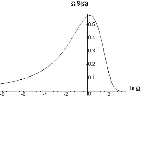
FIG. 1.: Limiting form of the distribution function for the rescaled logariphm of the conductivity.

REFERENCES

[1]Fractals and Disordered Systems, Ed. by A. Bunde, S.
Havlin (Springer Verlag, Berlin-Heidelberg-New-York, 1992).
[2] T. Nakayama, K. Yakubo and R. L. Orbach, Rev. Mod. Phys.,
66, 381, (1994).
[3] M. Ben-Chorin, F. Moller, F. Koch, W. Schirmacher and M.
Eberhard, Phys. Rev. B, 51, 2199 (1995).
[4] D. Cassi, S. Regina, Phys. Rev. Lett., 76, 2914, 1996.
[5] A.N. Samukhin, V.N. Prigodin, L. Jastrabík, Phys.
Rev. Lett, 78, 326, 1997.
[6] J. Tsukamoto, Adv. Phys., 41, 509 (1992).
[7] K. Araya, T. Micoh, T. Narahara, K. Akagi and H. Shirakawa,
Synth. Metals, 17, 247 (1987).
[8] Z. H. Wang, H. H. S. Javadi, A. Ray, A. J. MacDiarmid
and A. J. Epstein, Phys. Rev. B, 42, 5411 (1990).
[9] J. Joo, Z. Oblakowski, G. Du, J. P. Pouget, E. J. Oh, J.
M. Weisinger, Y. Min, A. G. MacDiarmid and A. J. Epstein: Phys. Rev. B, 49, 2977 (1994).
[10] L. P. Kadanoff, Ann. Phys. (N.Y.), 100, 359 (1976).
[11] C. Tsallis and A. C. N. de Magalhães, Phys. Repts., 268, 305 (1996).
[12] A. A .Migdal, Sov. Phys. JETP, 42; 413, 743 (1976).
[13] L. P. Kadanoff and A. Houghton, Phys. Rev. B, 11,
377 (1975).
[14] S. Kirkpatrick, Phys. Rev. B, 15, 1533 (1977).
[15] J-P. Normand and H. J. Herrmann, Int. J. Mod. Phys. C, to be
published.