Non–Equilibrium Dynamics of the Anderson Impurity Model

Abstract

The $M$–channel Anderson impurity model ($M=1,2$) is studied in the Kondo limit with a finite voltage bias applied to the conduction electron reservoirs. Using the Non–Crossing Approximation (NCA), we calculate the local spectral functions, the differential conductance, and susceptibility at non–zero bias for symmetric as well as asymmetric coupling of the impurity to the leads. We describe an effective procedure to solve the NCA integral equations which enables us to reach temperatures far below the Kondo scale. This allows us to study the scaling regime where the conductance depends on the bias only via a scaling function. Our results are applicable to both tunnel junctions and to point contacts. We present a general formula which allows one to go between the two cases of tunnel junctions and point contacts. Comparison is also made between the conformal field theory and the NCA conduction electron self-energies in the two channel case.

]

I Introduction

In recent years, the Kondo model and the Anderson impurity model in its Kondo limit have been investigated extensively by use of numerical renormalization group (NRG) calculations,[5, 6] the Bethe ansatz method,[7, 8] conformal field theory (CFT),[9] and auxiliary particle techniques. In this way a consistent theoretical understanding of the Kondo effect in equilibrium has emerged. In particular, the ground state of the system depends on the symmetry group of the conduction electron system: If the number of channels, $M$, is less than the level degeneracy, $N$, the screening of the local moment at energies below the Kondo scale, $T_{K}$, leads to a singlet Fermi liquid ground state with strongly renormalized Fermi liquid parameters. If, in contrast, $M\geq N$, the ground state is M–fold degenerate, leading to a non-vanishing entropy at zero temperature $T$ and a characteristic energy dependence of the density of states, obeying fractional power law below the Kondo scale. This is mirrored in an anomalous (non–Fermi liquid) behavior of the thermodynamics as well as transport properties[9].

On the other hand, there has been much less work on the non–equilibrium Kondo problem, where the electron distribution is not in local equilibrium about the Kondo impurity and linear response theory is no longer sufficient. Possible new effects in this situation include the breaking of time reversal symmetry and the appearance of a new energy scale like the charge transfer rate through a tunneling or point contact. The phenomena of tunneling through magnetic impurities has been explored since the 1960’s when zero bias anomalies (ZBA) were observed in metal-insulator-metal tunnel junctions.[10, 11] The origin of these zero bias anomalies was understood in terms of perturbative theories, [12] which captured the basic phenomena: a logarithmic temperature dependence and a Zeeman splitting of the ZBA peak in a finite magnetic field. Although the original theories were quite successful in fitting the data,[13] they were not able to get to what we now know as the low temperature strong coupling regime of the Kondo problem. In view of theoretical advances since that time, it is worthwhile to re-examine the non–equilibrium Kondo effect, particularly in the low temperature regime.

In addition, there have been a number of new and interesting realizations of the Kondo effect in non–equilibrium. With recent advances in sample fabrication, it has become possible to see a zero bias anomaly caused by a single Kondo impurity.[14] Even more intriguing is the observation of zero bias anomalies in point contacts that exhibit logarithmic temperature dependence at high temperatures and power law behavior at low temperatures but no Zeeman splitting in a magnetic field [15, 16, 17]. Such zero bias anomalies may be described by the two–channel Kondo model, where the ZBA is caused by electron assisted tunneling in two–level systems (TLS), although other descriptions have been proposed as well. [18]

In the 1980’s Zawadowski and Vladar [19] showed that if two-level-systems with sufficiently small energy splittings existed in metals, then one could observe a Kondo effect due to the electrons scattering off these TLS. In this case the TLS plays the role of a pseudo–spin. One state of the two-level-system may be regarded as pseudo–spin-up and the other as pseudo–spin-down. An electron scattering off the TLS can cause the pseudo-spin state of the TLS to change. The electron state also changes, e.g. its parity, in the process. This electron–assisted pseudo–spin–flip scattering plays the role of spin-flip scattering in the standard case of the magnetic Kondo effect. Detailed analysis, taking into account the different partial waves for scattering off the TLS shows that a Kondo effect is indeed generated by this electron–assisted tunneling. However, since the true electron spin is conserved in scattering from the TLS, there are two kinds or channels of electrons. Hence the the system will display the two–channel Kondo effect[20]. Level splitting and multi–electron scattering may disrupt the two–channel non–Fermi liquid behavior. The stability of the two–channel fixed point against these perturbations is currently a subject of investigation[19, 21, 22].

In recent years a number of techniques have been applied to the non–equilibrium Kondo problem: variational calculations,[23] perturbation theory,[24] equation of motion,[25] perturbative functional integral methods,[26] and exactly solvable points of the model.[27] One of the most powerful techniques in this context is the auxiliary boson technique[28, 29, 30]. It has two major advantages: (i) In its lowest order self–consistent approximation, the non–crossing approximation (NCA)[31, 32, 33], it yields an accurate quantitative description of the single–channel Anderson model in equilibrium[33, 34, 35] down to low temperatures, although it does not capture correctly the Fermi liquid regime. The NCA even describes the infrared dynamics of the two–channel model correctly as one approaches zero temperature. [36] (ii) The NCA is based on a standard self–consistent Feynman propagator expansion. Therefore, in contrast to exact solution methods, it need not rely on special symmetry properties which are not always realized in experiments. The formalism also allows for systematic improvements of the approximation.[37, 38, 39] Moreover, the NCA may be generalized for non–equilibrium cases in a straight–forward manner. This has been achieved recently for the single–channel Anderson model.[40, 41] However, the low temperature strong coupling regime of the model was not reached.

In this article we give a formulation of the NCA away from equilibrium which allows for a highly efficient numerical treatment, so that temperatures well inside the low energy scaling regime may be reached. In order to enable other researchers in this field to more readily apply this method to related problems we describe the numerical implementation of the formalism in some detail. Subsequently, we study a number of non-equilibrium properties of the single– and especially the two–channel Anderson model in the Kondo regime: (1) In linear response we study the conductance of the two channel model and the one channel model for different spin degeneracies. We use both tunnel junction and point contact geometries and discuss how to go continuously between the two. These results are compared to the bulk resistivity. (2) The nonlinear response is computed for the same Anderson models, and the scaling of the differential conductance at low temperatures and voltages is studied. (3) The NCA self-energies are compared to those obtained by conformal field theory. This sheds light on the question how far the equilibrium CFT results for the scaling function are applicable to non–equilibrium situations. (4) The effect of an asymmetry in the coupling of the impurity to the two leads is studied and shown to be consistent with asymmetries of ZBA’s observed experimentally. (5) Finally, we compute the effect of finite bias on the local (pseudo)spin susceptibility. Temperature and voltage scaling is verified below $T_{K}$, but large differences between the temperature and the voltage dependence are found outside of the scaling regime.

The paper is organized as follows: In section II the one– and two–channel Anderson models and their applicability to tunnel junctions and point contacts with defects are discussed. Section III contains the formulation of the problem within the NCA and discusses its validity for the single– and the two–channel case, respectively. An effective method for the solution of the NCA equations both for equilibrium and for static non–equilibrium is introduced. Section IV contains the results for the quantities mentioned above, which are discussed in comparison with equilibrium CFT solutions and experiments, where applicable. All the results are summarized in Section V.

II The SU(N)$\times$SU(M) Anderson impurity model out of equilibrium

A The model and physical realizations

The single–channel ($M=1$) and multi–channel ($M>1$) Kondo effects occur when a local $N$–fold degenerate degree of freedom, $\sigma=1,\dots,N$, is coupled via an exchange interaction to $M$ identical conduction electron bands, characterized by a continuous density of states and a Fermi surface. For example, the ordinary Kondo effect occurs when a magnetic impurity is coupled to conduction electrons via an exchange interaction. The impurity with spin $S$ plays the role of the $N=2S+1$ degenerate degrees of freedom, and there is only one flavor or channel of conduction electrons so $M=1$. There are other physical situations where there are $M$ bands of conduction electrons which are not scattering into each other. In this case one says that there are $M$ channels or flavors of electrons. For the $M$ channel Kondo effect, the channel or flavor degree of freedom, $\tau=1,\dots,M$, is assumed to be conserved by the exchange coupling.

Because of the non–canonical commutation relations of the spin algebra, this model is not easily accessible by standard field theoretic methods. Rather than work directly with the Kondo model, it is frequently more convenient to work with the corresponding Anderson model. Within the Anderson model, each of the possible spin or pseudo-spin states, $\sigma$, is represented by a fermionic particle. By convention the operator which creates a fermion in the local level $\sigma$ from a conduction electron in channel $\tau$ is denoted by $d_{\sigma\tau}^{{\dagger}}$. Since each of the d–states created by $d_{\sigma\tau}^{{\dagger}}$, represents a different (pseudo)spin state, only one of the states should be occupied at a time. In order to enforce this constraint, we use the auxiliary boson technique[28] and write $d_{\sigma\tau}^{{\dagger}}$ as $d^{{\dagger}}_{\sigma\tau}=f^{{\dagger}}_{\sigma}b_{\bar{\tau}}$, where $f_{\sigma}$ is a fermion operator and $b_{\tau}$ is a boson operator describing the unoccupied local d–level. The constraint is then written as the operator identity $Q=\sum_{\sigma}f^{{\dagger}}_{\sigma}f_{\sigma}+\sum_{\tau}b^{{\dagger}}_{\tau}b_{\tau}=1$. In terms of pseudo-fermion operators $f_{\sigma}$ and slave boson operators $b_{\bar{\tau}}$, the SU(N)$\times$SU(M) Anderson model is

$$H = \sum_{\vec{k},\sigma,\tau,\alpha}(\varepsilon_{\vec{k}}-eV_{\alpha})c^{\alpha\ {\dagger}}_{\vec{k}\sigma\tau}c^{\alpha}_{\vec{k}\sigma\tau}+\varepsilon_{d}\sum_{\sigma}f^{{\dagger}}_{\sigma}f_{\sigma}$$ (1)

$$+ \sum_{\vec{k},\sigma,\tau,\alpha}U_{\alpha}(f^{{\dagger}}_{\sigma}b_{\bar{\tau}}c^{\alpha}_{\vec{k}\sigma\tau}+h.c.),$$ (2)

where $f_{\sigma}$, ($\sigma=1,\dots N$) transforms according to SU(N) and $b_{\bar{\tau}}$, ($\bar{\tau}=1,\dots M$) transforms according to the adjoint representation of SU(M). The first term in Eq. (2) describes the conduction electron bands with kinetic energy $\varepsilon_{\vec{p}}$ offset by $-eV_{\alpha}$ due to an applied voltage. The index $\alpha$ is equal to $L$, $R$ for the left and the right reservoirs, respectively. Note that the two reservoirs do not constitute different scattering channels in the sense of the multi–channel model, since the reservoir index $\alpha$ is not conserved by the Kondo interaction. The second and third terms represent the energy of d–states and the hybridization term, respectively. The constraint term is not explicitly written in the Hamiltonian Eq. (2). Note that the local charge $Q$ commutes with the Hamiltonian.

As discussed in the introduction, there are a number of possible physical realizations of the one-channel non–equilibrium Kondo model: magnetic impurities in tunnel junctions, tunneling through charge traps, and possibly even tunneling through quantum dots. In each of these models the d-states introduced in the Anderson model have physical meaning. In the case of a transition metal magnetic impurities the d-states are literally the atomic d-states of the impurity. For a charge trap, the d-states are the electronic states for the two possible spin orientations of the trap. The two-channel model has been proposed as a possible scenario for the occurrence of non–Fermi liquid behavior in some heavy fermion compounds with cubic crystal symmetry.[35, 42, 43] In that case the occupied d–states correspond to the states of a low–lying non-magnetic doublet of the rare earth or actinide atoms, while the empty levels, described by $b_{\bar{\tau}}$, constitute an excited doublet of local orbitals[43].

On the other hand, for the physical realization in terms of two-level-systems, the empty states ($b_{\bar{\tau}}^{{\dagger}}$) do not have direct physical meaning. They are introduced as a construct in representing the pseudo–spins such that the channel quantum number $\tau$ is conserved by the Kondo interaction. Via a Schrieffer–Wolff transformation [44] one can show that the low energy physics of the Anderson model of Eq. (2) is the same as for the Kondo model in the limit when the occupation of the d-states $n_{d}$ approaches one. Thus, although we use the Anderson model, the results for the low energy physics are expected to be the same as for the Kondo model.

B The Non–crossing Approximation (NCA)

1 Validity of the NCA

In the present context we are interested in the Kondo regime of the Anderson model Eq. (2), where the low energy effective coupling $J_{\alpha}=|U_{\alpha}|^{2}/\varepsilon_{d}$ between the band electrons and the impurity is small, ${\cal N}(0)J_{\alpha}\ll 1$, with ${\cal N}(0)$ the band electron density of states per (pseudo–) spin and channel. The NCA is a self–consistent conserving perturbation expansion for the pseudo–fermion and slave boson self–energies to first order in ${\cal N}(0)J_{\alpha}$. Considering the inverse level degeneracy $1/N$ as an expansion parameter, the NCA includes all self–energy diagrams up to ${\cal O}(1/N)$. The self–energies are then made self–consistent by inserting the dressed slave particle propagators in the Feynman diagrams instead of the bare propagators.[30, 31, 32, 33] It is easiliy seen that this amounts to the summation of all self-energy diagrams without any propagator lines crossing each other, hence the name Non-crossing Approximation.

One may expect that the self–consistent perturbative approach is valid as long as the summation of higher orders in $J_{\alpha}$ or $1/N$ do not produce additional singularities of perturbation theory. It has recently been shown[37, 38, 45] that such a singularity does arise in the single–channel case ($M=1$, $N=2$) below the Kondo temperature $T_{K}$ due to the incipient formation of the singlet bound state between conduction electrons and the local impurity spin. However, around and above $T_{K}$ and in the Kondo limit of the two–channel model ($N=2$, $M=2$) even down to the lowest temperatures this singularity is not present[37]. Indeed, the NCA has been very successful in describing the single–channel Kondo model except for the appearance of spurious non–analytic behavior at temperatures far below $T_{K}$. The spurious low temperature properties are due to the fact that the NCA neglects vertex corrections responsible for restoring the Fermi liquid behavior of the single–channel model.[34, 37]. A qualitatively correct description was achieved[33, 34] for the wide temperature range from well below $T_{K}$ (but above the breakdown temperature of NCA) through the crossover region around $T_{K}$ up to the high temperature regime $T>T_{K}$. For the multi–channel problem, $M\geq N$, the complications of the appearance of a spin screened Fermi liquid fixed point are absent. For this case it has recently been shown[36] that the NCA does reproduce the exact[8, 9] low–frequency power law behavior of all physical properties involving the 4–point slave particle correlation functions, like the impurity spectral function $A_{d}$ and the susceptibilities, down zero temperature. Therefore, in the multi–channel case the NCA is a reliable approximation[46] for quantities involving $A_{d}$ (like the non–equilibrium conductance) and the susceptibilities, even at the lowest temperatures.

2 NCA in thermodynamic equilibrium

The slave boson perturbation expansion is initially formulated in the grand canonical ensemble, i.e.  in the enlarged Hilbert space of pseudo–fermion and slave boson degrees of freedom, with a single chemical potential $-\lambda$ for both pseudo–fermions and slave bosons. Therefore, standard diagram techniques are valid, including Wick’s theorem. In a second step, the exact projection of the equations onto the physical Hilbert space, $Q=1$, is performed[30, 33, 41]. For a brief review of the projection technique we refer the reader to appendix A.

The equations for the self–energies of the retarded Green functions of the pseudo-fermions, $G^{r}(\omega)=(\omega-\epsilon_{d}-\Sigma^{r}(\omega))^{-1}$, and the slave-bosons, $D^{r}(\omega)=(\omega-\Pi^{r}(\omega))^{-1}$, constrained to the physical subspace, read

$$\Sigma^{r}(\omega) = M\frac{\Gamma}{\pi}\int d\epsilon\bar{\cal N}(\omega-\epsilon)f(\epsilon-\omega)D^{r}(\epsilon)$$ (4)

$$\Pi^{r}(\omega) = N\frac{\Gamma}{\pi}\int d\epsilon\bar{\cal N}(\epsilon-\omega)f(\epsilon-\omega)G^{r}(\epsilon)\,\,\,,$$ (5)

where $\Gamma=\pi|U|^{2}{\cal N}(0)$, $\bar{\cal N}(\omega)={\cal N}(\omega)/{\cal N}(0)$ is the bare density of states of the band electrons, normalized to its value at the Fermi level, and $f(\omega)=1/(1+e^{\beta\omega})$ is the Fermi function. The real and imaginary parts of the self-energy are related via Kramers–Kroenig relations, e.g.

$$\mbox{Re}\Sigma^{r}(\omega)=\frac{1}{\pi}{\cal P}\int d\epsilon\frac{\mbox{Im}\Sigma^{r}(\epsilon)}{\epsilon-\omega}.$$ (6)

Taking the imaginary part of Eqs. (II B 2) and defining the spectral functions for the slave particles as,

$$A(\omega) = -\mbox{Im}G^{r}(\omega)/\pi=-\mbox{Im}\Sigma^{r}(\omega)\,|G^{r}(\omega)|^{2}/\pi$$ (7)

$$B(\omega) = -\mbox{Im}D^{r}(\omega)/\pi=-\mbox{Im}\Pi^{r}(\omega)\,|D^{r}(\omega)|^{2}/\pi$$ (8)

we arrive at the self–consistent equations

$$\frac{A(\omega)}{|G^{r}(\omega)|^{2}} = M\frac{\Gamma}{\pi}\int d\epsilon\bar{\cal N}(\omega-\epsilon)f(\epsilon-\omega)B(\epsilon)$$ (11)

$$\frac{B(\omega)}{|G^{r}(\omega)|^{2}} = N\frac{\Gamma}{\pi}\int d\epsilon\bar{\cal N}(\epsilon-\omega)f(\epsilon-\omega)A(\epsilon)\,.$$ (12)

Together with the Kramers-Kroenig relations, Eq. (6), Eqs. (II B 2) form a complete set of equations to determine the slave particle propagators. However, an additional difficulty arises in the construction of physical quantities from the auxiliary particle propagators. The local impurity propagator, $G_{d,\sigma\tau}(\tau-\tau^{\prime})=-\langle\hat{T}\{d_{d,\sigma\tau}(\tau)d_{d,\sigma\tau}^{{\dagger}}(\tau^{\prime})\}\rangle$, is given by the $f-b$ correlation function. Thus, its spectral function is calculated within NCA as[32]

$$A_{d}(\omega)=\frac{1}{Z}\int d\epsilon e^{-\beta\epsilon}\left[\,A(\epsilon+\omega)B(\epsilon)+A(\epsilon)B(\epsilon-\omega)\right],$$ (13)

where

$$Z=\int d\epsilon e^{-\beta\epsilon}[NA(\epsilon)+MB(\epsilon)]$$ (14)

is the canonical partition function of the impurity in the physical Hilbert space, $Q=1$ (see appendix A). The requirement that $Z$ be finite implies that the auxiliary particle spectral functions vanish exponentially below a threshold energy $E_{o}$.[31, 32] Above the threshold, the spectral functions show characteristic power law behavior originating[37] from the Anderson orthogonality catastrophe. In Eqs. (13), (14) the Boltzmann factor does not allow for a direct numerical evaluation of the integrand at negative $\epsilon$ if $\beta=1/k_{B}T$ is large. It is therefore necessary to absorb the Boltzmann factor in the spectral functions and find solutions for the functions

$$a(\omega)=e^{-\beta\omega}A(\omega)\,\,,\,\,\,\,\,b(\omega)=e^{-\beta\omega}B(\omega)\,\,.$$ (15)

Using $e^{\beta\omega}f(\omega)=f(-\omega)$, the equations determining $a(\omega)$ and $b(\omega)$ are easily found from Eqs. (II B 2):

$$\frac{a(\omega)}{|G^{r}(\omega)|^{2}}=M\frac{\Gamma}{\pi}\int d\epsilon\bar{\cal N}(\omega-\epsilon)f(\omega-\epsilon)b(\epsilon)$$ (17)

$$\frac{b(\omega)}{|G^{r}(\omega)|^{2}}=N\frac{\Gamma}{\pi}\int d\epsilon\bar{\cal N}(\epsilon-\omega)f(\omega-\epsilon)a(\epsilon)\,\,\,.$$ (18)

The equations for the impurity spectral function and the partition function then become

$$A_{d}(\omega)=\frac{1}{Z}\int d\epsilon\left[\,A(\epsilon+\omega)b(\epsilon)+a(\epsilon)B(\epsilon-\omega)\right]$$ (19)

$$Z=\int d\epsilon\left[Na(\epsilon)+Mb(\epsilon)\right]\,.$$ (20)

In view of the generalization to non–equilibrium, it is instructive to realize that the functions $a(\omega)$ and $b(\omega)$ are proportional to the Fourier transform of the lesser Green functions used in the Keldysh technique[47],

$$a(\omega) = \frac{i}{2\pi}G^{<}(\omega),\,\,\,\,\,G^{<}(t-t^{\prime})=-i\langle\,f^{{\dagger}}(t^{\prime})f(t)\,\rangle$$ (21)

$$b(\omega) = \frac{i}{2\pi}D^{<}(\omega),\,\,\,\,\,D^{<}(t-t^{\prime})=i\langle\,b^{{\dagger}}(t^{\prime})b(t)\rangle,$$ (22)

and contain information about the distribution functions of the slave particles. Henceforth we will call $a(\omega)$ and $b(\omega)$ the ‘lesser’ functions. Eqs. (II B 2), (II B 2) and (6) form a set of self–consistent equations which allow for the construction of the impurity spectral function $A_{d}$.

A significant simplification of the above procedure can be achieved by exploiting that in equilibrium the Eqs. (II B 2) and (II B 2) are not independent but linked to each other by Eq. (15). Hence, we define new functions $\tilde{A}(\omega)$ and $\tilde{B}(\omega)$ via[38]

$$f(-\omega)\tilde{A}(\omega)=A(\omega)\,\,,\,\,\,\,f(-\omega)\tilde{B}(\omega)=B(\omega).$$ (23)

By definition, $\tilde{A}(\omega)$ and $\tilde{B}(\omega)$ do not have threshold behavior, and the spectral functions as well as the lesser functions may easily be extracted from them, i. e. $a(\omega)=f(\omega)\tilde{A}(\omega)$, $B(\omega)=f(\omega)\tilde{B}(\omega)$. Inserting Eq. (23) into Eqs. (II B 2) one obtains the NCA equations for $\tilde{A}(\omega)$ and $\tilde{B}(\omega)$,

$$\frac{\tilde{A}(\omega)}{|G^{r}(\omega)|^{2}} = M\frac{\Gamma}{\pi}\int d\epsilon\bar{\cal N}(\omega-\epsilon)\frac{f(\epsilon-\omega))f(-\epsilon)}{f(-\omega)}\tilde{B}(\epsilon)$$ (25)

$$\frac{\tilde{B}(\omega)}{|G^{r}(\omega)|^{2}} = N\frac{\Gamma}{\pi}\int d\epsilon\bar{\cal N}(\epsilon-\omega)\frac{f(\epsilon-\omega)f(-\epsilon)}{f(-\omega)}\tilde{A}(\epsilon).$$ (26)

One can convince oneself that the statistical factors appearing in these equations are non–divergent in the zero temperature limit for all frequencies $\omega$, $\epsilon$. Thus, by solving the two Eqs. (II B 2) instead of the four Eqs. (II B 2), (II B 2), one saves a significant amount of integrations. The equations are solved numerically by iteration. After finding the solution at an elevated temperature, $T$ is gradually decreased. As the starting point of the iterations at any given $T$ we take the solution at the respective previous temperature value. In appendix A we describe an elegant and efficient implementation of the NCA equations which leads to a significant improvement in computational precision as well as speed. The proper setup of the discrete frequency meshes for the numerical integrations in the equilibrium and in the non–equilibrium case is dicussed in some detail in appendix B. In this way temperatures of 1/1000 $T_{K}$ and below may be reached without much effort. The solutions we obtained fulfill the exact sum rules

$$n_{d}\equiv N\int d \epsilon\,f(\epsilon)A_{d}(\epsilon)=N{\int}d\epsilon\,a(\epsilon)\equiv n_{f}$$ (27)

$$\int d \epsilon\,A_{d}(\epsilon)=1-(1-\frac{1}{N})n_{f}$$ (28)

typically to within 0.1% or better, where $n_{d}$ and $n_{f}$ are the occupation numbers of physical $d$–particles and pseudo–fermions in the impurity level, respectively.

An important quantity is the self–energy $\Sigma_{c}(\omega)$ of the conduction electrons due to scattering off the Kondo or Anderson impurities. In the limit of dilute impurity concentration $x\ll 1$, it is proportional to the bulk (linear response) resistivity of the system and determines the renormalized conduction electron density of states, which can be measured in tunneling experiments. Below we will calculate $\Sigma_{c}(\omega)$ within NCA in order to compare with the CFT prediction for the resistivity in equilibrium on one hand, and to compare the linear response result with the zero bias conductance calculated from a generalized Landauer–Büttiger formalism (see section III A) on the other hand.

$\Sigma_{c}(\omega)$ is defined via the impurity averaged conduction electron Green function in momentum space, $G_{c\,{\bf k}}(\omega)=[\omega-\varepsilon_{\bf k}-\Sigma_{c}(\omega)]^{-1}$. In the dilute limit and for pure s–wave scattering, $\Sigma_{c}(\omega)$ is momentum independent,

$$\Sigma_{c}(\omega)=xt(\omega)\,$$ (29)

where $t(\omega)$ is the local $T$–matrix for scattering off a single impurity. According to the Hamiltonian, Eq. (2), $t(\omega)$ is given exactly in terms the local $d$–particle propagator and reads, e.g. for scattering across the junction ($L\rightarrow R$),

$$t(\omega)=U_{R}U_{L}^{*}G_{d}(\omega)\,.$$ (30)

C NCA for static non–equilibrium

If we apply a finite bias $V$, the system is no longer in equilibrium. We cannot expect the simple relation Eq. (15) between the lesser and the spectral functions to hold in this case. Therefore, the trick with introducing the functions $\tilde{A}$ and $\tilde{B}$ cannot be performed. Rather, the NCA equations have to be derived by means of standard non–equilibrium Green function techniques,[41, 47, 48] and one has to solve the equivalent of Eqs. (II B 2) and (II B 2) for the non–equilibrium case without any further simplification. Defining in analogy to the equilibrium case $\Gamma_{L,R}=\pi|U_{L,R}|^{2}{\cal N}(0)$, the NCA equations for steady state non–equilibrium are

$$\frac{A(\omega)}{|G^{r}(\omega)|^{2}}=\frac{M}{\pi}\int d\epsilon B(\epsilon)$$ (32)

$$\times\sum_{\alpha=L,R}\left[\Gamma_{\alpha}\bar{\cal N}(\omega-\epsilon+\mu_{\alpha})f(\epsilon-\omega-\mu_{\alpha})\right]$$ (33)

$$\frac{B(\omega)}{|G^{r}(\omega)|^{2}}=\frac{N}{\pi}\int d\epsilon A(\epsilon)$$ (34)

$$\times\sum_{\alpha=L,R}\left[\Gamma_{\alpha}\bar{\cal N}(\epsilon-\omega-\mu_{\alpha})f(\epsilon-\omega-\mu_{\alpha})\right]$$ (35)

$$\frac{a(\omega)}{|G^{r}(\omega)|^{2}}=\frac{M}{\pi}\int d\epsilon\,b(\epsilon)$$ (37)

$$\times\sum_{\alpha=L,R}\left[\Gamma_{\alpha}\bar{\cal N}(\omega-\epsilon+\mu_{\alpha})f(\omega-\epsilon+\mu_{\alpha})\right]$$ (38)

$$\frac{b(\omega)}{|G^{r}(\omega)|^{2}}=\frac{N}{\pi}\int d\epsilon\,a(\epsilon)$$ (39)

$$\times\sum_{\alpha=L,R}\left[\Gamma_{\alpha}\bar{\cal N}(\epsilon-\omega-\mu_{\alpha})f(\omega-\epsilon+\mu_{\alpha})\right].$$ (40)

If the density of states ${\cal N}(\omega)$ were a constant, the only difference between the equilibrium and the non–equilibrium NCA equations would be the replacement of the Fermi function by an effective distribution function $F_{eff}$ given by

$$F_{eff}(\epsilon)=\frac{\Gamma_{L}}{\Gamma_{tot}}f(\epsilon-\mu_{L})+\frac{\Gamma_{R}}{\Gamma_{tot}}f(\epsilon-\mu_{R}),$$ (41)

where $\Gamma_{tot}=\Gamma_{L}+\Gamma_{R}$. Since our density of states is a Gaussian with a width much larger than all the other energy scales, $|\epsilon_{d}|,\,\Gamma_{tot},\,T_{K}$, this is in fact the only significant modification of the NCA equations. Numerically, the most crucial modification concerns the integration mesh. The proper choice of integration meshes is central to the success of the iteration and is discussed in Appendix B.

III Current formulae, conductance and susceptibilities

A Current formulae and conductance

For the case of tunneling through a Kondo impurity, the current is directly related to the impurity Green functions. In particular, the current in the left or in the right lead is given[24, 40] by a generalized Landauer–Büttiger formula,

$$I_{L}(V) = -N\frac{e}{\hbar}\Gamma_{L}\int d\omega\bar{\cal N}(\omega-\mu_{L})$$ (43)

$$\times \left[G_{d}^{<}(\omega)-A_{d}(\omega)f(\omega-\mu_{L})\right]$$ (44)

$$I_{R}(V) = N\frac{e}{\hbar}\Gamma_{R}\int d\omega\bar{\cal N}(\omega-\mu_{R})$$ (45)

$$\times \left[G_{d}^{<}(\omega)-A_{d}(\omega)f(\omega-\mu_{R})\right],$$ (46)

where $G_{d}^{<}$ is the lesser Green function of the impurity. It is obtained from the pseudo–fermion and slave boson Green functions via

$$G_{d}^{<}(\omega)=\frac{1}{Z}\int d\epsilon\,a(\epsilon)B(\epsilon-\omega)\,.$$ (47)

Making use of current conservation, $I_{L}=I_{R}$, and taking the wide band limit, where ${\cal N}(\omega)$ is taken to be a constant, the current may be expressed solely in terms of the impurity spectral function

$$I(V) = N\frac{e}{\hbar}\frac{2\Gamma_{L}\Gamma_{R}}{\Gamma_{L}+\Gamma_{R}}\int d\omega A_{d}(\omega)$$ (48)

$$\times [f(\omega-\mu_{L})-f(\omega-\mu_{R})].$$ (49)

The NCA is a conserving approximation.[41] Therefore, the currents computed for the left and the right leads should be the same when evaluated numerically. We have checked the current conservation within NCA and found that the two currents agree to within 0.5%, which sets a limit to the uncertainty for the average current, $I(V)=(I_{L}+I_{R})/2$.

In order to obtain the differential conductance, $G(V)=dI(V)/dV$, we perform the numerical derivative $(I(V_{1})-I(V_{2}))/(V_{1}-V_{2})$, and take it as the value of $G(V)$ $V=(V_{1}+V_{2})/2$. The numerical error involved in this procedure could be reduced to as little as 2%. The zero bias conductance (ZBC) is the special case of the above equations in the limit of vanishing applied voltage $V\rightarrow 0$. The ZBC for a tunnel junction is thus

$$G(0,T)=N\frac{e^{2}}{\hbar}\frac{2\Gamma_{L}\Gamma_{R}}{\Gamma_{L}+\Gamma_{R}}\int d\omega\left(-\frac{\partial f(\omega)}{\partial\omega}\right)A_{d}(\omega).$$ (50)

It will be useful to compare this to the linear response bulk resistivity for a small density of impurities in a metal. The resistivity, $\rho$, is related to the impurity spectral function via [33]

$$1/\rho=const\int d\omega\left(-\frac{\partial f(\omega)}{\partial\omega}\right)\tau(\omega),$$ (51)

where the impurity scattering rate is $\tau^{-1}(\omega)=xU_{L}U_{R}^{*}A_{d}(\omega)$. The impurity concentration is denoted by $x$.

Most of our calculations were done with symmetric couplings, $\Gamma_{L}=\Gamma_{R}$. However, this is not necessarily the case in an experimental situation, especially for tunnel junctions. When an Anderson impurity is placed inside a tunneling barrier of thickness $d$, the tunneling matrix element $U_{\alpha}$ depends exponentially on the distance $z$ of the impurity from the surface of the the barrier. Also, the bare energy level $\varepsilon_{d}$ of the impurity will be shifted due to the approximately linear in $z$ voltage drop inside the barrier. In order to investigate the consequences on the non–equilibrium conductance, we also performed evaluations with asymmetric couplings. For simplcity, and in order to keep the total coupling $\Gamma_{tot}=\Gamma_{L}+\Gamma_{R}$ constant, we assume a linear dependence of the $\Gamma_{\alpha}$’s on $z$ of the form $\Gamma_{L}=\Gamma_{tot}(1-z/d)\,,\,\,\,\Gamma_{R}=\Gamma_{tot}z/d$. We also modify $\epsilon_{d}$ according to $\epsilon_{d}(V)=\epsilon_{d}+(V/2)(1-2z/d)$. The latter modification turns out to be insignificant as long as $V|\epsilon_{d}|$.

B Tunnel junctions vs. point contacts

The above formulae for the currents and conductances are valid in a tunnel junction geometry where the current must flow through the impurity. In a point contact the two leads are joined by a small constriction. A current $I_{o}$ will flow through the constriction without the impurity being present. In fact, the impurity will impede the current due to additional scattering in the vicinity of the constriction. The question arises whether the effect of an impurity in a point contact is the same in magnitude but opposite in sign. In Appendix C we derive a general formula for the conductance which allows one to go continuously between a clean point contact and a tunnel junction. In the limit of a clean point contact, where the transmission probabilities are close to unity, we find that the change in the conductance due to an impurity in a point contact has the same form as for a tunnel junction, except for a change in sign. Thus, in clean samples the results for the current calculated for the tunnel junction apply for point contacts as well, if one subtracts out the background current, $I_{o}$. If $I_{o}$ is ohmic, the conductance $G(V)$ is shifted by the constant $dI_{o}/dV$. Aside from this shift and sign difference, the conductance signals of a tunnel junction and a clean point contact will be the same.

C Susceptibilities

The impurity contribution to the dynamic (pseudo-) spin susceptibility is calculated using the standard formulae [32, 33] from the lesser and the spectral function of the pseudo-fermions. The formula for the imaginary part reads

$$\mbox{Im}\chi(\omega)=\frac{1}{Z}\int\frac{d\epsilon}{\pi}\left[\,A(\epsilon+\omega)a(\epsilon)-a(\epsilon)A(\epsilon-\omega)\right]\,\,\,.$$ (52)

The real part can be obtained by means of a Kramers–Kroenig relation:

$$\mbox{Re}\chi(\omega)=\frac{1}{\pi}{\cal P}\int d\epsilon\frac{\mbox{Im}\chi(\epsilon)}{\epsilon-\omega}.$$ (53)

The static susceptibility $\chi_{o}=\chi(\omega=0)$ follows directly from this equation. Note that in the two–channel Anderson model as possibly realized in TLS’s, this susceptibility is not the magnetic susceptibility. Rather, it is probed by a field coupling to the impurity pseudospin, e.g. a crystal field breaking the degeneracy of the TLS.

IV Results

A Conductance for one– and two–channel models with symmetric couplings

Using the formulae discussed in the previous section, we now present the results obtained from the numerical evaluation of the bulk resistivity and of the conductance for symmetric couplings. For the evaluations a Gaussian conduction electron density of states ${\cal N}(\omega)$ with half width $D$ was used. All calculations were done in the Kondo regime for the set of parameters $\varepsilon_{d}=-0.67D$, $\Gamma_{L}=\Gamma_{R}=0.15D$. In order to make the most direct comparison to experiment, the results for the two–channel case have been computed for a point contact, and the results for the one channel case have been computed for a tunnel junction, except for Fig. 4 where we compare the scaling behavior of the nonlinear conductance for the one– and two–channel models.

1 Linear response conductance and resistivity

The low temperature limit of the linear response conductance shows power law behavior in temperature. The exponent is determined by the symmetry of the underlying Kondo model. As explained in the discussion of the NCA, we expect to get quantitatively correct behavior for the two channel model, but not for the one channel case. In Fig. 1 we show the zero bias correction to the conductance $G(0,T)$ for a two channel Kondo impurity ($N=M=2$) in a point contact. The zero bias conductance does show the expected[9] $T^{1/2}$ dependence at low $T$. Deviations from this power law start at about 1/4 $T_{K}$, where the Kondo temperature $T_{K}$ is determined from the data as the width at half maximum of the zero bias impurity spectral function, $A_{d}$, at the lowest calculated $T$ (see Fig. 12). The slope of the $T^{1/2}$ behavior defines a constant $B_{\Sigma}$:

FIG. 1.: Temperature dependence of the zero bias conductance for the two–channel model ($M=2$, $N=2$) in a point contact. The zero bias conductance has $T^{1/2}$ dependence for $T<T_{K}/4$. This can be used to roughly extract $T_{K}$ from the experimental data. $B_{\Sigma}$ (compare Eq. (27)) is a material dependent constant which has been divided out. Therefore, the slope of the low $T$ fit (dashed line) is equal to unity.

$$G(0,T)-G(0,0)=B_{\Sigma}T^{1/2},$$ (54)

which we will use below in interpreting the nonlinear conductance.

On the other hand, for the one channel case ($M=1,N=2$) one expects $T^{2}$ dependence because of the Fermi liquid behavior at low temperatures. As shown in Fig. 2 for a tunnel junction, the NCA as a large N expansion is not able to reproduce this power law for $N=2$ at temperatures below $T_{K}$. Increasing $N$ to $N=4$ and $N=6$, the ZBC develops a hump as a function of

FIG. 2.: Zero bias conductance for tunneling through a single–channel Anderson impurity ($M=1$, $N=2$) vs. temperature. The conductance for a clean point contact in the presence of a single–channel Kondi impurity would be obtained by subtraction of this curve from a (constant) background conductance. The graph for $N=2$ shows an almost linear $T$ dependence at low $T$ whereas the curves for spin degeneracy $N=4$ and $N=6$ show non–monotonic behavior. The humps are due to the fact that the Kondo peak of the spectral function $A_{d}(\omega)$ is shifted away from the Fermi energy $\epsilon_{F}$ by about $T_{K}$. For $T>T_{K}$ all the curves fall like log$(T/T_{K})$ for approximately one decade.

temperature. This peak is due to the fact that the Kondo resonance is shifted away from the Fermi level for $N>2$. Although we know of no experimental evidence for such humps in zero bias anomalies, similar humps have be seen in the magnetic susceptibilities of these systems.[33] Note that for $N=6$, a $T^{2}$ behavior seems to appear at temperatures below the hump. The temperature range shown here is above the breakdown temperature of NCA, below which a fractional power law $G(0,T)-G(0.0)\propto-T^{M/(M+N)}$ would appear.

For a bulk Kondo system it is impossible to measure the zero bias conductance of single impurities. Instead, one measures the linear response resistivity, $\rho$. In Fig. 3 we show the impurity contribution to the resistivity for one channel impurities with $N=2,4,6$. Only the $N=6$ curve shows a convex dependence on $T$. In fact, $\rho$ seems to behave like $(1-const(T/T_{K})^{2})$ at the temperatures shown, consistent with a Fermi liquid. [33] For $N=2$ there is no convex temperature dependence even down to $T=0.02T_{K}$. Figures 2 and 3 also serve to illustrate that the zero bias conductance and the bulk resistivity for the same kind of Kondo impurities do not necessarily have the same temperature dependence.

FIG. 3.: Bulk resistivity vs. temperature for the $M=1$ channel model, $N=2,4,6$. Of the three curves only $N=6$ has a clear convex shape and falls roughly like $T^{2}$ at low $T$. The $N=2$ graph again shows almost linear $T$ dependence. Note that the humps in the conductance for $N=4$ and $N=6$ are not present in the bulk resistivity $\rho$.

2 Nonlinear conductance

Recently, it has been shown [49] that the two–channel model exhibits scaling of the nonlinear conductance $G(V,T)$ as a function of bias $V$ and $T$ of the form [16]

$$G(V,T)-G(0,T)=B_{\Sigma}T^{\eta}H(A\frac{eV}{k_{B}T})\,\,.$$ (55)

Here, $H$ is a universal scaling function which satisfies $H(0)=0$ and $H(x)\propto x^{\eta}$ for $x\gg 1$, and $A$, $B_{\Sigma}$ are non-universal constants. The exponent $\eta$ is 1/2 for the two–channel model. This scaling ansatz is motivated by

FIG. 4.: Scaling plots of the conductance of point contacts in the presence of (a) a two–channel impurity ($M=N=2$) and (b) a one–channel impurity ($M=1$, $N=2$). With $\Gamma_{L}=\Gamma_{R}$ and $B_{\Sigma}$ determined from the zero bias conductance (compare Eq. (27)), there are no adjustable parameters. There are two regimes in these plots. For $(eV/k_{B}T)^{\eta}<1.5$ the curves collapse onto a single curve and the rescaled conductance is proportional to $(eV/k_{B}T)^{2}$. For larger $(eV/k_{B}T)^{\eta}$ the rescaled conductance is linear on these plots. There are substantial corrections to scaling even at $T$ small compared to $T_{K}$. At even larger biases this linear behavior rounds off, indicating the breakdown of scaling. The temperatures are given in units of the respective $T_{K}$ for the two– and the one–channel case.

the scaling of the conduction electron self–energy in the variables frequency $\omega$ and temperature $T$ as obtained by CFT in equilibrium.[9] Scaling behavior is well known[5] to be present also in the equilibrium properties of the single–channel model ($M=1$, $N=2$). Hence, in the case $M=1$ one may expect a scaling form of the non–equilibrium conductance similar to Eq. (55) as well, however with Fermi liquid exponent $\eta=2$.

In order to examine whether the scaling ansatz is correct, the rescaled conductance is plotted as a function of $(eV/k_{B}T)^{\eta}$. The conductance curves for different $T$ should collapse onto a single curve with a linear part for not too large and not too small arguments: Very large $V$ or $T$ would drive the system out of the scaling regime. A collapse indeed occurs for low bias $V<T$. However, for larger bias the slope of the linear part shows $T$ dependence (see Ref. [[49]] for more details). This shows that there are significant $T$–dependent corrections to scaling, indicating that finite bias $V$ and finite temperature $T$ are not equivalent as far as scaling is concerned, although both parameters have qualitatively similar effects on the conductance.

Figs. 4 (a) and (b) show the scaling plots for the cases $M=2$ and $M=1$, respectively, with $N=2$ in both cases. Whereas the two–channel case shows the behavior described above with the expected exponent $\eta=1/2$, the NCA does not give the correct exponent for the single–channel model. In fact, the data show approximate scaling, however, the exponent $\eta$ extracted from the NCA data appears to be equal to unity rather than 2. This seems to reflect the dominant linear temperature dependence of the ZBC that the NCA produces in this case. This shortcoming is another consequence of the negligence of singular vertex corrections within the NCA.

B Self–energy scaling and comparison to CFT

Two possible origins for the above mentioned finite–$T$ corrections to scaling at low temperatures $T$ are: (i) The non–equilibrium state brings about terms in the electron self-energy which break scaling of the form given by CFT, and (ii) the deviations from scaling in equilibrium at finite $T$ have large coefficients, restricting the scaling regime to $T\ll T_{K}$.

Recently, it has been shown for the single–channel model[27] that in non–equilibrium the conductance indeed has terms which explicitly break the scaling behavior. Though the coefficients of these terms are small, scaling in the ordinary sense is clearly violated, i.e. at temperatures well below a crossover temperature ($T_{K}$) not all corrections to scaling vanish. It is quite possible that the two–channel Kondo model behaves in an analogous fashion.

Within the NCA we here investigate case (ii) by examination of the behavior of the self-energies in equilibrium. As mentioned above, within CFT[9] the retarded conduction electron self–energy $\Sigma_{c}(\omega,T)$ of the two–channel particle–hole symmetric Kondo model is found to obey scaling of the form

$$\mbox{Im}\Sigma_{c}(\omega,T)-\mbox{Im}\Sigma_{c}(0,T)=bT^{1/2}H(\frac{\hbar\omega}{k_{B}T})\,\,,$$ (56)

where $H$ is again a universal scaling function of the kind introduced above ($\eta=1/2$). The constant, $b$, is non-universal. Within CFT the sign of $b$ the sign depends on whether one is on the weak coupling or the strong coupling side of the (intermediate coupling) fixed point[9]. The NCA calculation is on the weak coupling side and yields a positive constant $b$ (see below), in agreement with CFT. However, a direct quantitative comparison with CFT is less straight–forward because the model used in the CFT calculation is particle–hole (p–h) symmetric, while ours is not: The local level $\epsilon_{d}$ has a finite position

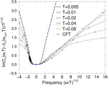
FIG. 5.: Scaling plot for the imaginary part of the retarded conduction electron self-energy for a small concentration ($x=1\%$) of the $M=2$ channel Anderson impurities in a noninteracting metal. Temperatures are given in units of $T_{K}$. $\mbox{Im}\Sigma_{c}$ has a minimum that is shifted to positive frequencies due to finite temperature effects. The data are scaled with respect to the point ($\omega_{min},\mbox{Im}\Sigma(\omega_{min})$. For frequencies below $\omega_{min}$ the self-energy behaves like $(\omega/T)^{1/2}$ and scales well up to frequencies of the order of $T_{K}$. However, for positive frequencies the self-energy is strongly temperature dependent and scaling is less perfect. The parameters of the CFT prediction for the particle–hole symmetric Kondo model (dashed line) have been adjusted so that the slope for negative arguments matches that of the lowest temperature NCA curve.

below the Fermi level, while the on–site repulsion is taken to be infinite. The scaling plot Fig. 5 shows a very strong asymmetry about the point $\omega=0$. The temperature dependence is also substantial. The parameters of the CFT curve (dashed line) have been adjusted so that the slope for the linear part in $(\omega/T)^{1/2}$ for negative frequencies matches the slope of the lowest $T$ NCA curve. The asymmetry of the conduction electron self–energy may be traced back to the p–h asymmetry of our model. P–h asymmetry may very well be present in the experimental systems[16]. However, no or only small asymmetries are seen in the measurements of the nonlinear conductance. This is presumably because in the expression for the nonlinear current, Eq. (49), the frequency is integrated over both positive and negative values, $-V/2\leq\omega\leq+V/2$, thus averaging out the asymmetry. This conjecture is supported by our calculation of the conduction electron self–energy (Fig. 5), which displays strong p–h symmetry, and the non–linear conductance[49] (Fig. 4), which is almost p–h symmetric.

Finally, in the Anderson model we also consider the impurity electron self-energy $\Sigma_{d}(\omega,T)$. It can easily be computed from the d–Green function. The two physical self-energies $\Sigma_{d}(\omega,T)$ and $\Sigma_{c}(\omega,T)$ are nonlinearly related via Eqs. (29), (30) for a system of dilute impurities in an equilibrium situation. It should be noted that the nonlinear conductance is directly related to the spectral function $A_{d}(\omega)$ via Eq. 49. We first examine whether the impurity self-energy $\Sigma_{d}(\omega,T)$ shows scaling behavior in equilibrium in the variables $\omega$ and $T$. The imaginary

FIG. 6.: Scaling plot for the imaginary part of the impurity electron self-energy for the $M=2$ channel Anderson model. Temperatures are given in units of $T_{K}$. For different temperatures $T$, $\mbox{Im}(\Sigma_{d}(\omega,T)-\mbox{Im}\Sigma_{d}(0,T))/(cT^{1/2})$ is plotted versus the square root of the scaled frequency, $(\omega/T)^{1/2}$. The constant $c$ depends on details of the model. The left parts of the curves ($\omega<0$) obey the anticipated square root behavior and scale very well for $|\omega|\ll T_{K}$. For $\omega/T>0$ the NCA curves show a strong $T$–dependence even for $T\ll T_{K}$. This is a possible origin of the $T$ dependent slopes of the nonlinear conductance curves in Fig. 5. However, for modestly large frequencies, e.g. $\omega/T<4$ the lowest $T$ curves seem to follow square root behavior, too. The general asymmetry of the self-energy is a consequence of the particle–hole asymmetry of the Anderson model considered here.

part of the retarded impurity self-energy is negative by causality and its absolute value shows a peak at the Fermi level. In Fig. 6, we plot $(Im\Sigma_{d}(\omega,T)-Im\Sigma_{d}(0,T))/(cT^{1/2})$ vs. $(\omega/T)^{1/2}$ for different temperatures $T$. The constant $c$ is positive and depends on the parameters of the model. Obviously, the left parts of the curves ($\omega<0$) obey scaling very well. For arguments of $(\omega/T)^{1/2}$ outside the scaling regime $\omega,T<T_{K}$ the curves bend, and the self-energies grow roughly logarithmically (not shown in the figure). In contrast, the $\omega/T>0$ parts of the NCA–curves show a strong $T$–dependence even for $T\ll T_{K}$, again a consequence of p–h asymmetry. Nevertheless, at negative frequencies scaling with the correct power law is established over a wide range of the scaling argument $(\omega/T)^{1/2}$, as long as $\omega,T<T_{K}$, even though $\omega$ can be much larger than $T$. It is very plausible that this scaling is reflected in the scaling of the nonlinear conductance in the arguments bias and temperature as observed in experiment[16] and our numerical evaluation.[49] Furthermore, the deviations from scaling at positive frequencies could be another reason for the observed finite $T$–corrections to scaling of the conductance.[49]

C Conductance with asymmetric couplings

Up to this point we have taken the couplings of the impurity to the conduction bands to be equal, $\Gamma_{L}=\Gamma_{R}$. As mentioned before, especially for a tunnel junction there is no reason why this should be the case. The NCA–Eqs. (II C), (II C) are not symmetric in the couplings, that is $\Gamma_{L}\leftrightarrow\Gamma_{R}$ is not a symmetry of the equations. This suggests that the differential conductance signals are not symmetric about zero bias if $\Gamma_{L}\neq\Gamma_{R}$. Indeed, the Onsager relations for a two terminal measurement only apply to the linear response regime. For nonlinear response there is no simple relation between $I(V)$ and $I(-V)$. However, interchanging both $\Gamma_{L}\leftrightarrow\Gamma_{R}$ and $V\leftrightarrow-V$ is a symmetry. It is therefore enough to show only the conductances for $\Gamma_{L}>1/2$. The curves with $\Gamma_{L}<1/2$ can be obtained from the $\Gamma_{L}>1/2$ ones by reflection about the y-axis.

An example of such asymmetric conductance curves is shown in Fig. 7. The data is for the two–channel model, but the qualitative aspects of asymmetry does not depend on the channel number. The constant $B_{\Sigma}$ is dependent on the asymmetry, but has been divided out for better comparison of the curves. The asymmetry is pronounced even for moderate deviations from symmetric coupling. Asymmetric conductance vs. voltage curves similar to those shown in Fig. 7 have been observed in Ta-I-Al tunnel junctions,[13] where they were plotted as an odd in voltage contribution to the differential conductance.

FIG. 7.: Nonlinear conductance for the $M=2$ channel case for asymmetric coupling, $\Gamma_{L}\neq\Gamma_{R}=1-\Gamma_{L}$. As expected from the asymmetry of the NCA equations (16) and (17), the conductance signals show a quite strong asymmetry about zero bias even for moderate differences in the couplings. Asymmetries in the conductance have been observed in metal–insulator–metal tunnel junctions.

D Dynamic and static susceptibility for the two channel model

Finally, we also show results for the static and dynamic susceptibilities with and without finite bias. Although it is unlikely that one will be able to measure the susceptibility for a single impurity, the susceptibility is one of the clearest measures of the screening of the impurity by electrons. All data shown below is for the two channel

FIG. 8.: Imaginary part of the dynamic susceptibility ${\rm Im}\chi(\omega)$ (arb. units) for the $M=2$ channel Anderson model in equilibrium ($V=0$). Temperatures are given in units of $T_{K}$. For $T\rightarrow 0$, $\chi(\omega)$ behaves as $\mbox{Im}\chi(\omega)\simeq c_{1}\mbox{sign}(\omega)[1-c_{2}\sqrt{|\omega/T_{K}|}]$, in agreement with exact results for the two–channel case. This is in contrast to the exact linear behavior in the $M=1$ channel model.

model. The results for the usual Kondo model show different power laws, but the general effect of the finite bias is the same.

In equilibrium, in the zero temperature limit, the dynamic susceptibility defined in Eq. (52) is given by a step function of the form [36]

$$\mbox{Im}\chi(\omega)=c_{1}\mbox{sign}(\omega)\biggl{[}1-c_{2}\sqrt{\bigl{|}\frac{\omega}{T_{K}}\bigr{|}}+\mbox{\ldots}\biggr{]}\,\,\,.$$ (57)

The NCA approaches this behavior as the temperature is reduced. At finite temperature, the step is broadened, as shown in Fig. 8, with the extrema located at values

FIG. 9.: Static susceptibility $\chi_{o}$ (arb. units) vs. temperature at zero and at finite bias $V$ for $M=2$, $N=2$. In equilibrium, $\chi_{o}$ shows the characteristic, expected logarithmic divergence as $T$ approaches zero for the two–channel model. Out of equilibrium, this divergence is cut off at a temperature corresponding to the bias $V$. The inset shows that $\chi_{o}$ falls with $T^{2}$ below this cutoff. For high temperatures $T\gg T_{K}$, $\chi_{o}$ falls like $1/T$ (Curie–Weiss law).

FIG. 10.: Static susceptibility $\chi_{o}$ (arb. units) vs. bias $V$ at various temperatures $T$ for $M=2$, $N=2$. Temperatures are given in units of $T_{K}$. $\chi_{o}$ has a very similar dependence on $V$ and $T$ as long as $V,T<T_{K}$ (scaling regime). $\chi_{o}$ drops like $V^{2}$ for $T\buildrel<\over{\sim}0.1T_{K}$ and like log$(V)$ around $T_{K}$. However, for large $V\gg T_{K}$, $\chi_{o}$ falls less rapidly with $V$ than with $T$, see Fig. 11.

which grow roughly with $T^{1/2}$. The real part follows by a Kramers-Kroenig relation and diverges logarithmically for $\omega\rightarrow 0$, again cut off at finite $T$. As a consequence, the static susceptibility $\chi_{o}={\rm Re}\chi(\omega=0)$ diverges logarithmically as $T$ approaches zero in agreement with non–Fermi liquid behavior, as has been predicted before. [8, 9, 36] This logarithmic divergence is well reproduced by the NCA technique, see Fig. 9

Out of equilibrium, the finite bias serves as another low energy cutoff, but in a nontrivial manner. If we look at the extrema of the imaginary part of the susceptibility

FIG. 11.: Product of the static susceptibility $\chi_{o}$ and temperature $T$ (bias $V$) vs. $T$ ($V$) on a semi–logarithmic scale for $M=2$, $N=2$. The $T$ dependence shows saturation at high temperatures and therefore implies the Curie law, $\chi_{o}\propto 1/T$. However, the $V$ dependence is linear at large bias, implying that $\chi_{o}$ falls less rapidly with $V$ than with $T$, $\chi_{o}\propto\mbox{log}(V)/V$. The y–axis units are such that a “free pseudo–spin” would correspond to a constant value of 1/2 (Curie–behavior at large temperatures).

at low temperature but finite bias ($V>T$) we find that they are located at smaller absolute values than at the corresponding temperature. The logarithmic divergence of the Re$\chi(\omega)$ is cut off at about $V$, so that the static susceptibility does not diverge logarithmically as $T\rightarrow 0$ anymore. Instead, it approaches a ($V$–dependent) finite value with a quadratic $T$–dependence (see inset of Fig. 9). However, this does not signal the return of Fermi liquid behavior for $T<V$, since we still have $\sqrt{V/T}$ behavior of the conductance for $V$ well below $T_{K}$. Fig. 9 shows the $T$–dependence of $\chi_{o}$ for $V=1/10T_{K}$.

FIG. 12.: The impurity spectral function $A_{d}(\omega)$ for the $M=2$ channel, $N=2$ Anderson model for various biases $V$. The half width at half maximum of the zero bias spectral function (solid line) is a measure of $T_{K}$. As the voltage is increased to $eV=k_{B}T_{K}$ the Kondo resonance is reduced (dash-dotted line). At very large bias the resonance shows a shoulder and eventually splits into two peaks. Increasing the temperature would wash out the peak splitting and restore a single, much less pronounced peak.

Similar behavior (i.e. quadratic in $V$ for low $V$, logarithmic for $T<V<T_{K}$) is observed for the $V$–dependence of the static susceptibility (see Fig. 10); however, there is a difference in the dependence on $T$ and $V$ in the regime $T_{K}<T,V$ and $T,V<\Gamma_{tot}$. For large $T>T_{K}$ at zero bias the static susceptibility behaves like $1/T$, indicating Curie-Weiss behavior. However, for large $V$ at low temperature $\chi_{o}$ falls less rapidly. The difference becomes obvious if we plot $V\chi_{o}$ vs. $\log(V)$ and $T\chi_{o}$ vs. $\log(T)$ as shown in Fig. 11. Whereas the $T$-dependence saturates, indicating the free moment at high temperatures the $V$-dependence shows linear behavior, leading to $\chi_{o}\sim b\log(V)/V$. This stresses again the different consequences of rising $T$ and $V$ once one has left the scaling regime $T,V<T_{K}$. The latter becomes most obvious if we look at the impurity spectral function $A_{d}(\omega)$ for various values of the bias, see Fig. 12. For zero bias and low temperatures there is a sharp resonance with width $T_{K}$ (solid line). Increasing the temperature above $T_{K}$ the peak would broaden at the expense of its height (not shown). In contrast, if we keep the temperature low, $T\ll T_{K}$, and increase the bias, the resonance first develops a shoulder and then splits into two much broader but distinguished peaks (see $eV=10k_{B}T$ and $20k_{B}T$). Increasing the temperature would eventually wash out the peak splitting and restore a single, though much less pronounced peak. This difference in behavior at large $T$ vs. large $V$ is the reason for the breakdown of scaling of the conductance for $T$ or $V$ larger than $T_{K}$ and the different behavior of the susceptibility at large arguments (Fig. 11).

V Conclusion

In conclusion, we have described in detail the analytical foundations and the numerical implementation of the NCA integral equations for the one– and two–channel Anderson model out of equilibrium. Our algorithms enabled us to reach lower temperatures than previously obtained, allowing us to study the physics deep inside the scaling regime of the two–channel model.

In linear response, we computed the conductance for tunnel junctions and point contacts as well as the bulk resistivity. The two–channel data for both properties show $T^{1/2}$ behavior in agreement with results obtained by other methods. For the single–channel model and $N=2$ we find dominantly linear behavior below $T_{K}$. For $N=6$ the bulk resistivity drops with $T^{2}$ (Fermi liquid behavior) at the lowest temperatures considered in this work; however, the tunnel junction conductance rises with $T^{2}$, reaches a maximum below the Kondo temperature $T_{K}$ and then falls off logarithmically at higher $T$. This “hump” is associated with the fact that the Kondo peak of the impurity spectral function is shifted away from the Fermi level for values of $N>2$.

If we turn on a finite bias $V$, the Kondo peak of the impurity spectral function first diminishes in height and broadens, then splits into two peaks located at the energies of the two Fermi levels of the leads at a bias of about $10T_{K}$. The non–equilibrium conductance is again consistent with linear behavior in the regime $T<V<T_{K}$ for the single–channel case with $M=1$, $N=2$. Therefore, we can plot the conductance as a function of $eV/k_{B}T$ and achieve scaling for modest bias $V$. Whether similar scaling of the conductance but with argument $(eV/k_{B}T)^{2}$ can exist for the case $N=6$ is yet to be determined. The tunnel junction conductance falls with $V^{2}$ for bias $V<T_{K}$. This is in stark contrast to the hump in the $T$–dependence of the zero bias conductance. If at all, scaling seems possible only for temperatures well below the temperature where the hump occurs. The two channel data show scaling with respect to the argument $(eV/k_{B}T)^{1/2}$ consistent with conductance measurements on clean point contacts. It has to be pointed out, though, that the scaling at non–zero bias in the two–channel as well as in the single–channel model is only approximate. Finite $T$ corrections are observed in the numerical data (and also in the experimental data) for temperatures down to about $1/100\,T_{K}$. This indicates that finite bias $V$ and finite temperature $T$ are not equivalent, although they have qualitatively similar effects on the conductance. The scaling of the conduction electron self-energy turns out to be worse than that of the nonlinear conductance. This may be traced back to the lack of particle–hole symmetry of our model, which leads to asymmetries in the self-energy even at the lowest temperature. Additionally, there are also strong temperature dependent corrections to the square root behavior.

If we allow for asymmetric couplings to the left and right Fermi seas, we observe conductance signals which are asymmetric about zero bias. Such features have been seen in experiments on metal-insulator-metal tunnel junctions.

Finally, we also calculated the dynamic and static (pseudo–) spin susceptibility and discussed the modifications due to a finite bias by example of the two channel model. The dynamic susceptibility approaches a finite step at $\omega=0$ as $T\rightarrow 0$, leading to a logarithmic divergence of the static susceptibility in agreement with CFT results. A finite bias cuts off this logarithmic divergence. In a very similar fashion the temperature cuts off the divergence as the bias is vanishing. Differences in the bias and temperature dependence of the static susceptibility appear at high bias and temperature outside of the scaling regime.

It is a pleasure to acknowledge discussions with V. Ambegaokar, R. Buhrman, J. von Delft, D. Ralph, S. Upadhyay, L. Borkowski P. Hirschfeld, K. Ingersent, A. Ludwig, A. Schiller, and M. Jarrell. This work was supported by NSF grant DMR-9357474, the U.F. D.S.R., the NHMFL (M.H.H., S.H.), by NSF grant DMR-9407245, the German DFG through SFB 195 and by a Feodor Lynen Fellowship of the Alexander v. Humboldt Foundation (J.K). Part of the work of J.K. was performed at LASSP, Cornell University.

A Numerical implementation of the NCA equations

Below we briefly review the slave boson projection technique and describe an implementation which allows for a highly accurate as well as efficient numerical treatment of the singularities of the spectral functions, which arise from the projection.

The exact projection of the expectation value of any operator $\hat{\cal O}$ onto the physical subspace, $Q=1$, is achieved by first taking the statistical average in the grand canonical (GC) ensemble with a chemical potential $-\lambda$ for both fermions $f$ and bosons $b$, and then differentiating w.r.t. the fugacity $\zeta={\rm exp}(-\beta\lambda)$ and taking the limit $\lambda\rightarrow\infty$,

$$\langle\hat{\cal O}\rangle_{C} = \lim_{\lambda\rightarrow\infty}\frac{\frac{{\rm d}}{{\rm d}\zeta}tr[\hat{\cal O}{\rm e}^{-\beta(H+\lambda Q)}]}{\frac{{\rm d}}{{\rm d}\zeta}tr[{\rm e}^{-\beta(H+\lambda Q)}]}$$ (A1)

$$= \frac{\lim_{\lambda\rightarrow\infty}\langle\hat{\cal O}\rangle_{GC}{\rm e}^{\beta\lambda}}{\lim_{\lambda\rightarrow\infty}\langle Q\rangle_{GC}{\rm e}^{\beta\lambda}}$$ (A2)

Note that in this expression the factor $Q$ arising from the differentiation ${\rm d}/{\rm d}\zeta$ in the numerator may be dropped for any operator ${\cal O}$ whose expectation value in the subspace $Q=0$ vanishes (like, e.g., ${\cal O}=d_{\sigma\tau}(t)d^{{\dagger}}_{\sigma\tau}(t^{\prime})$ or any other physically observable operator on the impurity site). The canonical (C) partition function is given by

$$Z = \lim_{\lambda\rightarrow\infty}\left[{\rm e}^{\beta\lambda}\langle Q\rangle_{GC}(\lambda)\right]\,Z_{Q=0}$$ (A3)

$$= Z_{Q=0}\,\int d\epsilon{\rm e}^{-\beta\epsilon}(NA(\epsilon)+MB(\epsilon))\,,$$ (A4)

where $Z_{Q=0}$ is the partition function in the subspace $Q=0$.

The integrals involved in the NCA equations are difficult to compute because of the singular threshold structure[32] of $A(\omega)$, $B(\omega)$, where the position of the threshold energy $E_{o}$ is a priori not known. In order to make the numerical evaluations tractable, we apply a time t dependent $U(1)$ gauge transformation simultaneously to the $f$ and $b$ particles according to $f\rightarrow{\rm exp}(i\lambda_{o}t)f$, $b\rightarrow{\rm exp}(i\lambda_{o}t)b$. This transformation is a symmetry of the Anderson model and amounts to a shift of the slave particle energy or chemical potential by $\lambda_{o}$, $\omega\rightarrow\omega+\lambda_{o}$. Note that this shift does not affect any physical properties, as seen explicitly, e.g., from Eq. (19). After this energy shift, the spectral and lesser functions appearing in the NCA equations read

$$A_{\lambda_{o}}(\omega) = \frac{\mbox{Im}\Sigma^{r}(\omega)}{(\omega-\epsilon_{d}+\lambda_{o}-\mbox{Re}\Sigma^{r}(\omega))^{2}+(\mbox{Im}\Sigma^{r}(\omega))^{2}}$$ (A6)

$$B_{\lambda_{o}}(\omega) = \frac{\mbox{Im}\Pi^{r}(\omega)}{(\omega+\lambda_{o}-\mbox{Re}\Pi^{r}(\omega))^{2}+(\mbox{Im}\Pi^{r}(\omega))^{2}}$$ (A7)

$$a_{\lambda_{o}}(\omega) = \frac{\Sigma^{<}(\omega)}{(\omega-\epsilon_{d}+\lambda_{o}-\mbox{Re}\Sigma^{r}(\omega))^{2}+(\mbox{Im}\Sigma^{r}(\omega))^{2}}$$ (A9)

$$b_{\lambda_{o}}(\omega) = \frac{\Pi^{<}(\omega)}{(\omega+\lambda_{o}-\mbox{Re}\Pi^{r}(\omega))^{2}+(\mbox{Im}\Pi^{r}(\omega))^{2}}\,\,\,.$$ (A10)

In particular, we now have from Eq. (A4)

$$\frac{Z(\lambda_{o})}{Z_{Q=0}}={\rm e}^{-\beta\lambda_{o}}\int d\epsilon{\rm e}^{-\beta\epsilon}(NA(\epsilon)+MB(\epsilon))\,,$$ (A11)

The crucial point about making the numerics efficient is that $\lambda_{o}$ is determined in each iteration such that the integral in Eq. (A11) is equal to unity[38, 34]. This definition of $\lambda_{o}$ forces the zero of the auxiliary particle energy to coincide with the threshold energy, $E_{o}=0$ in each iteration step. Thus, it enables us to define fixed frequency meshes, which do not change from iteration to iteration and at the same time resolve the singular behavior very well, as described in appendix B. The procedure described above leads to a substantial gain in precision and significantly improves the convergence of the iterations, even though the equation determining $\lambda_{o}$ must be solved during each iteration.

From Eq. (A11) and the definition of the impurity contribution to the free energy, $F_{imp}(T)$, ${\rm exp}(-\beta F_{imp})=Z(T)/Z_{Q=0}(T)$, it is seen that $\lambda_{o}$ determined in the above way is just equal to $F_{imp}$. This provides a convenient way of calculating $F_{imp}(T)$ directly from the auxiliary particle Green functions.

B Integration meshes for equilibrium and non-equilibrium NCA

The various features of the auxiliary particle as well as the physical spectral functions are charcterized by energy scales, which differ by several orders of magnitude. These energy scales are the conduction band width $D$, the localized level $\epsilon_{d}$, and the dynamically generated Kondo scale, $T_{K}$, which is typically of order $10^{-4}D$. Moreover, because of the $T=0$, $V=0$ threshold divergence of the auxiliary particle spectral functions, the sharpest features have a width given by the temperature, which can be of the order of $10^{-7}D$. In non–equilibrium, the bias $V$ appears as an additional scale. In the numerical solution of the NCA equations, discrete, non–equidistant intregration meshes must be set up such that all the features at the various energy scales are well resolved.

These meshes can be generated by mapping the grid points $x_{i}$ of an equidistant mesh onto the non–equidistant frequency points $\omega_{i}$ by means of an appropriately chosen function $h(x)$. In the regions where the very sharp features of the spectral functions and the Fermi function appear, i.e. near $\omega=0$ and $\omega=\pm V/2$, respectively, we will use a logarithmicly dense mesh. On the other hand, in order to resolve the relatively broad peak centered around the local level $\varepsilon_{d}$, the substitution $\omega_{i}=\varepsilon_{d}+c\tan(x_{i})$ will be used.

In general, the entire interval of integration is composed of $L$ meshes $\{x^{l}_{i}\}$, $i=1\dots n_{l}$, $l=1\dots L$. We map these meshes onto the nonuniform frequency meshes $\{\omega^{l}_{i}\}$ via

$$\omega_{i}^{l}=h^{l}(x^{l}_{i}),\,\,\,\,\,\,\,\,i=1\ldots n^{l}.$$ (B1)

We can now rewrite the integration of an arbitrary function $k(\omega)$ as an integration over the “equidistant” variables $\{x_{i}^{l}\}$:

$$\int_{-\infty}^{\infty} d\omega k(\omega)=\sum_{l}\int_{a_{l}}^{b_{l}}dx\frac{\partial h^{l}(x)}{\partial x}k(h(x))$$ (B2)

$$\simeq \sum_{l}{\Delta x^{l}}\left(\sum_{i=2}^{n_{l}-1}\left[\frac{\partial h^{l}}{\partial x^{l}}(x^{l}_{i})k(h(x^{l}_{i}))\right]\right.$$ (B3)

$$+ \left.\frac{1}{2}\left[\frac{\partial h^{l}}{\partial x^{l}}(x^{l}_{1})k(h(x^{l}_{1}))+\frac{\partial h^{l}}{\partial x^{l}}(x^{l}_{n_{l}})k(h(x^{l}_{n_{l}}))\right]\right).$$ (B4)

The $a^{l}=\omega^{l}_{1},b^{l}=\omega^{l}_{n_{l}}$ are the limits of integration of the different regions of the frequency–axis. To cover the whole axis we must have $a^{l+1}=b^{l}$. In equilibrium, we can get by with four regions: $[-\infty,-\omega_{I}),\,[-\omega_{I},0=\epsilon_{F}),\,[0,\omega_{I}),\,[\omega_{I},\infty]$ , where $\omega_{I}$ is an interface frequency where two regions of the mesh are matched. ($|\epsilon_{d}|-\Gamma>\omega_{I}>>T_{K}$). By choosing the functions $h^{l}(x^{l})$ as $\varepsilon_{d}+c_{1}\tan(x^{l})$ in the regions with large absolute frequency and as $c_{2}\exp(x^{l})$ in the regions $|\omega|<\omega_{I}$ we create large mesh point spacings far from $\epsilon_{F}$ and exponentially small spacings (“logarithmic” mesh) at $\epsilon_{F}=0$. Proper adjustment of constants in the $h^{l}$’s is required. The frequency mesh point spacing near $\omega=0$ should be at least 10 times smaller than $T$ (and/or $V$ out of equilibrium). Crucial for the success of this procedure is the introduction of $\lambda_{o}$ (see Appendix A) in the iteration procedure. $\lambda_{o}$ shifts the peaks of the slave particle functions to the neighborhood of $\omega=0$ in each iteration step. This allows to define a fixed frequency grid, which leads to a significant increase in computational speed and precision.

Out of equilibrium the distribution function is a double step function with steps at $\pm V/2$. It turns out that in the Kondo limit the slave boson spectral and lesser functions show broadened peaks at about the same frequencies. However, the pseudo–fermion functions behave differently. They do not split, but have a single peak somewhere between the Fermi level and $V/2$ that shifts not linearly with $V$. To cope with such behavior we wish to have good resolution at $\pm V/2$ and at $\epsilon_{F}$. (The latter one is to improve the resolution at the location of the peak of the pseudo-fermion functions. Unfortunately, we do not know how this location will move with increasing $V$) . To achieve this we let the logarithmic mesh end at $\pm V/2$ coming from larger/smaller frequencies and choose the spacing in between according to the sum of two tanh–functions which have their zero shifted to $\pm V/4$, respectively. We have to choose parameters of these functions, so that the mesh spacings at the crucial energies is small enough to resolve all features of the integrand. These parameters depend on the bias $V$. They have to be calculated before the mesh is ’set up’ whenever we change the potential from one run to the next. However, once the mesh is set, we do not have to change it anymore during the iterations, because of the same reasons as in equilibrium.

The typical total number of integration points used is 200 and 250 for equilibrium and out of equilibrium, respectively. Out of equilibrium we need about 50 points more for the ‘inner’ region between $\pm V/2$ at moderate bias $V<20T_{K}$. For higher bias we have to introduce more points in the inner region. Convergence is achieved within 100 - 200 iterations. The CPU time to obtain a converged solution on a typical workstation is below 1 minute for the equilibrium case, and of the order of minutes for non–equilibrium.

C General formula for the conductance

In this appendix we derive Eq. (49) for the current through a constriction with an impurity. We proceed in three stages. First, we introduce our scattering state notation and review the noninteracting case. Next, we derive a general formula for scattering from an interacting impurity. This is valid for point contacts, tunnel junctions, and anything in between. Finally, we specialize to the case of a clean point contact.

The geometry we consider consists of perfect left ($L$) and right ($R$) leads connected by a central region where there is scattering. The scattering states, $\psi({\bf x})$, are eigenstates of the noninteracting problem. They are labeled by their incoming wave vectors, ${\bf k}$, where $k_{z}>0$ corresponds to a right moving wave and $k_{z}<0$ corresponds to a left moving wave, where $z$ is the direction along the length of the leads. For example, a state moving from left to right ($k_{z}>0$) has the asymptotic form for $z\gg 0$ of

$$\psi_{\bf k}({\bf x})=\sum_{{\bf k}_{\perp}^{\prime}}t_{{\bf k}^{\prime}{\bf k}}^{RL}\,\sqrt{|v_{z}/v_{z}^{\prime}|}\,e^{i|k^{\prime}_{z}|z}\,\varphi_{{\bf k}_{\perp}^{\prime}}({\bf x}_{\perp})$$ (C1)

and for $z\ll 0$ of

$$\psi_{\bf k}({\bf x}) = e^{i|k_{z}|z}\,\varphi_{{\bf k}_{\perp}}({\bf x}_{\perp})$$ (C2)

$$+ \sum_{{\bf k}_{\perp}^{\prime}}r_{{\bf k}^{\prime}{\bf k}}^{L}\,\sqrt{|v_{z}/v_{z}^{\prime}|}\,e^{-i|k^{\prime}_{z}|z}\,\varphi_{{\bf k}_{\perp}^{\prime}}({\bf x}_{\perp})$$ (C3)

The transverse modes, $\varphi_{{\bf k}_{\perp}}({\bf x}_{\perp})$, in Eqs. (C1) and (C2) are chosen to have unit normalization, and $v_{z}=k_{z}/m$ is the velocity along the length of the leads. It is also understood that the energy of the incident and transmitted waves are the same, $\epsilon_{{\bf k}_{\perp}}+\epsilon_{k_{z}}=\epsilon_{{\bf k}^{\prime}_{\perp}}+\epsilon_{k^{\prime}_{z}}$.

The current for both the interacting and the noninteracting case may be expressed as a cross-sectional integral of the ‘lesser’ Green function:

$$I=\int\frac{d\omega}{2\pi}\int d^{2}x_{\perp}\left(\frac{\nabla_{z}-\nabla_{z^{\prime}}}{2mi}\right)g_{<}({\bf x},{\bf x}^{\prime};\omega)\Big{|}_{{\bf x}={\bf x}^{\prime}}.$$ (C4)

For the noninteracting case, this Green function may be written in terms of the scattering states as

$$g_{<}^{o}(x,x^{\prime};\omega)=\int\frac{dk_{z}}{2\pi}\sum_{{\bf k}_{\perp}}2\pi\delta(\omega-E_{\bf k})\psi_{\bf k}({\bf x})\psi_{\bf k}^{*}({\bf x}^{\prime})f_{\bf k}(\omega),$$ (C5)

where $f_{\bf k}(\omega)$ is a Fermi function at chemical potential $\mu_{L}$ for $k_{z}>0$ and at $\mu_{R}$ for $k_{z}<0$. We will usually refer to these Fermi functions as $f_{L}(\omega)$ and $f_{R}(\omega)$, respectively. Using the asymptotic expressions of Eqs. (C1) and (C2) for the the right moving scattering states and the similar ones for the left moving states, Eqs. (C4) and (C5) lead to the usual Landauer formula for the conductance:

$$I=\int\frac{dE_{k}}{2\pi}\sum_{{\bf k}_{\perp}{\bf k}^{\prime}_{\perp}}|t^{RL}_{{\bf k}^{\prime}{\bf k}}|^{2}(f_{L}(E_{k})-f_{R}(E_{k})).$$ (C6)

We now add an impurity which includes an interacting term to the Hamiltonian. The coupling of the impurity, denoted by 0, to the electrons is given by

$$H^{\prime}=\int\frac{dk_{z}}{2\pi}\sum_{{\bf k}_{\perp}}W_{\bf k}c_{0}^{{\dagger}}c_{\bf k}+W_{\bf k}^{*}c_{\bf k}^{{\dagger}}c_{0},$$ (C7)

where ${\bf k}$ refers to the scattering state of incoming wave vector ${\bf k}$, not a plane wave state. In Eq. (C7) and in the previous equations we have not included spin. The entire derivation presented here follows through in the presence of a spin (or other) index so long as the self-energy is diagonal in that index. This is the case for the Anderson model used in this paper. In order to simplify the notation, we shall proceed without spin and at the end quote the final result when the electron spin is included.

Using Dyson’s equation one can express all of the Green functions for the full system, $g$, in terms of the noninteracting Green functions, $g^{o}$, and the full Green function at the impurity, $g(0,0)$. In particular the Green function $g_{<}({\bf k},{\bf k^{\prime}})$, which is used to compute the current, is given by

$$g_{<}({\bf k},{\bf k}^{\prime}) = 2\pi\delta(k_{z}-k_{z}^{\prime})\delta_{{\bf k}_{\perp}{\bf k}_{\perp}^{\prime}}g_{<}^{o}({\bf k})$$ (C8)

$$+ g_{<}^{o}({\bf k})W_{\bf k}^{*}g_{a}(0,0)W_{{\bf k}^{\prime}}g^{o}_{a}({\bf k}^{\prime})$$ (C9)

$$+ g_{r}^{o}({\bf k})W_{\bf k}^{*}g_{<}(0,0)W_{{\bf k}^{\prime}}g^{o}_{a}({\bf k}^{\prime})$$ (C10)

$$+ g_{r}^{o}({\bf k})W_{\bf k}^{*}g_{r}(0,0)W_{{\bf k}^{\prime}}g^{o}_{<}({\bf k}^{\prime}).$$ (C11)

In Eq. (C10) all Green functions have the same energy, $\omega$. The self-energy $\sigma$ contains the many body interaction at the impurity site. Equation (C10) is converted to real space using

$$g_{r}({\bf x},0)=\int\frac{dk_{z}}{2\pi}\sum_{{\bf k}_{\perp}}\psi_{\bf k}({\bf x})g_{r}({\bf k},0),$$ (C12)

and the similar relation for the advanced Green function. The result for the real space $g_{<}$ is

$$g_{<}({\bf x},{\bf x}^{\prime}) = g_{r}({\bf x},0)\,\sigma_{<}\,g_{a}(0,{\bf x}^{\prime})$$ (C13)

$$+ \int\frac{dk_{z}^{\prime\prime}}{2\pi}\sum_{{\bf k}_{\perp}^{\prime\prime}}\left\{\psi_{{\bf k}^{\prime\prime}}({\bf x})+g_{r}({\bf x},0)W_{{\bf k}^{\prime\prime}}\right\}$$ (C14)

$$\times g_{<}^{o}({\bf k}^{\prime\prime})\,\left\{\psi_{{\bf k}^{\prime\prime}}^{*}({\bf x^{\prime}})+W_{{\bf k}^{\prime\prime}}^{*}g_{a}(0,{\bf x}^{\prime})\right\}.$$ (C15)

As for the noninteracting case, we wish to evaluate the current far into the left and right leads. To do this we need the the asymptotic form of the scattering states (Eqs. (C1) and (C2)) and the asymptotic form of the retarded and advanced Green functions, $g_{r(a)}({\bf x},0)$, which we define as

$$\frac{g_{r}({\bf x},0)}{g_{r}(0,0)}=\sum_{{\bf k}_{\perp}}t^{R(L)}_{\bf k}\,\varphi_{{\bf k}_{\perp}}({\bf x}_{\perp})\,e^{+(-)i|k_{z}|z}\Big{|}_{E_{k}=\omega}.$$ (C16)

Substituting Eq. (C13) into Eq. (C4) for the current, then yields

$$I_{R} = \sum_{{\bf k}_{\perp},{\bf k}_{\perp}^{\prime\prime}}\int\frac{d\omega}{2\pi}|t^{RL}_{{\bf k}{\bf k}^{\prime\prime}}+t^{R}_{{\bf k}}g_{r}(0,0)W_{{\bf k}^{\prime\prime}}|^{2}f_{L}(\omega)$$ (C17)

$$+ \sum_{{\bf k}_{\perp},{\bf k}_{\perp}^{\prime\prime}}\int\frac{d\omega}{2\pi}(|r^{R}_{{\bf k}{\bf k}^{\prime\prime}}+t^{R}_{{\bf k}}g_{r}(0,0)W_{{\bf k}^{\prime\prime}}|^{2}-\delta_{{\bf k}_{\perp}{\bf k}_{\perp}^{\prime\prime}})f_{R}(\omega)$$ (C18)

$$+ \sum_{{\bf k}_{\perp}}\int\frac{d\omega}{2\pi}v_{z}^{\prime\prime}|t^{R}_{{\bf k}}g_{r}(0,0)|^{2}\sigma_{<}(\omega)$$ (C19)

$$I_{L} = -\sum_{{\bf k}_{\perp},{\bf k}_{\perp}^{\prime\prime}}\int\frac{d\omega}{2\pi}|t^{LR}_{{\bf k}{\bf k}^{\prime\prime}}+t^{L}_{{\bf k}}g_{r}(0,0)W_{{\bf k}^{\prime\prime}}|^{2}f_{R}(\omega)$$ (C20)

$$- \sum_{{\bf k}_{\perp},{\bf k}_{\perp}^{\prime\prime}}\int\frac{d\omega}{2\pi}(|r^{L}_{{\bf k}{\bf k}^{\prime\prime}}+t^{L}_{{\bf k}}g_{r}(0,0)W_{{\bf k}^{\prime\prime}}|^{2}-\delta_{{\bf k}_{\perp}{\bf k}_{\perp}^{\prime\prime}})f_{L}(\omega)$$ (C21)

$$- \sum_{{\bf k}_{\perp}}\int\frac{d\omega}{2\pi}|v_{z}^{\prime\prime}||t^{L}_{{\bf k}}g_{r}(0,0)|^{2}\sigma_{<}(\omega)$$ (C22)

Eqs. (C17) and (C20) are our most general expressions for the current. It is useful to compare them to those for the noninteracting case (Eq. (C6)). Without the terms involving $\sigma_{<}$, equations (C17) and (C20) have exactly the same structure as the noninteracting current. The effect of the impurity is to change the transmission probability for electrons coming from the left or the right. The $\sigma_{<}$ contains the “scattering-out” of an electron from the impurity state. This is a new feature of the interacting problem.

Equations (C17) and (C20) are valid for an arbitrary scattering potential, including both the tunnel junction case and the clean point contact case. We model the clean point contact case by a perfect wire. The wire will have a conductance equal to $e^{2}/h$ times the number of channels at the Fermi energy. The transmission and reflection probabilities for this case are 1 and 0:

$$\delta_{{\bf k_{\perp}},{\bf k_{\perp}^{\prime\prime}}} = t^{RL}_{{\bf k},{\bf k^{\prime\prime}}}=t^{LR}_{{\bf k},{\bf k^{\prime\prime}}}$$ (C23)

$$0 = r^{R}_{{\bf k},{\bf k^{\prime\prime}}}=r^{L}_{{\bf k},{\bf k^{\prime\prime}}}.$$ (C24)

In this perfect wire case the scattering states are plane waves. The impurity is placed at position, ${\bf x}={\bf a}$, and the overlap matrix elements are

$$W_{\bf k}=W^{L(R)}\frac{e^{ik\cdot a}}{\sqrt{{\cal A}}},$$ (C25)

where ${\cal A}$ is the cross-sectional area of the wire. As in Eqs. (C1) and (C2), the $L$ here refers to scattering states which start on the left, $k_{z}>0$, and $R$ refers to those which start on the right, $k_{z}<0$. The distinction between left and right moving is a probably unphysical here; however, it is useful to make contact to the tunnel junction case. Eq. (C25) implies that

$$t^{R(L)}_{\bf k}=\frac{W^{L(R)}e^{-ik\cdot a}}{\sqrt{{\cal A}}}\frac{1}{i|v_{z}|}.$$ (C26)

Finally, we define the scattering rate of state ${\bf k}$ from the impurity as

$$\Gamma^{A}_{\bf k}=\frac{|W^{A}|^{2}}{{\cal A}}\int\frac{dk_{z}}{2\pi}\pi\delta(\omega-\epsilon_{{\bf k}_{\perp}}-\epsilon_{k_{z}})=\frac{1}{2}\frac{1}{|v_{z}|}\frac{|W^{A}|^{2}}{{\cal A}},$$ (C27)

where the integral is done either over $k_{z}>0$ or $k_{z}<0$ for $A=L,\,R$, respectively. Current conservation requires that $I_{L}=I_{R}$ so in computing our final result for the current we can take any linear combination of $I_{L}$ and $I_{R}$ which is convenient:

$$I = \frac{|W^{L}|^{2}}{|W^{L}|^{2}+|W^{R}|^{2}}I_{L}+\frac{|W^{R}|^{2}}{|W^{L}|^{2}+|W^{R}|^{2}}I_{R}$$ (C28)

$$= \sum_{{\bf k}_{\perp}}\int\frac{d\omega}{2\pi}(f_{L}(\omega)-f_{R}(\omega))$$ (C29)

$$- \int{d\omega}\sum_{{\bf k}_{\perp}}\frac{2\Gamma_{\bf k}^{L}\Gamma_{\bf k}^{R}}{\Gamma_{\bf k}^{L}+\Gamma_{\bf k}^{R}}A_{d}(\omega)(f_{L}(\omega)-f_{R}(\omega)),$$ (C30)

where $A_{d}(\omega)=-\mbox{Im}g_{r}(0,0)/\pi$ is the impurity spectral function.

This is our final result for the number current. The first term gives the Sharvin point contact conductance. The second term is the correction to the current due to the presence of the impurity. The expression is the same as for a tunnel junction,[24, 40] except the sign is reversed. The correction to the current once one includes the electron spin is

$$\delta I=-\int{d\omega}\sum_{{\bf k}_{\perp},s}\frac{2\Gamma_{{\bf k},s}^{L}\Gamma_{{\bf k},s}^{R}}{\Gamma_{{\bf k},s}^{L}+\Gamma_{{\bf k},s}^{R}}A_{d,s}(\omega)(f_{L}(\omega)-f_{R}(\omega)),$$ (C31)

where the only change from Eq. (C29) is that there is a sum over the spin, $s$. If we assume a constant density of states and no spin dependence of the matrix elements, we obtain the expression Eq. (49), except for the difference in sign between the tunnel junction and point contact case. Note that in Eq. (49) the $\Gamma_{L}$ and $\Gamma_{R}$ are defined with the density of states divided out.

REFERENCES

- [1] [∗] Present address: Department of Physics, University of Cincinnati, Cincinnati, Ohio 45221.
- [2] E-mail: hettler@physics.uc.edu
- [3] [†] E-mail: kroha@tkm.physik.uni-karlsruhe.de
- [4] [‡] E-mail: selman@phys.ufl.edu
- [5] K. G. Wilson, Rev. Mod. Phys. 47, 773 (1975); H. R. Krishna–murthy, J. W. Wilkins and K. G. Wilson, Phys. Rev. B 21, 1003, (1980); ibid. 1044 (1980).
- [6] H. O. Frota and L. N. Oliveira, Phys. Rev. B 33, 7871 (1986).
- [7] N. Andrei, Phys. Rev. Lett. 45, 379 (1980); P. B. Wiegmann, J. Phys. C 14, 1463 (1981); N. Kawakami and A. Okiji, Phys. Lett. A 86, 483 (1981).
- [8] P. B. Wiegmann and A. M. Tsvelik, JETP Lett. 38, 591 (1983); N. Andrei and C. Destri, Phys. Rev. Lett. 52, 364 (1984).
- [9] A. W. W. Ludwig and I. Affleck, Phys. Rev. Lett. 67, 3160 (1991); I. Affleck and A. A. W. Ludwig, Phys. Rev. B 48, 7297 (1993).
- [10] A. F. G. Wyatt, Phys. Rev. Lett. 13, 401 (1964); R. A. Logan and J. M. Rowell, ibid. 13, 404 (1964).
- [11] D. J. Lythall and A. F. G. Wyatt, Phys. Rev. Lett. 20, 1361 (1968); L. Y. L. Shen and J. M. Rowell, Phys. Rev. 165, 566 (1968).
- [12] J. Appelbaum, Phys. Rev. Lett. 17, 91 (1966); P. W. Anderson, ibid. 17, 95 (1966). J. A. Appelbaum, Phys. Rev. 154, 633 (1967).
- [13] J. A. Appelbaum and L. Y. L. Shen, Phys. Rev. B 5, 544 (1972).
- [14] D. C. Ralph and R. A. Buhrman, Phys. Rev. Lett. 72, 3401 (1994).
- [15] D. C. Ralph and R. A. Buhrman, Phys. Rev. Lett. 69, 2118 (1992).
- [16] D. C. Ralph, A. W. W. Ludwig, J. v. Delft, and R. A. Buhrman, Phys. Rev. Lett. 72, 1064 (1994).
- [17] S. K. Upadhyay, R. N. Louie and R. A. Buhrman, to be published (1997).
- [18] N. Wingreen, Y. Meir and B. L. Altshuler, Phys. Rev. Lett. 75, 770 (1995).
- [19] A. Zawadowski, Phys. Rev. Lett. 45, 211 (1980; K. Vladar and A. Zawadowski, Phys. Rev. B 28, 1564; 1582; 1596 (1983).
- [20] P. Nozières and A. Blandin, J. Phys. (Paris) 41, 193 (1980).
- [21] G. Zarand, Phys. Rev. Lett. 76, (1996).
- [22] A. Moustakas and D. Fisher, Phys. Rev. B 53, (1996).
- [23] T. K. Ng, Phys. Rev. Lett. 61, 1768 (1988).
- [24] S. Hershfield, J. H. Davies and J. W. Wilkins, Phys. Rev. Lett. 67, 3270 (1991).
- [25] Y. Meir, N. S. Wingreen, and P. A. Lee, Phys. Rev. Lett. 66, 3048 (1991); ibid. 70, 2601 (1993).
- [26] J. Koenig, J. Schmidt, H. Schoeller and G. Schön, Phys. Rev. B 54 16820 (1996); Czech. J. Phys. 46 S 4, 2399 (1996).
- [27] A. Schiller and S. Hershfield, Phys. Rev. B 51, 12896 (1995).
- [28] S. E. Barnes, J. Phys. F 6, 1375 (1976); F 7, 2637 (1977).
- [29] H. Keiter and J. C. Kimball, J. Appl. Phys. 42, 1460 (1971).
- [30] P. Coleman, Phys. Rev. B 29, 3035 (1984); J. Appl. Phys. 42, 1460 (1971).
- [31] Y. Kuramoto, Z. Phys. B53, 37 (1983).
- [32] E. Müller–Hartmann, Z. Phys. B57, 281 (1984).
- [33] N. E. Bickers, Rev. Mod. Phys. 59, 845 (1987).
- [34] T. A. Costi, P. Schmitteckert, J. Kroha, and P. Wölfle, Phys. Rev. Lett. 73, 1275 (1994); T. A. Costi, J. Kroha, and P. Wölfle, Phys. Rev. B 53, 1850 (1996).
- [35] D. L. Cox and A. Zawadowski, preprint, to appear in Rev. Mod. Phys. (cond-mat/9704103).
- [36] D. L. Cox and A. E. Ruckenstein, Phys. Rev. Lett. 71, 1613 (1993).
- [37] J. Kroha, P. Wölfle, and T. A. Costi, Phys. Rev. Lett. 79, 261 (1997); J. Kroha, P. Hirschfeld, K. A. Muttalib, and P. Wölfle, Solid State Commun. 83, 1003 (1992).
- [38] J. Kroha, Ph.D. Thesis, Universität Karlsruhe (1993).
- [39] F. Anders and N. Grewe, Europhys. Lett. 26, 551 (1994); F. Anders, J. Phys. Cond. Mat. 7, 2801 (1995).
- [40] Y. Meir and N. S. Wingreen, Phys. Rev. Lett. 68, 2512 (1992).
- [41] Y. Meir and N. S. Wingreen, Phys. Rev. B 49, 11040 (1994).
- [42] D.L. Cox, Phys. Rev. Lett. 59, 1240 (1987); Physica (Amsterdam) 153–155C, 1642 (1987); J. Magn. Magn. 76&77, 53 (1988).
- [43] D. L. Cox and M. Jarrel, J. Phys. Cond. Mat. 8, 9825 (1996).
- [44] J. R. Schrieffer and P. A. Wolff, Phys. Rev. B149, 491 (1966).
- [45] A similar singularity for higher spin degeneragies was found by T. Saso, J. Phys. Soc. Jpn. 58, 4064 (1989).
- [46] T. S. Kim and D.L. Cox, to be published (cond-mat/9508129).
- [47] L. V. Keldysh, Z. Eksp. Theor. Fiz. 47, 1515 (1964) [Sov. Phys. JETP 20, 1018 (1965)].
- [48] D. C. Langreth, 1975 NATO Advanced Study Institute on Linear and Nonlinear Electron Transport in Solids, Antwerpen, 1975 (plenum, New York, 1976), B 17, p. 3.
- [49] M. H. Hettler, J. Kroha and S. Hershfield, Phys. Rev. Lett., 73, 1967 (1994).
- [50] J. von Delft, A. W. W. Ludwig and V. Ambegaokar, to be published (cond-mat/9702049).