Phase ordering in bulk uniaxial nematic liquid crystals

Abstract

The phase-ordering kinetics of a bulk uniaxial nematic liquid crystal is addressed using techniques that have been successfully applied to describe ordering in the $O(n)$ model. The method involves constructing an appropriate mapping between the order-parameter tensor and a Gaussian auxiliary field. The mapping accounts both for the geometry of the director about the dominant charge 1/2 string defects and biaxiality near the string cores. At late-times $t$ following a quench, there exists a scaling regime where the bulk nematic liquid crystal and the three-dimensional $O(2)$ model are found to be isomorphic, within the Gaussian approximation. As a consequence, the scaling function for order-parameter correlations in the nematic liquid crystal is exactly that of the $O(2)$ model, and the length characteristic of the strings grows as $t^{1/2}$. These results are in accord with experiment and simulation. Related models dealing with thin films and monopole defects in the bulk are presented and discussed.

I Introduction

Most phase-ordering systems studied to date support only one type of topologically stable defect species [1, 2, 3]. One example is the $O(n)$ model with an $n$-component vector order-parameter. In three spatial dimensions, the defects formed at the quench are line-like strings for $n=2$, and point-like monopoles for $n=3$. Phase-ordering in bulk uniaxial nematic liquid crystals (nematics) provides the simplest scenario in which two defect species - monopoles and strings - are topologically stable. The stability of monopoles derives from the $O(3)$ symmetry of the nematic director $\hat{n}(\vec{r},t)$. The additional invariance under the local inversion $\hat{n}(\vec{r},t)\rightarrow-\hat{n}(\vec{r},t)$ allows the nematic to support stable charge $1/2$ disclination lines (strings) [4]. The issue of which defect species dominates the dynamics in bulk nematics at late times $t$ following a quench has recently been settled. Cell-dynamical simulations using spin models of bulk nematics [5, 6] have computed the order-parameter correlation function and found it to be indistinguishable from that of the $O(2)$ model, and consistent with a string-dominated late-time scaling regime. Experiments by Chuang et al. [7] directly imaged the bulk nematic, revealing an intricate, evolving defect tangle. While both types of defect were observed, the strings dominated at late times. The length scale $L_{s}$ characterizing the typical separation of the strings was seen to grow as $L_{s}\sim t^{1/2}$ while the average line density of string $\langle\eta\rangle$ decayed like $\langle\eta\rangle\sim L_{s}^{-2}\sim t^{-1}$. The study of ordering in nematics is also of interest to cosmologists [8, 9] since similar processes involving cosmic string and monopole evolution, thought to occur in the early universe, may be responsible for structure formation.

In this paper a theory is presented that describes the dominant scaling behaviour of the bulk nematic in terms of a string-dominated late-time regime. Generalizing a successful method used to treat the ordering kinetics of the $O(n)$ model, the nematic order-parameter tensor is mapped onto a two-component Gaussian auxiliary field [2]. The string defects explicitly appear in the construction of the mapping. As discussed below, this approach has several advantages over an earlier, semi-numerical theory by Bray et al. [10].

The auxiliary field approach is first applied to the straightforward case of phase-ordering in nematic films containing charge $1/2$ vortices, which have been studied in simulations [5] and experiments [11]. As in the bulk nematic, the mapping is constructed to account for the rotation of the director by only $\pi$ about the core of the defect. Once this is done the theory reveals that phase-ordering in the nematic film is equivalent to phase ordering in the two-dimensional $O(2)$ model examined previously [2]. This is not surprising since the two systems are known to be isomorphic [5, 12]. Constructing a theory for the bulk nematic is more challenging since the order-parameter tensor must include a biaxial piece near the core of the string. In the earlier theory of Bray et al. [10] this point was not addressed since there they used a “hard-spin” approximation for the dynamics of the nematic. However, the necessity of a having a biaxial core region when treating the full equations has been noted in the numerical work of Schopohl and Sluckin [13] on bulk nematic string defects in equilibrium. The present theory successfully incorporates biaxiality and clarifies the role that it plays in the coarsening of the bulk nematic. The theory recovers the growing length $L_{s}\sim t^{1/2}$ seen in simulations [5, 6] and experiments [7]. In the scaling regime, the order-parameter correlation function for the bulk nematic is found to be exactly that of the three-dimensional $O(2)$ model [2], in excellent agreement with simulations [5] (Fig. 1). Although the theoretical results of Bray et al. [10] suggested agreement between the correlation function for the bulk nematic and the $O(2)$ model they were unable to demonstrate an exact equivalence since their theory was not based on a mapping that explicitly contained strings. The major accomplishment of this work is to analytically demonstrate the isomorphism between the dynamics of the bulk nematic and the dynamics of the three-dimensional $O(2)$ model, within the Gaussian approximation. Through this isomorphism, the well-developed theory for the $O(2)$ model [2, 14, 15] can be applied directly to the nematic. In particular, this theory predicts that the average line density of string decays as $\langle\eta\rangle\sim L_{s}^{-2}\sim t^{-1}$ [14, 16], in accord with the experiments of Chuang et al. [7].

Although strings are generically present in bulk nematics, certain choices of experimental setup and sample material will produce copious amounts of monopoles at the quench [17]. The theory of Bray et al. [10] is unable to address these experiments since in that theory there is no signature for monopoles. However, within the framework presented below it is relatively straightforward to develop a theory of nematics in which monopoles appear. In this theory the order-parameter correlation function is found to be similar to (but not exactly) that for the three-dimensional $O(3)$ model [2] (Fig. 2). The characteristic monopole spacing $L_{m}$ grows as $L_{m}\sim t^{1/2}$ and leads to a decaying average monopole density $\langle n\rangle\sim L_{m}^{-3}\sim t^{-3/2}$. Experiments [17] that examine monopole-antimonopole annihilation in isolation from strings suggest that these growth laws should hold. However, experiments [7] also reveal that the average monopole density decays more rapidly in the presence of strings, with $\langle n\rangle\sim t^{-3}$. It appears that in order to account for this observation the theory presented here should be extended to consider the interactions between strings and monopoles [16].

II Models

In this section the $O(n)$ model and the Landau-de Gennes model of nematics are discussed. Since the former model is used as a guide in the treatment of the latter, the theory for ordering kinetics in the $O(n)$ model is also reviewed. Initially, the structural features common to both models are emphasized. In later sections, the technical details specific to the ordering of nematics will be discussed.

A The $O(n)$ model

In the $O(n)$ model the evolution of the non-conserved, $n$-component order-parameter field $\vec{\psi}$ is governed by the time-dependent Ginzburg-Landau (TDGL) equation

$$\frac{\partial\vec{\psi}}{\partial t}=-\frac{\delta F[\vec{\psi}]}{\delta\vec{\psi}}.$$ (1)

The free energy $F[\vec{\psi}]$ has the form

$$F[\vec{\psi}]=\int d^{d}r\mbox{ }[\frac{1}{2}(\nabla\vec{\psi})^{2}+V(\psi)]$$ (2)

where the potential $V(\psi)$, expressed in terms of $\psi\equiv|\vec{\psi}|$, is $O(n)$ symmetric with a degenerate ground state at non-zero $\psi=\psi_{0}$. In this model, as with the nematic liquid crystal, the disordered high temperature initial state is rendered unstable by a quench to a low temperature where the usual noise term on the right-hand side of (1) can be ignored. Substitution of (2) into (1) produces the explicit equation of motion

$$\frac{\partial\vec{\psi}}{\partial t}=\nabla^{2}\vec{\psi}-\frac{\partial V(\psi)}{\partial\vec{\psi}}.$$ (3)

The evolution induced by (3) causes $\vec{\psi}$ to order and assume a distribution that is far from Gaussian. To make analytic progress it is by now standard [1] to introduce a mapping

$$\vec{\psi}=\vec{\sigma}(\vec{m})$$ (4)

between the physical field $\vec{\psi}$ and an $n$-component auxiliary field $\vec{m}$ with analytically tractable statistics. The mapping $\vec{\sigma}$ is chosen to reflect the defect structure in the system and satisfies the Euler-Lagrange equation for a defect in equilibrium

$$\nabla^{2}_{m}\vec{\sigma}=\frac{\partial V(\vec{\sigma})}{\partial\vec{\sigma}}.$$ (5)

As shown below, (5) is also instrumental in treating the non-linear potential term in (3). Defects correspond to the non-uniform solutions of (5) which match on to the uniform solution far from the defect core. Since only the lowest-energy defects, those with unit topological charge, will survive until late-times the relevant solutions to (5) will be of the form [2]

$$\vec{\sigma}(\vec{m})=A(m)\hat{m}$$ (6)

where $m=|\vec{m}|\mbox{ and }\hat{m}=\vec{m}/m$. Thus the magnitude of $\vec{m}$ represents the distance away from a defect core and its orientation corresponds to the orientation of the order parameter field at that point. This geometrical interpretation will later be exploited when the generalization of (5) is used to choose the appropriate mapping, analogous to (6), for string defects in the nematic liquid crystal. The magnitude of $\vec{m}$ grows as the characteristic defect separation, $L(t)$, becoming large in the late-time, scaling regime. Inserting (6) into (5) gives an equation for $A$, the order-parameter profile around a defect [2]

$$\nabla^{2}_{m}A-\frac{n-1}{m^{2}}A-\frac{\partial V}{\partial A}(A)=0.$$ (7)

For small $m$ an analysis of (7) yields the linear dependence $A(m)\sim m$, characteristic of a unit charge defect [18]. For large $m$ the amplitude $A$ approaches its ordered value $A=\psi_{0}$ algebraically, which is a feature common to both the $O(n)$ model and the nematic.

The order-parameter correlation function is

$$C(\vec{r},t)=\langle\vec{\sigma}(\vec{r},t)\cdot\vec{\sigma}(0,t)\rangle=\psi_{0}^{2}\langle\hat{m}(\vec{r},t)\cdot\hat{m}(0,t)\rangle$$ (8)

where the last equality holds for late-times and to leading order in $1/L$. To evaluate the last average in (8) we choose $\vec{m}$ to be a Gaussian field with zero mean. This Gaussian approximation forms the basis of almost all present analytical treatments of phase-ordering problems, and has had much quantitative success in describing the correlations in these systems [1, 2, 3]. Theories where $\vec{m}$ is a non-Gaussian field also exist [19, 20]. In the Gaussian approximation the order-parameter correlation function (8) can be related to the normalized auxiliary field correlation function $f$, defined as

$$f(\vec{r},t)\equiv\frac{\langle\vec{m}(\vec{r},t)\cdot\vec{m}(0,t)\rangle}{\langle[\vec{m}(0,t)]^{2}\rangle}.$$ (9)

The relation is [2, 21]

$$C(\vec{r},t)=\psi_{0}^{2}{\cal F}(\vec{r},t)$$ (10)

with

$${\cal F}=\frac{nf}{2\pi}B^{2}\left[\frac{1}{2},\frac{n+1}{2}\right]F\left[\frac{1}{2},\frac{1}{2};\frac{n+2}{2};f^{2}\right],$$ (11)

where $B$ is the beta function and $F$ is the hypergeometric function. In the late-time scaling regime the functions ${\cal F}$ and $f$ can be expressed solely in terms of the scaled length $x=r/L(t)$ so that ${\cal F}={\cal F}(x)$. In this regime the equation of motion (3) can be written as non-linear scaling equation for ${\cal F}$

$$\vec{x}\cdot\nabla{\cal F}+\nabla_{x}^{2}{\cal F}+\frac{\pi}{2\mu}f\frac{\partial}{\partial f}{\cal F}=0.$$ (12)

In the derivation of (12) the relation (5) is used to replace the potential term in (3), and then the Gaussian identity

$$\langle[\nabla_{m}^{2}\vec{\sigma}(\vec{m}(\vec{r},t))]\cdot\vec{\sigma}(\vec{m}(0,t))\rangle=-\frac{nf(\vec{r},t)}{\langle[\vec{m}(0,t)]^{2}\rangle}\frac{\partial}{\partial f(\vec{r},t)}\langle\vec{\sigma}(\vec{m}(\vec{r},t))\cdot\vec{\sigma}(\vec{m}(0,t))\rangle$$ (13)

is used to get the last term on the left-hand side of (12). The constant $\mu$ enters through the definition of the scaling length $L$:

$$L^{2}(t)\equiv\frac{\pi\langle[\vec{m}(0,t)]^{2}\rangle}{2n\mu}=4t.$$ (14)

This is the well-known [2, 21] growth law $L\sim t^{1/2}$ for phase-ordering in non-conserved vector systems.

Since the auxiliary field $\vec{m}$ is smooth [15], $f$ is analytic for small-$x$. This implies, through an examination of (12) in $d$ spatial dimensions, that for small-$x$ ${\cal F}$ behaves like

$${\cal F}(x)=1+\frac{\pi}{4\mu d}x^{2}\ln x+{\cal O}(x^{2})$$ (15)

for $n=2$ and

$${\cal F}(x)=1-\frac{\pi}{2\mu d}x^{2}+\frac{4}{3\mu(d+1)}\sqrt{\frac{\pi}{2\mu d}}\mbox{ }x^{3}+{\cal O}(x^{4})$$ (16)

for $n=3$, the cases relevant to this paper. The non-analytic terms in ${\cal F}$ reflect the short-distance singularities in the order parameter field produced by the defects, and lead to the Porod’s law [22] power law decay of the structure factor at large wavenumber. The $x^{2}\ln x$ term in (15) is characteristic of string (or vortex) defects while the $x^{3}$ term in (16) is due to monopole defects. For large $x$ both ${\cal F}$ and $f$ decay rapidly to zero. The eigenvalue $\mu$ is determined numerically by matching the short- and long-distance behaviours of the solution of (12). In this way the auxiliary field correlation function $f$ is determined self-consistently along with ${\cal F}$. In contrast, there is no such self-consistency in theories based on the Ohta-Jasnow-Kawasaki (OJK) approximation [10, 23]. Values of $\mu$ at various $n$ and $d$ for the $O(n)$ model have been determined [2]. The scaling functions ${\cal F}$ of this theory are in excellent agreement with the results of simulations [1, 2].

B Nematic Liquid Crystals

The order-parameter for a bulk nematic liquid crystal is a traceless, symmetric, $3\times 3$ tensor $Q_{\alpha\beta}$, which measures the anisotropy of physical observables in the nematic phase. The tensor $Q_{\alpha\beta}$ has the general form [24]

$$Q_{\alpha\beta}=A[\hat{n}_{\alpha}\hat{n}_{\beta}-\frac{1}{3}\delta_{\alpha\beta}]+\frac{1}{3}B[\hat{g}_{\alpha}\hat{g}_{\beta}-\hat{h}_{\alpha}\hat{h}_{\beta}].$$ (17)

The unit $3$-vectors $\hat{n}$, $\hat{g}$ and $\hat{h}$ form an orthonormal triad. The amplitudes $A$ and $B$ are chosen to be non-negative. $A$ is a measure of the degree of uniaxial order in the liquid crystal; it is zero in the isotropic phase and non-zero in the nematic phase. Biaxiality in the liquid crystal is measured by $B$. In the uniaxial nematic phase $B$ is zero everywhere except near the string cores. The description of nematics in terms of $Q_{\alpha\beta}$ reduces to the Frank continuum theory of elasticity in terms of a director $\hat{n}(\vec{r},t)$ [25] when $A$ is set to its ordered value and $B=0$. In the phase-ordering scenario, where defects occur, all of $A$, $B$, $\hat{n}$, $\hat{g}$ and $\hat{h}$ are space and time dependent.

In the tensor formulation the director, which measures the average local molecular orientation in the nematic, is the unit eigenvector of $Q_{\alpha\beta}$ which corresponds to the largest eigenvalue. The unit eigenvectors and associated eigenvalues of $Q_{\alpha\beta}$ are:

$$\begin{array}[]{ccc}\hat{n}&\leftrightarrow&\frac{2}{3}A\\ \hat{g}&\leftrightarrow&-\frac{1}{3}(A-B)\\ \hat{h}&\leftrightarrow&-\frac{1}{3}(A+B)\end{array}$$ (18)

Since the nematic is uniaxial, $B\leq 3A$ and the director can be identified with $\hat{n}$. The tensor formulation respects the full $RP^{2}$ symmetry of the uniaxial nematic since physical quantities, such as correlations, are written in terms $Q_{\alpha\beta}$ which is invariant under the local inversion $\hat{n}(\vec{r},t)\rightarrow-\hat{n}(\vec{r},t)$. At a string core $B=3A>0$ and the eigensubspace corresponding to the largest eigenvalue $2A/3$ is two-fold degenerate. Thus in the plane perpendicular to $\hat{h}$, the tangent to the string, the orientation of the director is ambiguous. At the isotropic core of a monopole $A=B=0$ and all three eigenvalues of $Q_{\alpha\beta}$ are degenerate so the orientation of the director is completely unspecified.

The dynamics of the nematic is governed by the TDGL equation for $Q_{\alpha\beta}$

$$\partial_{t}Q_{\alpha\beta}=-\frac{\delta F[Q]}{\delta Q_{\alpha\beta}}+\lambda_{\alpha\beta}TrQ$$ (19)

with the Lagrange multiplier $\lambda_{\alpha\beta}$ included to enforce the traceless condition. The Landau-de Gennes free energy is

$$F[Q]=\int d^{3}r\mbox{ }[\frac{1}{2}(\nabla Q)^{2}+V(Q)]$$ (20)

with the potential

$$V(Q)=-\frac{1}{6}TrQ^{2}-\frac{1}{3}TrQ^{3}+\frac{1}{4}(TrQ^{2})^{2}.$$ (21)

The coefficient of the quadratic term in (21) is chosen to be negative so that the bulk isotropic phase is unstable towards nematic ordering. The gradient term in (20) is written within the equal-constant approximation [25]. Substitution of the form (17) in (21) results in a useful expression for the potential as a function of $A$ and $B$:

$$V(A,B)=-\frac{1}{9}A^{2}-\frac{2}{27}A^{3}+\frac{1}{9}A^{4}-\frac{1}{27}B^{2}+\frac{1}{81}B^{4}+\frac{2}{27}[AB^{2}+A^{2}B^{2}].$$ (22)

A contour plot of $V(A,B)$ for $A>0$, $B>0$ is shown in Fig. 3. There is a global isotropic maximum at $(A,B)=(0,0)$, a uniaxial minimum at $(A,B)=(1,0)$, and a saddle at $(A,B)=(1/4,3/4)$. The minimum represents the bulk nematic phase, the isotropic maximum corresponds to the monopole core, and the saddle, with $B=3A$, signifies the string core.

Substituting (20) into (19) and using $TrQ=0$ to calculate the Lagrange multiplier gives an explicit form for the equation of motion

$$\partial_{t}Q_{\alpha\beta}=\nabla^{2}Q_{\alpha\beta}-P_{\alpha\beta}$$ (23)

with the non-linear piece given by

$$P_{\alpha\beta}=(TrQ^{2}-\frac{1}{3})Q_{\alpha\beta}-[Q^{2}]_{\alpha\beta}+\frac{\delta_{\alpha\beta}}{3}TrQ^{2}.$$ (24)

Static solutions to (23) satisfy the Euler-Lagrange equation

$$\nabla^{2}Q_{\alpha\beta}=P_{\alpha\beta}.$$ (25)

The order-parameter correlation function is defined as

$$C(\vec{r},t)={\cal N}\langle Tr[\delta Q(\vec{r},t)\delta Q(0,t)]\rangle$$ (26)

where ${\cal N}=(\langle Tr[\delta Q(0,t)\delta Q(0,t)]\rangle)^{-1}$ is a normalization factor and $\delta Q_{\alpha\beta}=Q_{\alpha\beta}-\langle Q_{\alpha\beta}\rangle$. Both ${\cal N}$ and $\langle Q_{\alpha\beta}\rangle$ are constant at leading order in $1/t$. Thus, at late-times, equation (23) can be written as an equation for the evolution of order-parameter correlations

$$\frac{1}{2}\partial_{t}C(\vec{r},t)=\nabla^{2}C(\vec{r},t)-{\cal N}\langle Tr[P(\vec{r},t)\delta Q(0,t)]\rangle.$$ (27)

Later, through a development that closely parallels that previously given for the $O(n)$ model, it will be shown how (25) and (27) lead to a scaling equation for order-parameter correlations in the nematic.

III String defects in the nematic

At late-times the dominant defects in the bulk nematic are strings with topological charge 1/2. Many of the main features of phase-ordering in the bulk nematic are described by the model containing strings which is presented in Sec. III.B below.

A Vortices in thin films

To begin, a model applicable to nematic thin films where the director is constrained to lie in a plane without breaking the $\hat{n}\rightarrow-\hat{n}$ symmetry is examined. By restricting the director to a plane, the intricacies of how to map the order-parameter tensor onto an auxiliary field when the director rotates by only $\pi$ about the vortex can be demonstrated, without the additional complication of biaxiality that appears near the string core in bulk samples.

For a uniaxial thin film nematic the order-parameter is a $2\times 2$ traceless symmetric tensor

$$Q_{\alpha\beta}=A[\hat{n}_{\alpha}\hat{n}_{\beta}-\frac{1}{2}\delta_{\alpha\beta}]$$ (28)

where $\hat{n}$ is the two-component director. In analogy to the theory of the $O(2)$ model, the defects are incorporated through a mapping of the order-parameter tensor onto a two-component auxiliary field. The only defect species present at late-times are charge $1/2$ point vortices with property that the director rotates by only $\pi$ around the vortex. This property is essential in constructing the mapping. Consider a charge $1/2$ vortex at the origin with the typical director configuration

$$\hat{n}=\cos\frac{1}{2}\phi\mbox{ }\hat{x}+\sin\frac{1}{2}\phi\mbox{ }\hat{y}$$ (29)

where $\phi$ is the polar angle in the $x-y$ plane. For future convenience we write the radial vector in the $x-y$ plane as $\vec{s}$ and define angles in terms of $\hat{s}$ through

$$\hat{s}\equiv(\hat{s}_{1},\hat{s}_{2})\equiv(\cos\phi,\sin\phi).$$ (30)

With the definitions (29) and (30) the order-parameter tensor (28) is [26]

$$Q=\frac{A(s)}{2}\left[\begin{array}[]{cc}\hat{s}_{1}&\hat{s}_{2}\\ \hat{s}_{2}&-\hat{s}_{1}\end{array}\right]$$ (31)

where $s=|\vec{s}|$. This form for $Q_{\alpha\beta}$, analogous to the mapping (6) for the $O(n)$ model, is a solution to the Euler-Lagrange equation (25) written in terms of $s$

$$\nabla^{2}_{s}Q_{\alpha\beta}=\tilde{P}_{\alpha\beta}$$ (32)

where $\tilde{P}_{\alpha\beta}$ has a slightly modified definition from $P_{\alpha\beta}$ (24) because $Q_{\alpha\beta}$ is a $2\times 2$ tensor:

$$\tilde{P}_{\alpha\beta}=(TrQ^{2}-1/3)Q_{\alpha\beta}-[Q^{2}]_{\alpha\beta}+\frac{\delta_{\alpha\beta}}{2}TrQ^{2}.$$ (33)

Substituting (31) into (32) results in an equation for the amplitude $A$:

$$\nabla_{s}^{2}A-\frac{A}{s^{2}}=2\frac{\partial U}{\partial A}(A).$$ (34)

From (21) and (31) the potential $U$ is given by

$$U(A)=-\frac{1}{12}A^{2}+\frac{1}{16}A^{4}.$$ (35)

An examination of (34) at small $s$ has $A\sim s$, indicative of charge $1/2$ vortices [18]. At large $s$ the amplitude $A$ algebraically approaches its ordered value $A=\sqrt{2/3}$.

To treat many such vortices in a phase-ordering context, $\vec{s}$ in (31) is taken to be a Gaussian field $\vec{s}(\vec{r},t)$ with zero mean. As in the $O(2)$ model, $s$ represents the distance to the nearest vortex, growing as the characteristic vortex spacing $L_{v}(t)$ at late-times. However, unlike in the $O(2)$ model, the director is not mapped directly onto $\vec{s}$ - a $2\pi$ rotation of $\vec{s}$ about a vortex corresponds to a rotation of the director by $\pi$.

At late-times, the amplitude $A$ approaches it’s ordered value and from the definition (26) and equation (31) order-parameter correlation function is seen to be

$$C(\vec{r},t)=\langle\hat{s}(\vec{r},t)\cdot\hat{s}(0,t)\rangle$$ (36)

to leading order in $L_{v}^{-1}$. This is just the $O(2)$ correlation function (8), and is related to $f$, the correlation function for the auxiliary field $\vec{s}$ defined in analogy to (9), through (10) and (11) for $n=2$. In the scaling regime the equation of motion (27) for $C(\vec{r},t)$ becomes equation (12) for the $O(2)$ scaling function ${\cal F}$, expressed in terms of the scaled length $x=r/L_{v}(t)$. The length $L_{v}$ has the same definition as the length $L$ in (14), with $\vec{m}$ replaced by $\vec{s}$. The path from (27) to (12) is similar to that taken in the $O(2)$ case [2]. The Euler-Lagrange equation (32) is used to replace $\tilde{P}_{\alpha\beta}$ occuring in the last term in (27). The resulting expression is evaluated using the Gaussian identity

$$\langle Tr[\nabla_{s}^{2}Q(\vec{s}(\vec{r},t))Q(\vec{s}(0,t))]\rangle=-\frac{2f(\vec{r},t)}{\langle[\vec{s}(0,t)]^{2}\rangle}\frac{\partial}{\partial f(\vec{r},t)}\langle TrQ[(\vec{s}(\vec{r},t))Q(\vec{s}(0,t))]\rangle,$$ (37)

analogous to (13), and produces the last term on the left-hand side of (12).

Thus the scaling function ${\cal F}$ for the order-parameter correlations and the growth law $L_{v}(t)\sim t^{1/2}$ for the nematic thin film are exactly those of the two-dimensional $O(2)$ model. This correspondence, seen in simulations, can be simply understood as a consequence of the mapping of variables $\phi\rightarrow 2\phi$ between the two models [5, 12]. This isomorphism is relevant to experimental efforts that use constrained nematics to study coarsening in the two-dimensional $O(2)$ models [27] since it indicates that the existence of the local $\hat{n}\rightarrow-\hat{n}$ symmetry does not affect the leading order dynamics in the scaling regime.

B Strings in the bulk nematic

In addition to the complication of a having director configuration with a charge $1/2$ geometry, strings in a bulk nematic have a biaxial core. The form (17) for $Q_{\alpha\beta}$ contains the biaxiality that is required if an analytical solution to (25) is to be found. String defects enter the theory through the mapping of (17) onto a two-component auxiliary field. To motivate the form for the mapping consider the geometry of the director field around a charge $1/2$ string defect oriented along the $z$ axis. Since locally the coordinate system can always be chosen so that the string has this geometry the following development is quite general. The director $\hat{n}$ is still given by (29). The other members of the orthonormal triad in (17) are

$$\hat{g} = -\sin\frac{1}{2}\phi\mbox{ }\hat{x}+\cos\frac{1}{2}\phi\mbox{ }\hat{y}$$ (38)

$$\hat{h} = \hat{z}.$$ (39)

With the notation (30) for the radial vector $\vec{s}$ in the $x-y$ plane, the order-parameter tensor (17) becomes

$$Q=\frac{A(s)}{2}\left[\begin{array}[]{ccc}\frac{1}{3}+\hat{s}_{1}&\hat{s}_{2}&0\\ \hat{s}_{2}&\frac{1}{3}-\hat{s}_{1}&0\\ 0&0&-\frac{2}{3}\end{array}\right]+\frac{B(s)}{6}\left[\begin{array}[]{ccc}1-\hat{s}_{1}&-\hat{s}_{2}&0\\ -\hat{s}_{2}&1+\hat{s}_{1}&0\\ 0&0&-2\end{array}\right].$$ (40)

This form for $Q_{\alpha\beta}$ is a solution of (25) written in terms of $s$,

$$\nabla_{s}^{2}Q_{\alpha\beta}=P_{\alpha\beta},$$ (41)

provided that

$$4\nabla_{s}^{2}A-\frac{(3A-B)}{s^{2}}-6\frac{\partial V}{\partial A} = 0$$ (42)

$$\frac{4}{3}\nabla_{s}^{2}B+\frac{1}{3}\frac{(3A-B)}{s^{2}}-6\frac{\partial V}{\partial B} = 0,$$ (43)

where $V(A,B)$ is given in (22). Note that equations (42) and (43) would be inconsistent had a uniaxial ansatz ($B=0$) been assumed at the outset. For the potential (22) these equations are degenerate [28] and reduce to a single equation for $A$ after the identification $B=1-A$:

$$4\nabla_{s}^{2}A-\frac{(4A-1)}{s^{2}}-6\frac{\partial V}{\partial A}(A,1-A)=0.$$ (44)

At small $s$ the solution to (44) is

$$A = \frac{1}{4}+cs$$ (45)

$$B = \frac{3}{4}-cs$$ (46)

where $c$ is a constant, determined numerically. At large $s$ the solution of (44) takes the form

$$A = 1-\frac{3}{4s^{2}}$$ (47)

$$B = \frac{3}{4s^{2}}.$$ (48)

As expected, the mapping (40) connects the biaxial saddle point on the potential surface $V(A,B)$, representing the string core, to the uniaxial nematic minimum away from the string (see Fig. 3). The linear behaviour in (45) and (46) at small $s$ is that expected for charge $1/2$ strings in the nematic. Both the linear behaviour near the core and the algebraic relaxation (47-48) to the bulk uniaxial state are seen in the numerical results of [13].

Once again, to examine the statistical properties of the string defect tangle, $\vec{s}$ is a taken to be a Gaussian auxiliary field with zero mean. The magnitude $s$ grows as the characteristic string separation $L_{s}(t)$. Therefore, at late-times, $s$ is large and the biaxial piece of $Q_{\alpha\beta}$, with an amplitude $B$ given by (48), is suppressed. This is physically reasonable since biaxiality occurs on length scales around the core size while the late-time scaling properties are dominated by physics at the much larger scale of $L_{s}(t)$. At late-times, when $A\approx 1$, the definition (26) and the mapping (40) show that the order-parameter correlation function reduces to

$$C(\vec{r},t)=\langle\hat{s}(\vec{r},t)\cdot\hat{s}(0,t)\rangle$$ (49)

which is the $O(2)$ correlation function (8). As before, $C(\vec{r},t)$ is related to $f(\vec{r},t)$, the normalized correlation function for the auxiliary field $\vec{s}$, by relations (10) and (11) with $n=2$.

The dynamical equation (27) for $C(\vec{r},t)$ reduces, in the scaling regime, to (12) for ${\cal F}$ from the three-dimensional $O(2)$ model. Note that the spatial dimensionality enters through the Laplacian operator in (12). The scaled length in this case is $x=r/L_{s}(t)$ with $L_{s}$ defined as $L$ in (14). The derivation of this correspondence parallels the steps taken in the $O(2)$ model that lead to (12). The Euler-Lagrange equation (41) enables the non-linear quantity $P_{\alpha\beta}$ occuring in the last term of (27) to be replaced by $\nabla_{s}^{2}Q_{\alpha\beta}$. The resulting average is then evaluated using (37) and produces the last term on the left-hand side of (12). The single-length scaling result $L_{s}\sim t^{1/2}$ is recovered for the phase ordering of the bulk nematic. In Fig. 1 the theoretical results for ${\cal F}$ in the the three-dimensional $O(2)$ model [2] and the ${\cal F}$ determined in cell-dynamical simulations of the bulk nematic [5] are compared. The agreement between the two is excellent. At short-scaled distances ${\cal F}$ has the form (15) which is also seen in the simulations and is an indication that string defects are the dominant disordering agent in the bulk nematic.

The theory is now structured so that many well-established phase-ordering results for the $O(2)$ model [2, 14] can be applied to the bulk nematic. In particular, the string line density $\eta$ is related to the auxiliary field $\vec{s}$, whose zeros locate the positions of the strings, through [14, 16, 29]

$$\eta=\delta(\vec{s})|\vec{\omega}|$$ (50)

where the tangent to the string,

$$\vec{\omega}=\nabla s_{1}\times\nabla s_{2},$$ (51)

points in the direction of positive winding number. The calculation performed in Appendix A shows that the average line density of string obeys $\langle\eta\rangle\sim L_{s}^{-2}\sim t^{-1}$ for late-times, in accord with experiments [7].

IV Monopoles in the bulk nematic

To address experiments that are designed to produce copious amounts of monopoles at the quench [17], a theory for the ordering kinetics of bulk nematics is considered in which monopoles appear. The model consists of mapping the director $\hat{n}$ near a monopole directly onto a three-component Gaussian auxiliary field $\vec{m}$ via $\hat{n}=\hat{m}$. Thus the order-parameter is

$$Q_{\alpha\beta}=A(m)[\hat{m}_{\alpha}\hat{m}_{\beta}-\frac{1}{3}\delta_{\alpha\beta}].$$ (52)

Since the isotropic monopole core can be connected to the nematic minimum along the $B=0$ line on the potential surface (Fig. 3), a biaxial piece does not appear in (52). Equation (52) solves the Euler-Lagrange equation (25) written in terms of $\vec{m}$,

$$\nabla^{2}_{m}Q_{\alpha\beta}=P_{\alpha\beta},$$ (53)

if the amplitude $A$ satisfies

$$\nabla^{2}_{m}A-\frac{6}{m^{2}}A=\frac{3}{2}\frac{\partial V}{\partial A}(A,0).$$ (54)

A similar result was obtained in [30] for equilibrium. For small $m$, (54) indicates that $A\sim m^{2}$ while for large $m$ the amplitude $A$ algebraically approaches its ordered value of $1$. The $m^{2}$ dependence at small $m$ indicates that (52) describes charge 1 monopoles in the nematic [18]. This is also evident geometrically since $\vec{m}$ (and thus $\hat{n}$) is a radial vector field near the monopole.

At late-times, using (52) with $A\approx 1$ the order-parameter correlation function (26) is

$$C(\vec{r},t)=\frac{3}{2}\left[\langle[\hat{m}(\vec{r},t)\cdot\hat{m}(0,t)]^{2}\rangle-\frac{1}{3}\right].$$ (55)

In contrast to the string models considered earlier, the expression (55) for the order-parameter correlation function in the monopole model is new. The Gaussian average in (55) is computed in Appendix B. In the late-time scaling regime $C(\vec{r},t)$ can be written in terms of the scaled length $x=r/L_{m}(t)$, where $L_{m}(t)$ is the typical monopole separation. Thus $C(\vec{r},t)={\cal F}(x)$ with

$${\cal F}=1+\frac{3}{\gamma^{3}f^{3}}(\sin^{-1}f-\gamma f)$$ (56)

and $\gamma=1/\sqrt{1-f^{2}}$. The auxiliary field correlation function $f$ is defined in (9). The scaling function ${\cal F}$ satisfies the scaling equation (12) with $L_{m}(t)\sim t^{1/2}$. The development of this result closely parallels that of the string case considered earlier. The only difference between the scaling results for this model and those for the $O(3)$ model is that the relation between ${\cal F}$ and $f$ is (56) instead of (11).

Since $\vec{m}$ is smooth, $f$ has power series expansion that is analytic at small $x$. By using this expansion in (12) and (56) the small-$x$ behaviour of ${\cal F}$ is found to be

$${\cal F}(x)=1-\frac{3\pi}{2\mu d}x^{2}+\frac{3\pi^{2}}{4\mu(d+1)}\sqrt{\frac{\pi}{2\mu d}}\mbox{ }x^{3}+{\cal O}(x^{4}).$$ (57)

The non-analytic $x^{3}$ term in ${\cal F}$, also found in the $O(3)$ model (16), is due to the presence of point monopole defects. Using a fourth-order Runge-Kutta scheme, the non-linear eigenvalue problem represented by (12) and (56) is solved for $d=3$. The eigenvalue is $\mu=1.27306\dots$, which differs from the value $\mu=0.5558\dots$ for the $O(3)$ model [2]. The function ${\cal F}$ is plotted in Fig. 2 along with the scaling function for order-parameter correlations in the three-dimensional $O(3)$ model. Fig. 2 also compares the cell-dynamical simulation data for the bulk nematic [5] to the function ${\cal F}$, equation (56). The function ${\cal F}$ does not describe the simulation data as well as the string model, showing deviations at short distances. These deviations are expected since the structure of the theory at short distances (57) represents the wrong defects (monopoles) instead of the correct ones (strings).

Since the zeros of $\vec{m}$ locate the monopole cores, the monopole number density $n$ can be expressed in terms of the auxiliary field $\vec{m}$ [14] as

$$n=\delta(\vec{m})\mbox{ $|$det}(\partial_{i}m_{j})|.$$ (58)

where the quantity between the absolute value signs is the Jacobian for the transformation from real space coordinates to auxiliary field variables. From the development in [14] the average monopole number density obeys $\langle n\rangle\sim L_{m}^{-3}\sim t^{-3/2}$. This result holds only for monopole annihilation in the absence of strings, the case considered in this section. In the experiments of Chuang et al. [7] where monopole annihilation occured in the presence of strings the average monopole density was observed to decay faster, with $\langle n\rangle\sim t^{-3}$.

V discussion

The dominant scaling behaviour observed during ordering in the bulk nematic is well-described by the the theory presented here in which string defects are the major disordering agents. The growth law $L_{s}\sim t^{1/2}$ is recovered, leading to an average string line density $\langle\eta\rangle$ that decays as $\langle\eta\rangle\sim t^{-1}$, as seen in experiments [7]. The theoretically determined scaling form for order-parameter correlations in the bulk nematic is shown analytically to be exactly that for the three-dimensional $O(2)$ model [2], and this is in excellent agreement with the simulation results [5] (Fig. 1). This paper addresses the issue of biaxiality near the string cores and demonstrates that it is irrelevant to the leading order scaling properties of the system. However, the theory is capable of being extended into the pre-scaling regime, where biaxiality may play a role in the dynamics.

The major accomplishment of this work is the explicit demonstration of the isomorphism between the late-stage ordering in the bulk nematic and the late-stage ordering in the three-dimensional $O(2)$ model, within the Gaussian approximation. It is shown that, in the scaling regime, the order-parameter equations of motion for the $O(2)$ model (1) and the bulk nematic (19) produce the same scaling equation (12) for the correlation function. The essential element in the present theory, which was missing in earlier theories [10], is the mapping (40), which explicitly includes string defects and makes a direct connection with the $O(2)$ model. As a consequence, results for the $O(2)$ model, such as string and vortex density correlations [14, 31] or conservation laws involving string densities [32], can be directly applied to the bulk nematic.

This paper also presents a model for bulk nematics in which monopoles appear. The model is applicable to situations where monopole-antimonopole annihilations occur in isolation from string defects. Such scenarios have been realized experimentally [17], and the data is suggestive of the growth law $L_{m}\sim t^{1/2}$ predicted by the theory. However, to properly treat monopole dynamics in the presence of strings, theories that include interactions between string and monopole defects are required. This interesting aspect of the problem is under current investigation [16].

A

This appendix presents the calculation of the average line density for strings, $\langle\eta\rangle$, for the $O(n)$ model in $d=n+1$ spatial dimensions, defined as

$$\langle\eta\rangle=\langle\delta(\vec{s})|\vec{\omega}|\rangle$$ (A1)

with

$$\omega_{\alpha}=\frac{1}{n!}\epsilon_{\alpha\mu_{1}\dots\mu_{n}}\epsilon_{\nu_{1}\dots\nu_{n}}\nabla_{\mu_{1}}s_{\nu_{1}}\dots\nabla_{\mu_{n}}s_{\nu_{n}}.$$ (A2)

The form (A2), where $\epsilon$ is the fully antisymmetric tensor, generalizes the definition (51) for the tangent vector to a string in $d=3$. The one-point average (A1) can be written in an integral form

$$\langle\eta\rangle=\int\prod_{\mu=1,\nu=1}^{n+1,n}d\xi_{\mu}^{\nu}\mbox{ }|\vec{\omega}(\xi)|G(\xi)$$ (A3)

in terms of

$$\omega_{\alpha}(\xi)=\frac{1}{n!}\epsilon_{\alpha\mu_{1}\dots\mu_{n}}\epsilon_{\nu_{1}\dots\nu_{n}}\xi_{\mu_{1}}^{\nu_{1}}\dots\xi_{\mu_{n}}^{\nu_{n}}$$ (A4)

and the one-point reduced probability distribution $G(\xi)$, given by

$$G(\xi)=\langle\delta(\vec{s})\prod_{\mu=1,\nu=1}^{n+1,n}\delta(\xi_{\mu}^{\nu}-\nabla_{\mu}s_{\nu})\rangle.$$ (A5)

The Gaussian average in (A5) is straightforward to evaluate by first writing the $\delta$-functions in the integral representation and then performing the resulting standard Gaussian integrals. One finds

$$G(\xi)=\frac{1}{(2\pi S_{0}(t))^{n/2}}\frac{1}{(2\pi S^{(2)})^{n(n+1)/2}}\exp-\sum_{\mu=1,\nu=1}^{n+1,n}\frac{(\xi_{\mu}^{\nu})^{2}}{2S^{(2)}}$$ (A6)

with the definitions

$$S_{0}(t) = \frac{1}{n}\langle[\vec{s}(0,t)]^{2}\rangle$$ (A7)

$$S^{(2)} = \frac{1}{n(n+1)}\sum_{\mu=1,\nu=1}^{n+1,n}\langle[\nabla_{\mu}s_{\nu}]^{2}\rangle.$$ (A8)

In this theory $S^{(2)}=1/(n+1)$ [16]. Substitution of (A6) in (A3) produces the final form for the average line density of string:

$$\langle\eta\rangle=C_{n}\left[\frac{S^{(2)}}{\pi S_{0}(t)}\right]^{n/2}$$ (A9)

with the $n$-dependent constant $C_{n}$ defined as

$$C_{n}=\frac{1}{\pi^{n(n+1)/2}}\int\prod_{\mu=1,\nu=1}^{n+1,n}d\xi_{\mu}^{\nu}\mbox{ }|\vec{\omega}(\xi)|\exp-\sum_{\mu=1,\nu=1}^{n+1,n}(\xi_{\mu}^{\nu})^{2}.$$ (A10)

For $n=2$ it can be shown that $C_{2}=1$ [16]. Since $S_{0}(t)\sim t$ at late-times, the average line density of string scales like

$$\langle\eta\rangle\sim t^{-n/2}.$$ (A11)

In particular, for $n=2$, $\langle\eta\rangle\sim t^{-1}$.

B

This appendix outlines the evaluation of the average

$$A=\langle[\hat{m}(\vec{r},t)\cdot\hat{m}(0,t)]^{2}\rangle$$ (B1)

appearing in the correlation function (55) for the monopole model. For an $n$-component Gaussian $\vec{m}$ field, the average $A$ can be written in the integral form

$$A=\int d^{n}x_{1}d^{n}x_{2}\frac{(\vec{x}_{1}\cdot\vec{x}_{2})^{2}}{(x_{1})^{2}(x_{2})^{2}}\Phi(\vec{x}_{1},\vec{x}_{2})$$ (B2)

in terms of the two-point reduced probability distribution [2]

$$\Phi(\vec{x}_{1},\vec{x}_{2})=\left[\frac{\gamma}{2\pi}\right]^{n}\exp-\frac{\gamma^{2}}{2}(\vec{x}_{1}^{2}+\vec{x}_{2}^{2}-2f\vec{x}_{1}\cdot\vec{x}_{2})$$ (B3)

where the auxiliary field correlation function $f$ is defined in (9) and $\gamma=1/\sqrt{1-f^{2}}$. The identity

$$\frac{1}{(x_{1})^{2}}=2\int_{0}^{\infty}dr_{1}r_{1}\exp-x_{1}^{2}r_{1}^{2}$$ (B4)

allows $A$ to be written as a Gaussian integral

$$A=\lim_{\lambda\rightarrow 1}\int_{0}^{\infty}dr_{1}r_{1}\int_{0}^{\infty}dr_{2}r_{2}\frac{\partial^{2}}{\partial\lambda^{2}}\int d^{n}x_{1}d^{n}x_{2}\mbox{ }\tilde{\Phi}_{\lambda}(\vec{x}_{1},\vec{x}_{2},r_{1},r_{2})$$ (B5)

with

$$\tilde{\Phi}_{\lambda}(\vec{x}_{1},\vec{x}_{2},r_{1},r_{2})=\frac{4}{f^{2}\gamma^{4}}\left[\frac{\gamma}{2\pi}\right]^{n}\exp-(r_{1}^{2}+\frac{\gamma^{2}}{2})x_{1}^{2}-(r_{2}^{2}+\frac{\gamma^{2}}{2})x_{2}^{2}+\gamma^{2}f\lambda\mbox{ }\vec{x}_{1}\cdot\vec{x}_{2}.$$ (B6)

The integrals over $\vec{x}_{1}$ and $\vec{x}_{2}$ in (B5) are readily done. After differentiating with respect to $\lambda$ and setting $\lambda=1$, the integral over $r_{1}$ is performed. After a change of variables, $y=(r_{2})^{2}$, the following integrals remain:

$$A=2^{-(n/2+1)}\int_{0}^{\infty}dy(y+\frac{\gamma^{2}}{2})^{-1}(y+\frac{1}{2})^{-n/2}+2^{-(n/2+2)}n\gamma^{2}f^{2}\int_{0}^{\infty}dy(y+\frac{\gamma^{2}}{2})^{-1}(y+\frac{1}{2})^{-(n/2+1)}.$$ (B7)

These integrals can be expressed in terms of hypergeometric functions $F$ [33], giving

$$A = 1-\frac{\ln\gamma}{\gamma^{2}-1}\mbox{ for }n=2$$ (B8)

$$A = 1+\frac{(n-1)}{\gamma^{2}(n-2)}\left[\frac{1}{\gamma^{2}f^{2}}(F[1,1;n/2;f^{2}]-1)-1\right]\mbox{ for }n>2.$$ (B9)

In particular, for $n=3$, equation (B9) gives

$$A=1+\frac{2}{\gamma^{2}}\left[\frac{1}{\gamma^{2}f^{3}}(\gamma\sin^{-1}f-f)-1\right],$$ (B10)

which leads to (56) for ${\cal F}$ in the nematic with monopoles.

FIG. 1.: The scaling function ${\cal F}(x)$ for order-parameter correlations as a function of the scaled length $x=r/L_{s}(t)$ for the three dimensional $O(2)$ model [2] is represented by the solid line. As shown in Section III.B this function exactly describes order-parameter correlations in bulk nematics. The cell-dynamical simulation data of Blundell and Bray [5] for this quantity in a bulk nematic are also shown, as circles. The abscissa of the simulation data is scaled so as to give the best fit to the theory.

FIG. 2.: The scaling function ${\cal F}(x)$ as a function of the scaled length $x=r/L_{m}(t)$ for order-parameter correlations in the theory for monopoles in bulk nematics, discussed in Section IV is represented by the lower curve. The upper curve is the scaling function for order-parameter correlations in the three-dimensional $O(3)$ model, from [2]. The circles are the cell-dynamical simulation data of Blundell and Bray [5] for ${\cal F}$ in a bulk nematic. The abscissa of the simulation data is scaled so as to give the best fit to the theory for monopoles in bulk nematics.

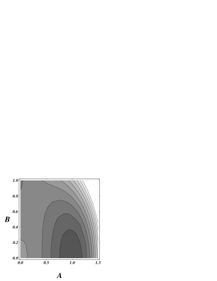
FIG. 3.: Contour plot of the potential surface $V(A,B)$ (22) for the bulk nematic in the physical region $A>0$, $B>0$. The uniaxial amplitude is $A$ and $B$ is the biaxial amplitude. Darker shades indicate lower regions on the potential surface. The isotropic maximum at $(A,B)=(0,0)$ corresponds to a monopole core, the saddle at $(A,B)=(1/4,3/4)$ to a string core, and the minimum at $(A,B)=(1,0)$ to the bulk uniaxial state.

REFERENCES

- [1] G. F. Mazenko, Phys. Rev. B 42, 4487 (1990).
- [2] F. Liu and G. F. Mazenko, Phys. Rev. B 45, 6989 (1992).
- [3] For an excellent review of the field of phase-ordering kinetics see A. J. Bray, Adv. Phys. 43, 357 (1994).
- [4] For a very readable review of the topological theory of defects in ordered media, see N. D. Mermin, Rev. Mod. Phys. 51, 591 (1979).
- [5] R. E. Blundell and A. J. Bray, Phys. Rev. A 46, R6154 (1992).
- [6] H. Toyoki, J. Phys. Soc. Jpn. 63, 4446 (1994).
- [7] I. Chuang, B. Yurke, A. N. Pargellis, and N. Turok, Phys. Rev. E 47, 3343 (1993).
- [8] I. Chuang, R. Durrer, N. Turok, and B. Yurke, Science 251, 1336 (1991).
- [9] For a recent review of the role of defects in both a cosmological and condensed matter context see Formation and Interactions of Topological Defects, edited by A.-C. Davis and R. Brandenberger, NATO ASI Series B: Physics Vol. 349, (Plenum, New York, 1995).
- [10] A. J. Bray, S. Puri, R. E. Blundell, and A. M. Somoza, Phys. Rev. E 47, R2261 (1993).
- [11] A. P. Y. Wong, P. Wiltzius, and B. Yurke, Phys. Rev. Lett. 68, 3583 (1992); A. P. Y. Wong, P. Wiltzius, R. G. Larson, and B. Yurke, Phys. Rev. E 47, 2683 (1993).
- [12] R. C. Desai and A. M. Somoza, cited in reference 20 of [5].
- [13] N. Schopohl and T. J. Sluckin, Phys. Rev. Lett. 59, 2582 (1987).
- [14] F. Liu and G. F. Mazenko, Phys. Rev. B 46, 5963 (1992).
- [15] G. F. Mazenko and R. A. Wickham, Phys. Rev. E 55, 1321 (1997).
- [16] R. A. Wickham, (in preparation).
- [17] A. N. Pargellis, J. Mendez, M. Srinivasarao, and B. Yurke, Phys. Rev. E 53, R25 (1996).
- [18] This can be seen by examining the explicit expression for the charge on a defect, given in [14]. For small distances from the defect core a charge defect has in the model. For a nematic this would represent a charge defect, using the standard definitions [25].
- [19] G. F. Mazenko, Phys. Rev. E 49, 3717 (1994).
- [20] R. A. Wickham and G. F. Mazenko, Phys. Rev. E 55, 2300 (1997).
- [21] A. J. Bray and S. Puri, Phys. Rev. Lett. 67, 2670 (1991); H. Toyoki, Phys. Rev. B 45, 1965 (1992).
- [22] G. Porod, in Small Angle X-Ray Scattering, edited by O. Glatter and L. Kratky (Academic, New York, 1982).
- [23] T. Ohta, D. Jasnow and K. Kawasaki, Phys. Rev. Lett. 49, 1223 (1982).
- [24] A. Poniewierski and T. J. Sluckin, Mol. Phys. 55, 1113 (1985).
- [25] P. G. de Gennes and J. Prost, The Physics of Liquid Crystals 2nd ed. (Clarendon, Oxford, 1993).
- [26] This mapping has been used in equilibrium theories: D. C. Wright and N. D. Mermin, Rev. Mod. Phys. 61, 385 (1989); M. W. Deem, Phys. Rev. E 54, 6441 (1996).
- [27] T. Nagaya, H. Hotta, H. Orihara, and Y. Ishibashi, J. Phys. Soc. Jpn. 61, 3511 (1992); A. N. Pargellis, S. Green, and B. Yurke, Phys. Rev. E, 49, 4250 (1994).
- [28] This special state of affairs is due to a judicial choice of coefficients in the potential (21). However, the scaling properties of the late-time regime are independent of the details of the potential. Thus this particular choice is simply convenient - any potential with the same generic properties is expected to give the same scaling results.
- [29] H. Toyoki and K. Honda, Prog. Theor. Phys. 78, 237 (1987).
- [30] N. Schopohl and T. J. Sluckin, J. Phys. France 49, 1097 (1988).
- [31] G. F. Mazenko and R, A, Wickham, Phys. Rev. E 55, 5113 (1997).
- [32] G. F. Mazenko and R. A. Wickham, submitted to Phys. Rev. E.
- [33] I. S. Gradshteyn and I. M. Ryzhik, Table of Integrals, Series, and Products ed. (Academic, New York, 1994).