Averaged Green function and density of states for electrons in a high magnetic field and random potential

Abstract

We consider a model for $2D$ electrons in a very strong magnetic field (i.e. projected onto a single Landau level) and a random potential $V$. The computation of the averaged Green function for this system reduces to calculating the averaged density of states. We have constructed a computer algebra program which automatically generates a perturbation expansion in $V$ for these quantities. This is equivalent to computing moments of the density of states. When $V$ is a sum of Gaussians from Poisson distributed impurities, each term in the perturbation expansion can be evaluated automatically. We have done so up to $12th$ order. The resulting information can be used to reconstruct the density of states to good precision.

cond-mat/9707153
Theoretical Physics Seminar in Trondheim No. 9 1997 3

[Averaged Green function and density of states]

1 Introduction

The Quantum Hall effects has continued to furnish theoretical physics with challenges and interesting problems for almost twenty years. Is is remarkable that the combination of basic physics (classical electrostatics and magnetism, and non-relativistic quantum mechanics) which has been known and researched upon for so long can lead to so many unexpected and exotic phenomena.

In the work reported on in this paper we have been inspired by the integer Quantum Hall effect[Klitzing] to initiate a somewhat prosaic (but we think nevertheless useful) project — the brute force high order perturbation expansion of impurity averaged quantities in the Quantum Hall system. The problem we consider is a model of non-interacting electrons confined to a two-dimensional layer in a very strong perpendicular magnetic field and a random impurity potential $V$. All information about the physical properties of this model is encoded in its various Green functions. In the absence of electron–electron interactions it suffices to consider the one-particle Green function, e.g. the solution to an equation like

$$-\case{\partial}{\partial t}G({\vec{r}},{\vec{\rho}};t)=HG({\vec{r}},{\vec{\rho}};t),$$

where $H$ is the one-particle Hamiltonian. Thus, $G$ is a random quantity (being a functional of $V$) for which we can only expect to be able to compute various impurity averages like $\overline{\prod_{k=1}^{K}G({\vec{r}}_{k},{\vec{\rho}}_{k};t_{k})}$. In this paper we shall only consider the case of $K=1$. To investigate transport properties one must also consider the case of $K=2$.

Our perturbation expansion consists of expanding $G$ into a series in powers of $V$ (which for our model is equivalent to an expansion in powers of time), and performing the impurity average of each term in this series. The result of the averaging process can be represented by a sum of (Feynman) diagrams. The number of diagrams grows quite rapidly with the perturbative order, to $12$’th order it reaches a few hundred thousand (the exact numbers are listed in Table 1). We have written a computer algebra program which automatically generates all diagrams to a given order.

The use of the generated diagrams is not restricted to the Quantum Hall system. However, the great simplification which occurs for this system (under conditions explained below) is that each diagram reduces to a low-dimensional Gaussian integral (or the integral of a Gaussian multiplied by a polynomial), and thus can be evaluated analytically by computer algebra. The conditions are i) that the system is projected onto a single Landau level (most simply the lowest one), and ii) that all correlators $\overline{V({\vec{r}}_{1})\cdots V({\vec{r}}_{k})}$, can be written as a sum of Gaussians (or Gaussians multiplied by polynomials). The latter restriction is fulfilled if we assume $V$ to arise from a density of Poisson distributed impurities with a Gaussian impurity potential. In the $\delta$-function limit, when the range of the Gaussian goes to zero, this model belongs to a class of systems which was solved exactly for the density of states by Brézin et. al.[Brezin] (a simpler system, which corresponds to the additional limit of taking the impurity density to infinity, was solved earlier by Wegner[Wegner]. These solutions provide useful checks of our results and methodology.

Given the beginning of a perturbation series, even to high orders, it is not obvious how one should extract the correct physical information from it, if its expansion parameter fail to be small. It is not even obvious that computing a few more terms in the perturbation expansion will be helpful. This is a problem which arises quite often, and for which many methods of massaging the perturbation expansions have been devised. Our model provide a non-trivial example of this problem, which can be investigated to rather high order of perturbation theory. We have considered the most common methods of summing infinite subsets of the perturbation series. The results were not encouraging. This is not surprising, in view of the fact that such subsets are usually selected more by their property of being (easily) summable than by their physical importance.

A more fruitful approach to our problem is to utilize the fact that the information contained in the $n$’th perturbative order is equivalent to the $n$’th moment(s) of a spectral function. For the averaged Green function this spectral function is actually the density of states (as function of energy). This is due to the fact that translation invariance forces the relation

$$\overline{G({\vec{x}},{\vec{y}};t)}={\cal P}({\vec{x}},{\vec{y}})\,G(t),$$

where ${\cal P}$ is the projection operator onto the given Landau level.

There are, of course, infinitely many spectral functions which reproduce a given finite set of moments. However, for physical systems the assumptions of a certain degree of smoothness and simple asymptotic behaviour are usually reasonable. Then, the high order behaviour of the moments provide information about the tail of the spectral function, while their totality pins down its overall behaviour. We have applied this procedure with very satisfactory results.

The rest of this paper is organized as follows: In section 2 we give a more detailed description of our model and the method of solution. In section 3 we describe some of the functions which naturally occur in the graphical expansion, the relations between them, and the number of graphs contributing to each perturbative order. This information has been used to check the correctness of our computer algebra programs. In section 4 we present our calculated moments, for the lowest Landau level, and give some physical interpretation of the results. In section 5 we discuss the exact results of Brézin et. al. and Wegner, and compare their density of states with various ways to reconstruct it from our computed moments. In section 6 we discuss the more general case of finite range impurity potential, still in the lowest Landau level. In section 7 we make a more restricted analysis for some higher Landau levels.

2 Model and method of solution

We choose units such that the magnetic length, $\ell_{B}=\sqrt{\hbar/eB}$, becomes unity. I.e., we have $(2\pi)^{-1}$ states per area in each Landau level. We measure energies relative to the (unperturbed) energy of the Landau level we project onto, and choose the energy scale such that the impurity potential becomes

$$W({\vec{r}})=\frac{2}{\varrho-1}\,\exp\left(\frac{-{\vec{r}}^{\,2}}{\varrho-1}\right),$$ (1)

with $\varrho>1$. This is normalized to $\int\d{\vec{r}}\,W({\vec{r}})=2\pi$. The limit $\varrho\to 1^{+}$ corresponds to a delta function potential. We assume a density $f/2\pi$ of Poisson distributed impurities, such that the random potential becomes

$$V({\vec{r}})=\sum_{i}W({\vec{r}}-{\vec{s}}_{i}),$$ (2)

where the impurity positions $\{{\vec{s}}_{i}\}$ are independently and homogeneously distributed. I.e., there is on the average $f$ impurities per state in a single Landau level. Since we neglect couplings to other Landau levels the Hamiltonian is simply equal to $V$, which we shall formally view as a perturbation. Thus, the zero’th order Green function equals the (kernel of the) projection operator onto the $\nu$’th Landau level,

$$G^{(0)}({\vec{r}},{\vec{\rho}};t)={\cal P}_{\nu}({\vec{r}},{\vec{\rho}}).$$

An explicit expression for this projection is

$${\cal P}_{\nu}({\vec{r}},{\vec{\rho}})=\frac{1}{2\pi}\exp\left[-\case{1}{4}({\vec{r}}-{\vec{\rho}})^{2}+\case{\i}{2}(x\eta-\xi y)\right]\,\times\,L_{\nu}\left(\case{1}{2}({\vec{r}}-{\vec{\rho}})^{2}\right),$$ (3)

where $(x,y)$ and $(\xi,\eta)$ are the components of ${\vec{r}}$ and ${\vec{\rho}}$ respectively, and $L_{\nu}$ is the $\nu$’th Laguerre polynomial. For completeness we present a derivation of this well known result in LABEL:app:P. Depending on the choice of gauge, the expression (3) may be multiplied by a gauge factor $\exp\left[\i\Gamma({\vec{r}})-\i\Gamma({\vec{\rho}})\right]$. Since ${\cal P}_{\nu}$ is a projection it has the reproducing property,

$$\int\d{{\vec{\rho}}}\;{\cal P}({\vec{r}}_{1},{\vec{\rho}})\,{\cal P}({\vec{\rho}},{\vec{r}}_{2})={\cal P}({\vec{r}}_{1},{\vec{r}}_{2}).$$ (4)

Since $L_{\nu}(0)=1$, it follows from (3) that ${\cal P}_{\nu}({\vec{r}},{\vec{r}})=(2\pi)^{-1}$, in agreement with the fact that it must equal the number of states per area.

A series expansion for the full $G$ can be generated by repeated time integrations,

$$G({\vec{r}},{\vec{\rho}};t)=\sum_{k=0}^{\infty}\frac{(-t)^{k}}{k!}\left[({\cal P}_{\nu}V)^{k}{\cal P}_{\nu}\right]({\vec{r}},{\vec{\rho}}).$$ (5)

We now average over the impurity positions $\{{\vec{s}}_{i}\}$. To this end we temporarily assume the system to be confined to finite area $2\pi N$ with $S=fN$ impurities, and let $N\to\infty$ afterwards. We find

$$U({\vec{r}}_{1},\ldots,{\vec{r}}_{k})\equiv\overline{V({\vec{r}}_{1})\cdots V({\vec{r}}_{k})}=$$

$$\int\,\left(\prod_{i=1}^{S}\,\frac{\d{\vec{s}}_{i}}{2\pi N}\right)\,\prod_{j=1}^{k}\,\sum_{i_{j}=1}^{S}\,W({\vec{r}}_{1}-{\vec{s}}_{i_{1}})\cdots W({\vec{r}}_{k}-{\vec{s}}_{i_{k}}).$$ (6)

                     

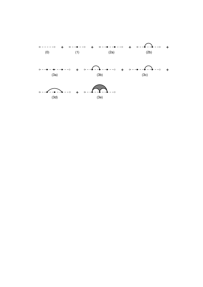
Figure 1: The diagrams for the averaged Green function, up to $3rd$ order in the impurity potential. Open dots represent fixed coordinates, filled dots represent coordinates to be integrated over. A dashed line (with an implicit direction from left to right) represent the projection ${\cal P}_{\nu}$. A full line, or filled regions, represent various correlators of the random potential $V$.

                     

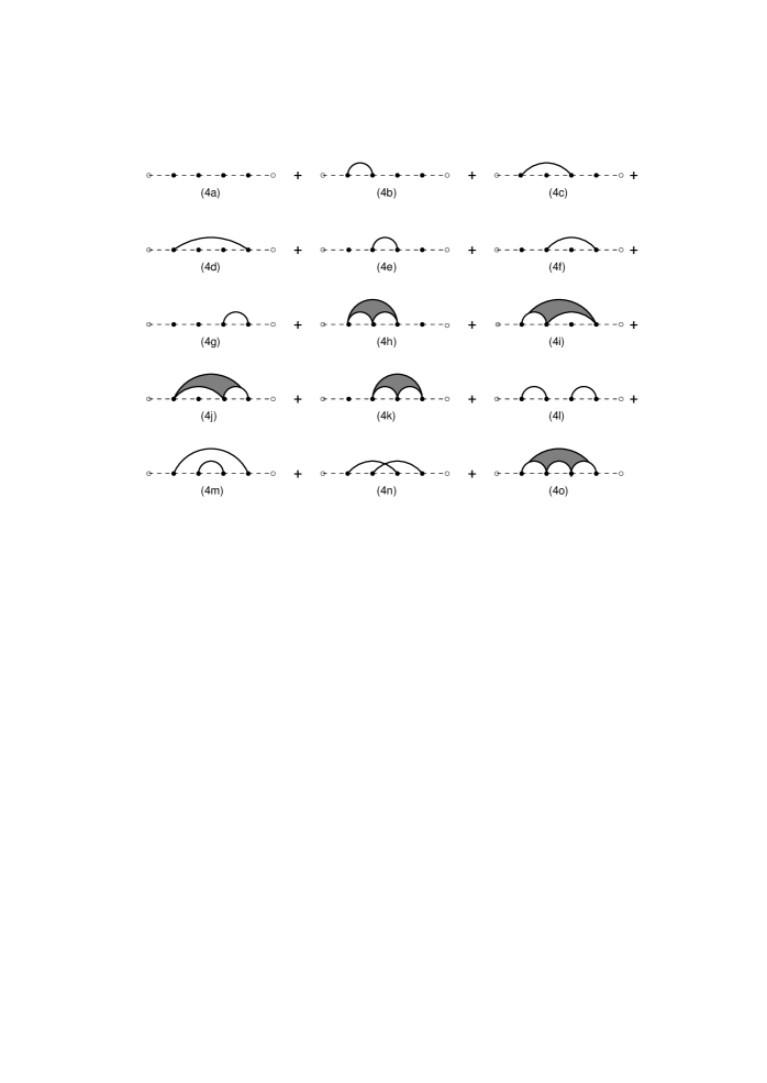
Figure 2: The $4th$ order diagrams for the averaged Green function.

First consider the situation that all the ${\vec{s}}_{i_{j}}$ correspond to different impurities (as is likely the be the case when all the positions ${\vec{r}}_{j}$ are far apart). Then all integrations factorize, each giving a factor $N^{-1}$. Summing over all possible ways to pick $k$ different impurities from a total of $S$, we get the contribution

$$N^{-k}\left(\begin{array}[]{c}S\\ k\end{array}\right)=f(f-\frac{1}{N})\cdots(f-\frac{k-1}{N})\equiv f^{(k)}\to f^{k}\quad\mbox{as $N\to\infty$}$$ (7)

to $U({\vec{r}}_{1},\ldots,{\vec{r}}_{k})$. The other extreme is to assume that all the ${\vec{s}}_{i_{j}}$ correspond to same impurity (as is likely to be the case when the density of impurities is very low, and all the ${\vec{r}}_{i}$’s are close together). Integrating over the impurity position we get a contribution

$$U_{k}({\vec{r}}_{1},\ldots,{\vec{r}}_{k})\equiv\frac{f}{k}\left(\frac{2}{\varrho-1}\right)^{k-1}\exp\left(-\sum_{i,j=1}^{k}\frac{({\vec{r}}_{i}-{\vec{r}}_{j})^{2}}{2k(\varrho-1)}\right)$$ (8)

to $U({\vec{r}}_{1},\ldots,{\vec{r}}_{k})$. The full average must take into account all possible variations between the above two extremes. The complete expression is (as $N\to\infty$)

$$U({\vec{r}}_{1},\ldots,{\vec{r}}_{k})=\sum_{\boldmath\cal Q}U_{a_{1}}({\vec{r}}_{.},\ldots,{\vec{r}}_{.})\cdots U_{a_{j}}({\vec{r}}_{.},\ldots,{\vec{r}}_{.}),$$ (9)

where the sum runs over all partitions $\boldmath\cal Q$ of the set $\{\vec{r}_{1},\ldots,{\vec{r}}_{k}\}$ into $j=1,\ldots,k$ nonempty subsets of sizes $a_{1},\ldots,a_{j}$, and the $U_{a}$’s are symmetric functions of the coordinates in each subset. There are $\sum_{j=1}^{k}{\cal S}^{(j)}_{k}$ terms in the sum, where the ${\cal S}^{(j)}_{k}$’s are the Stirling numbers of the second kind[Abramowitz]. Each term correspond to a Feynman diagram in the perturbation expansion. In our computer algebra program each $k$’th order Feynman diagram is represented by a partition of the set $\{1,\ldots,k\}$. By generating all partitions of this set we obtain all $k$’th order diagrams. They are all topologically distinct, and all occur with combinatorial factor unity.

The 9 diagrams for the $0$’th through $3$’rd order of expansion are shown in figure 1, and the 15 diagrams of $4$’th order are shown in figure 2. Here open dots represent fixed coordinates, and filled dots represent coordinates to be integrated over. A dashed line (with an implicit direction from left to right) represent the projection ${\cal P}_{\nu}$. The symmetric, translation invariant functions $U_{q}({\vec{r}}_{1},\ldots,{\vec{r}}_{q})$ are represented by filled regions connected to $q$ filled dots. For $q=1$ they reduce to isolated filled dots, to each of which there is associated a factor $f$.

According to (8-9), a partition ${\boldmath\cal Q}$ into $j$ nonempty subsets gives a contribution which is proportional to $f^{j}$. This is fully correct only in the limit $N\to\infty$. A finite size correction is obtained by making the replacement $f^{j}\to f^{(j)}$, cf. equation (7).

The evaluation of the individual diagrams amounts to computing integrals like

$$\int\prod_{i=1}^{k}\d{\vec{\rho}}_{i}\;{\cal P}_{\nu}({\vec{r}},{\vec{\rho}}_{1}){\cal P}_{\nu}({\vec{\rho}}_{1},{\vec{\rho}}_{2})\cdots{\cal P}_{\nu}({\vec{\rho}}_{k},{\vec{\rho}})\;U_{a_{1}}({\vec{\rho}}_{.},\ldots,{\vec{\rho}}_{.})\cdots U_{a_{j}}({\vec{\rho}}_{.},\ldots,{\vec{\rho}}_{.})$$

For the lowest Landau level, $\nu=0$, this is just a sum of Gaussian integrals. In the higher levels it becomes a sum of Gaussians multiplied by polynomials.

Since the averaging process restores translation invariance, each diagram must be a translation invariant (with respect to the magnetic translation group) expression constructed only out of states in the $\nu$’th Landau level. This forces it to be proportional to ${\cal P}_{\nu}({\vec{r}},{\vec{\rho}})$. To show this more explicitly, we start with the most general expansion of an averaged diagram,

$$\overline{G_{\boldmath{\cal Q}}({\vec{r}},{\vec{\rho}})}=\int\d{p}\,\d{q}\;C(p,q)\,\psi_{p}({\vec{r}})\,\psi_{q}({\vec{\rho}})^{*},$$

where $\{\psi_{p}\}$ form an orthonormal basis for the $\nu$’th Landau level.

In the Landau gauge, $A^{y}=0$, we may choose this basis such that the magnetic translation group acts as

$$t(a\hat{x}):\psi_{k}\rightarrow\mbox{e}^{ika^{\prime}}\,\psi_{k},\qquad t(b\hat{y}):\psi_{k}\rightarrow\psi_{k+b^{\prime}},$$

where $a^{\prime}$ is proportional to $a$, and $b^{\prime}$ is proportional to $b$. The requirement that

$$\overline{\left[t(b{\hat{y}})G_{\boldmath{\cal Q}}\right]({\vec{r}},{\vec{\rho}})}=\overline{G_{\boldmath{\cal Q}}({\vec{r}},{\vec{\rho}})}$$

implies that $C(p,q)=C(p-q)$, and the requirement that

$$\overline{\left[t(a{\hat{x}})G_{\boldmath{\cal Q}}\right]({\vec{r}},{\vec{\rho}})}=\overline{G_{\boldmath{\cal Q}}({\vec{r}},{\vec{\rho}})}$$

implies that $C(p-q)=C_{0}\,\delta(p-q)$, with $C_{0}$ a constant. Thus, $\overline{G_{\boldmath{\cal Q}}({\vec{r}},{\vec{\rho}})}\propto{\cal P}_{\nu}({\vec{r}},{\vec{\rho}})$. A graphical representation of this relation is illustrated in figure 3 (except that the split-off “vacuum diagram” should not be counted with its usual combinatorial factor). As a control of our computer algebra program, we have verified this relation explicitly for a large number of cases. Using it reduces the evaluation of $k$’th order diagrams to calculating determinants of $k\times k$ matrices (when employing complex coordinates in the lowest Landau level).

                     

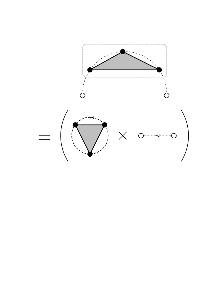
Figure 3: Due to translation invariance, every diagram contributing to the averaged Green function becomes proportional to the projection onto the given Landau level.

Comparing the expansion

$$\overline{G({\vec{r}},{\vec{\rho}};t)}={\cal P}_{\nu}({\vec{r}},{\vec{\rho}})\,\sum_{k=0}^{\infty}\,\frac{(-t)^{k}}{k!}\,G_{k}\equiv{\cal P}_{\nu}({\vec{r}},{\vec{\rho}})\,G(t)$$

with the general expansion in energy eigenfunctions

$$G({\vec{r}},{\vec{\rho}};t)=\sum_{\alpha}\psi_{\alpha}({\vec{r}})\,\psi_{\alpha}^{*}(\vec{\rho})\,\exp\left(-tE_{\alpha}\right),$$

we obtain after setting $\vec{\rho}=\vec{r}$ and integrating

$$N\,G(t)=\overline{\sum_{\alpha}\,\exp\left(-tE_{\alpha}\right)}\equiv N\,\int\d{E}\,D(E)\,\exp\left(-tE\right),$$ (10)

where $D(E)$ is the averaged density of states (normalized to $\int\d{E}D(E)=1$. I.e., $G(t)$ is simply the Laplace transform of $D(E)$, and the information obtained from the $k$’th perturbative order is exactly the $k$’th moment of the averaged density of states,

$$G_{k}=\int\d{E}D(E)\,E^{k}.$$ (11)

3 Counting and resumming graphs

We define

$${\tilde{G}}(u)\equiv-\int_{0}^{\infty}\d{t}\;\mbox{e}^{t/u}\,G(t)=\int\d{E}\;D(E)\,\frac{u}{1-Eu}=\sum_{k=0}^{\infty}G_{k}\,u^{k+1},$$ (12)

where the series should be interpreted in an asymptotic sense. The integral converges for $u<0$, and ${\tilde{G}}(u)$ can be extended by analytic continuation. As noted, the graphical expansion illustrated by figures 1–2 amounts to expanding ${\tilde{G}}$ into a formal power series in $u$. There are various ways to resum graphical expansions of this type. The simplest and most useful one is to sum up sequences of ${\cal P}_{\nu}$’s connected by isolated dots (i.e., factors of $U_{1}$). This amounts to making the replacement ${\cal P}_{\nu}\to{\cal P}_{\nu}\,\frac{1}{1-fu}$, and summing over graphs containing no isolated dots. The latter sum defines a function ${\hat{G}}(u)$, related to ${\tilde{G}}$ by

$${\tilde{G}}(u)={\hat{G}}(\frac{u}{1-fu}).$$ (13)

The $k$’th order graphs for ${\hat{G}}(u)\sim\sum_{k=0}^{\infty}{\hat{G}}_{k}\,u^{k+1}$ are in 1-1 correspondence with the partitions of the set $\{1,\ldots,k\}$ into subsets of sizes $a_{j}\geq 2$. The number of such partitions is significantly smaller than the total number. For instance, inspection of figures 1–2 reveal that only the graphs $(0)$, $(1)$, $(2b)$, $(3e)$, and $(4\ell)$-$(4o)$ contribute to ${\hat{G}}$ up to the $4$’th order. The total numbers of graphs which contribute to ${\tilde{G}}(u)$ ($G_{k}$) and ${\hat{G}}(u)$ (${\hat{G}}_{k}$) are listed in tab:counts.

Table 1: The number of graphs contributing to various functions. $G_{k}$: The total number of graphs contributing to the Green function. ${\hat{G}}_{k}$: The number of graphs not containing isolated dots. ${\hat{\Sigma}}_{k}$: The number of 1-particle irreducible graphs not containing isolated dots. $S_{k}$: The number of skeleton graphs. $C_{k}$: The number of irreducible terms in the answer.

$k$	$G_{k}$	${\hat{G}}_{k}$	$\hat{\Sigma}_{k}$	$S_{k}$	$C_{k}$
1	1	0	0	1	1
2	2	1	1	1	1
3	5	1	1	1	1
4	15	4	3	2	2
5	52	11	9	6	2
6	203	41	33	21	7
7	877	162	135	85	10
8	4 140	715	609	385	36
9	21 147	3 425	2 985	1 907	85
10	115 975	17 722	15 747	10 205	319
11	678 570	98 253	88 761	58 455	1 113
12	4 213 597	580 317	531 561	355 884	5 088
13	27 644 437	3 633 280	3 366 567	2 290 536
14	190 899 322	24 011 157	22 462 017	15 518 391
15	1 382 958 545	166 888 165	157 363 329	110 283 179
16	10 480 142 147	1 216 070 389	1 154 257 683	819 675 482

Another standard resummation is to define $\Sigma(u)$ through the relation

$${\tilde{G}}(u)=\frac{u}{1-\Sigma(u)},$$ (14)

where only 1-particle irreducible graphs contribute to $\Sigma$. We may combine this with the resummation of isolated dots above, to obtain

$$\Sigma(u)=fu+(1-fu){\hat{\Sigma}}(\frac{u}{1-fu}).$$ (15)

Here ${\hat{\Sigma}}$ is the sum of all 1-particle irreducible graphs which do not contain isolated dots. The numbers of such graphs are also listed in tab:counts. As can be seen, there is some reduction in the number of graphs to be calculated, but not a very significant one. Of the graphs in figures 1–2, the only additional saving is the elimination of graph $(4\ell)$.

A further reduction in the number of contributing graphs is obtained by first summing the up the skeleton diagrams $S(u)$. This is the set of graphs such that their corresponding “vacuum diagrams” (cf. figure 3) are 1-particle irreducible. This function is related to $\Sigma$ by

$$\Sigma(u)=\left[1-\Sigma(u)\right]\,S(\frac{u}{1-\Sigma(u)}).$$ (16)

(The function ${\hat{S}}(u)=S(u)-fu$ is related to ${\hat{\Sigma}}(u)$ in the same way.) The numbers of graphs contributing to $S$ are also listed in tab:counts. Expanding $S$ to second order in its argument, and solving the resulting 2nd degree algebraic equation for $\Sigma$ (or, equivalently, $\tilde{G}$), constitutes to the so-called self consistent Born approximation (SCBA). Of the graphs in figures 1–2, the only additional saving when restricting to skeleton diagrams is the elimination of graph $(4m)$.

One way to employ the resummation methods above is to generate a smaller set of diagrams (e.g., for ${\hat{G}}(u)$, ${\hat{\Sigma}}(u)$, or $S(u)$) to a given order, and then find the full perturbation expansion to the same order by use of the algebraic relations above. However, the benefits of going beyond ${\hat{G}}(u)$ are marginal, since the reduction in number of graphs is rather small while more computer time is needed to classify graphs. We have in our computation evaluated all graphs contributing to ${\hat{G}}(u)$. As a check on the computer algebra we have in addition summed the subsets of these graphs contributing to ${\hat{\Sigma}}(u)$ and $S(u)$, and verified that they reproduce the same end result for $G(u)$. The simplest check of the program is to verify that it actually generates the number of graphs listed in tab:counts, since these numbers are computed in an entirely independent way (starting from the Stirling numbers).

Another way to use the resummation methods above is to combine a finite perturbation expansion from $\hat{\Sigma}(u)$ or $S(u)$ with the exact algebraic equations, thereby generating some approximate, but infinite, series for $G(u)$. Considering the numbers in tab:counts, we note that the resummation of isolated dots captures a large percentage of the total number of graphs. However, the physical effect of this resummation is rather uninteresting—it merely corresponds to an overall shift in the energies. Of the remaining graphs we note that the majority of them are complicated ones (i.e., skeleton graphs) which cannot be generated by resumming lower order terms. Thus, the resummations above underestimate the $k$’th perturbative order by increasingly large amounts as $k$ increases. In the absence of any physical reasons for selecting a particular class of diagrams, we believe it is much more sensible to extrapolate the perturbation series in a statistical sense, by considering how the total number of graphs, and their average value, varies with the perturbative order $k$.

4 Calculated moments

We have calculated the perturbation series up to the $12$’th perturbative order, for general values of impurity density $f$ and potential range $\varrho$. Each graph contributes a rational function in $\varrho$, multiplied by some power of $f$. The general answer rapidly becomes too complicated to present here. We present the result in terms of the moments $G_{k}$ of the density of states. The general expressions for the first five moments are listed in tab:xi. The full result for the case of $\delta$-function impurities, $\varrho=1$, is listed in tab:xi0. We list results for some additional values of $\varrho$ (in floating point form) in LABEL:app:CumTabs.

Table 2: The first five energy moments for general $\varrho$, in the lowest Landau level.

$k$	$G_{k}$
1	$f$
2	${\frac{1}{\varrho}}f+{f}^{2}$
3	${\frac{4}{3\,{\varrho}^{2}+1}}f+{\frac{3}{\varrho}}{f}^{2}+{f}^{3}$
4	${\frac{2}{\varrho\,\left({\varrho}^{2}+1\right)}}f+{\frac{25\,{\varrho}^{4}+25\,{\varrho}^{2}+2}{{\varrho}^{2}\left({\varrho}^{2}+1\right)\left(3\,{\varrho}^{2}+1\right)}}{f}^{2}+{\frac{6}{\varrho}}{f}^{3}+{f}^{4}$
5	${\frac{16}{5\,{\varrho}^{4}+10\,{\varrho}^{2}+1}}f+{\frac{210\,{\varrho}^{4}+420\,{\varrho}^{2}+170}{\varrho\,\left(3\,{\varrho}^{2}+1\right)\left(3\,{\varrho}^{2}+5\right)\left({\varrho}^{2}+1\right)}}{f}^{2}+{\frac{85\,{\varrho}^{4}+85\,{\varrho}^{2}+10}{{\varrho}^{2}\left({\varrho}^{2}+1\right)\left(3\,{\varrho}^{2}+1\right)}}{f}^{3}+{\frac{10}{\varrho}}{f}^{4}+{f}^{5}$
⋮
$k$	$\frac{2^{k}}{(\varrho+1)^{k}-(\varrho-1)^{k}}f+\cdots+{k\choose 3}\frac{(9k-11)(\varrho^{4}+\varrho^{2})+(2k-6)}{4\varrho^{2}(\varrho^{2}+1)(3\varrho^{2}+1)}f^{k-2}+\frac{k(k-1)}{2\varrho}f^{k-1}+f^{k}$

Table 3: The twelve first energy moments for $\delta$-function impurities ($\varrho=1$).

$k$	$G_{k}$
1	$f$
2	$f+{f}^{2}$
3	$f+3\,{f}^{2}+{f}^{3}$
4	$f+{\frac{13}{2}}{f}^{2}+6\,{f}^{3}+{f}^{4}$
5	$f+{\frac{25}{2}}{f}^{2}+{\frac{45}{2}}{f}^{3}+10\,{f}^{4}+{f}^{5}$
6	$f+{\frac{137}{6}}{f}^{2}+{\frac{277}{4}}{f}^{3}+{\frac{115}{2}}{f}^{4}+15\,{f}^{5}+{f}^{6}$
7	$f+{\frac{245}{6}}{f}^{2}+{\frac{2317}{12}}{f}^{3}+{\frac{1029}{4}}{f}^{4}+{\frac{245}{2}}{f}^{5}+21\,{f}^{6}+{f}^{7}$
8	$f+{\frac{871}{12}}{f}^{2}+{\frac{3067}{6}}{f}^{3}+{\frac{24131}{24}}{f}^{4}+749{f}^{5}+231{f}^{6}+28{f}^{7}+{f}^{8}$
9	$f+{\frac{517}{4}}{f}^{2}+{\frac{47443}{36}}{f}^{3}+{\frac{29091}{8}}{f}^{4}+{\frac{31121}{8}}{f}^{5}+1848{f}^{6}+399{f}^{7}+36{f}^{8}+{f}^{9}$
10	$f+\frac{4629}{20}f^{2}+\frac{241715}{72}f^{3}+\frac{452455}{36}f^{4}+\frac{292901}{16}f^{5}+\frac{98261}{8}f^{6}+\frac{8085}{2}f^{7}+645f^{8}$
	$+45f^{9}+f^{10}$
11	$f+\frac{8349}{20}f^{2}+\frac{3068197}{360}f^{3}+\frac{3047209}{72}f^{4}+\frac{11665093}{144}f^{5}+\frac{1163173}{16}f^{6}+\frac{267377}{8}f^{7}$
	$+\frac{16137}{2}f^{8}+990f^{9}+55f^{10}+f^{11}$
12	$f+\frac{45517}{60}f^{2}+\frac{5201203}{240}f^{3}+\frac{303556067}{2160}f^{4}+\frac{16554385}{48}f^{5}+\frac{114943133}{288}f^{6}$
	$+\frac{1940433}{8}f^{7}+\frac{649231}{8}f^{8}+14982f^{9}+\frac{2915}{2}f^{10}+66f^{11}+f^{12}$

It is an amusing exercise to search for general patterns in tab:xi and tab:xi0. The coefficients of the highest powers of $f$ are straightforward to find, since the series for ${\hat{G}}(u)$ up to the $2j$’th perturbative order determines all the terms proportional to $f^{k}$, $f^{k-1}$, …, $f^{k-j}$ in the $k$’th perturbative order. The lowest powers of $f$ are of more physical interest. Consider first the case of $\delta$-function impurities. The general pattern of the $f^{2}$-terms looks a bit complicated, but it is easy to verify that it fits the formula

$$G_{k}=f+f^{2}\,\sum_{p=1}^{\lfloor k/2\rfloor}\,\frac{1}{p}\left(\begin{array}[]{c}k\\ 2p\end{array}\right)+\Or(f^{3}).$$ (17)

These moments are reproduced to order $f^{2}$ by the density of states

$$D(E)=(1-f)\,\delta(E)+\case{1}{2}\,f^{2}\,\theta(E)\,\theta(2-E)\,|E-1|^{f-1}.$$ (18)

The physics behind this expression is as follows:

1. Consider $S=fN<N$ arbitrary placed impurities in a single Landau level, for which the Hilbert space of wave functions is $N$-dimensional. The condition that a wave function vanishes on all impurities imposes $S$ constraints, for which the solution space is at least $(N-S)$-dimensional. These solutions will have exactly zero energy, which is also the lowest possible energy. Hence, there must for all $f<1$ be a $\delta$-function contribution to the density of states, of strength $(1-f)$.

2. At very low $f$ the impurities are very far apart. Each of them will bind one state of energy $E=1$. Hence, they will contribute a term $f\,\delta(E-1)$ to the density of states. This is sufficient to reproduce all moments to order $f$. To order $f^{2}$ we must consider the mixing between states at different impurities (to this order only mixing between two impurities). The energies for two impurities at distance $r$ are $E_{\pm}=1\pm\mbox{e}^{-r^{2}/4}$. Integrating over the distribution of relative distances we get a contribution to the density of states,

   $$\Delta D(E)\propto\int\d{\vec{r}}\;\left[\delta(E-1-\mbox{e}^{-r^{2}/4})+\delta(E-1+\mbox{e}^{-r^{2}/4})\right]$$

   $$\propto\int_{0}^{1}\frac{\d{x}}{x}\,\left[\delta(E-1-x)+\delta(E-1+x)\right]$$

   $$\propto\;\theta(E)\,\theta(2-E)\,|E-1|^{-1}.$$

   This distribution is not normalizable, but has finite moments $\langle(E-1)^{k}\rangle$. The lack of normalization is due to the fact that additional impurities must be taken into account at very large separations $r$ (of order $f^{-1/2}$). A simple way to model this is by introducing a distribution $dp(r)=\mbox{e}^{-kfr^{2}}kfdr^{2}$ for the relative pair distance (the total density of pairs being $\frac{1}{2}f$). The requirement that all moments be reproduced to order $f^{2}$ fixes $k=\frac{1}{4}$. This in turn leads to (18).

3. If one repeat the previous argument with the finite size correction, $f^{2}\to f^{(2)}=f(f-N^{-1})$, one is lead to the conclusion that the exponent in (18) should also undergo a finite size correction,

   $${|E-1|}^{f-1}\to{|E-1|}^{f-1-1/N}.$$

It is also easy to understand the physical origin of the low-$f$ behaviour of the general moments,

$$G_{k}=\frac{2^{k}}{(\varrho+1)^{k}-(\varrho-1)^{k}}\,f+\Or(f^{2}).$$ (19)

This is related to the behaviour of electrons near the single impurity potential (1). With the impurity at the origin we find eigenstates (in the symmetric gauge, and cylinder coordinates)

$$\psi_{\ell}({\vec{r}})=(2\pi\,2^{\ell}\,\ell!)^{-1/2}\;r^{\ell}\,\e^{-\i\ell\varphi}\,\e^{-r^{2}/4},$$

and corresponding energies (cf. Appendix A)

$$E_{\ell}=\left(\frac{2}{\varrho+1}\right)\left(\frac{\varrho-1}{\varrho+1}\right)^{\ell},\qquad\ell=0,1,2,\ldots.$$ (20)

With a small fraction $f$ of such impurities the contribution to the density of states becomes

$$D(E)=f\,\sum_{\ell}\delta(E-E_{\ell}).$$ (21)

The sum must be cut off when the extension $r_{\ell}$ of the wave function becomes of order $f^{-1/2}$, i.e. for $\ell$ of order $f^{-1}$. This is important for obtaining a normalized $D$, but can be ignored when calculating its moments. Thus we get to order $f$

$$G_{k}=f\;\sum_{\ell=0}^{\infty}\,E_{\ell}^{k}=f\;\left(\frac{2}{\varrho+1}\right)^{k}\,\left[1-\left(\frac{\varrho-1}{\varrho+1}\right)^{k}\right]^{-1}.$$

4.1 The cumulant expansion

The information in tab:xi and tab:xi0 can be compressed somewhat by rewriting it in terms of cumulants. The moments $\langle E^{k}\rangle$ are related to the Laplace transform of the density of states,

$$G(t)\equiv\int_{0}^{\infty}\d{E}\,D(E)\,\e^{-tE}=\sum_{k=0}^{\infty}\frac{(-t)^{k}}{k!}\,G_{k}.$$ (22)

By rewriting

$$G(t)=\exp\left(\chi(t)\right)=\exp\left(\sum_{k=1}^{\infty}t^{k}\,\chi_{k}\right)$$ (23)

we obtain the cumulant expansion. No information is lost when going between the set of cumulants $\{\chi_{k}|k=1,\ldots,m\}$ and the set of moments $\{G_{k}|k=1,\ldots,m\}$.

Table 4: The first five cumulants for general $\varrho$, in the lowest Landau level.

$k$	$(-1)^{k}\,k!\,\chi_{k}$
1	$f$
2	${\frac{1}{\varrho}}f$
3	${\frac{4}{3\,{\varrho}^{2}+1}}f$
4	${\frac{2}{\varrho\,\left({\varrho}^{2}+1\right)}}f-{\frac{1}{\left({\varrho}^{2}+1\right){\varrho}^{2}}}{f}^{2}$
5	${\frac{16}{5\,{\varrho}^{4}+10\,{\varrho}^{2}+1}}f-{\frac{80}{\left(3\,{\varrho}^{2}+5\right)\varrho\,\left(3\,{\varrho}^{2}+1\right)}}{f}^{2}$
$\vdots$
$k$	$\frac{2^{k}}{(\varrho+1)^{k}-(\varrho-1)^{k}}f+\cdots$

Table 5: The 12 first cumulants for $\delta$-function impurities, in the lowest Landau level.

$k$	$(-1)^{k}\,k!\,\chi_{k}$
1	$f$
2	$f$
3	$f$
4	$f-{\frac{1}{2}}{f}^{2}$
5	$f-{\frac{5}{2}}{f}^{2}$
6	$f-{\frac{49}{6}}{f}^{2}+{\frac{7}{4}}{f}^{3}$
7	$f-{\frac{133}{6}}{f}^{2}+{\frac{77}{4}}{f}^{3}$
8	$f-{\frac{653}{12}}{f}^{2}+{\frac{757}{6}}{f}^{3}-{\frac{109}{8}}{f}^{4}$
9	$f-{\frac{503}{4}}{f}^{2}+{\frac{11603}{18}}{f}^{3}-{\frac{2085}{8}}{f}^{4}$
10	$f-\frac{5591}{20}f^{2}+\frac{204725}{72}f^{3}-\frac{17065}{6}f^{4}+\frac{2971}{16}f^{5}$
11	$f-\frac{12111}{20}f^{2}+\frac{820787}{72}f^{3}-\frac{841489}{36}f^{4}+\frac{87197}{16}f^{5}$
12	$f-\frac{77303}{60}f^{2}+\frac{10270399}{240}f^{3}-\frac{69677951}{432}f^{4}+\frac{87197}{16}f^{5}-\frac{124513}{32}f^{6}$

We show the five first cumulants for general values of $f$ and $\varrho$ in tab:chi, and the twelve first cumulants for $\delta$-function potentials ($\varrho=1$) in tab:chi0. Note that a factor $(-1)^{k}/k!$ has been split off in both tables. The cumulant expansion may also be viewed as yet another way of resumming a perturbation expansion. We return to this below.

5 Comparison with the exact results of Brézin et. al. and Wegner

For the case of $\delta$-function impurities, $\varrho=1$, exact formulas for the density of states have been found by Brézin et. al.[Brezin], and by Wegner[Wegner]. The result by Wegner correspond to taking the additional limit of $f\to\infty$. Their expressions for the density of states are highly non-trivial, and they provide very useful checks on our results and methodology.

5.1 The result of Brézin et. al.

                     

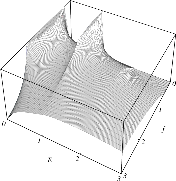
Figure 4: A $3D$-plot of the density of states found by Brézin et. al., as function of energy $E$ and impurity density $f$. In addition to the plotted density there is a contribution $(1-f)\,\delta(E)$ when $f<1$.

The results found in reference [Brezin] specializes for our model (with $\varrho=1$) to the integral

$$D_{{\mathrm{B}}}(E)=\frac{1}{\pi}\,{\mathrm{I}m}\frac{\partial}{\partial E}\ln\int_{0}^{\infty}\d{t}\,\exp[\,\i Et-f\,I(t)\,]\,,\qquad{\rm where}$$

$$I(t)=\int_{0}^{t}\frac{\d{\beta}}{\beta}\left(1-\e^{-\i\beta}\right)=\i t+{\tsty\frac{1}{4}}\,t^{2}-{\tsty\frac{\i}{18}}\,t^{4}-\cdots.$$ (24)

It is a rather challenging task to evaluate this expression numerically. As was pointed out in [Brezin], $D_{{\mathrm{B}}}(E)$ has a lot of interesting structure, in particular for low density of impurities $f$:

1. For $f<1$ there is a $\delta$-function contribution to $D_{{\mathrm{B}}}(E)$,

   $$D_{{\mathrm{B}}}(E)=(1-f)\,\delta(E)+\cdots.$$ (25)

   As explained before (cf. the discussion around equation (18)), this is due to the fact that we may arrange for a fraction $1-f$ of all wavefunctions to vanish on all impurities. This phenomenon was already pointed out by Ando[Ando].

2. As $E\to 0^{+}$ one finds the behaviour

   $$D_{{\mathrm{B}}}(E)\sim\left\{\begin{array}[]{ll}E^{-f}&0<f<1,\\ E^{-1}/\log^{2}(E)&f=1,\\ E^{f-2}&1<f.\end{array}\right.$$ (26)

   The increasingly singular behaviour as $f$ increases from $0$ to $1$ is due to zero-energy states moving out into the low $E$ region. As for the large $f$-dependence, a crude qualitative understanding is obtained by considering an arbitrary placed, maximally localized state,

   $$|\psi({\vec{r}})|^{2}={\cal N}\,\e^{-({\vec{r}}-{\vec{r}}_{0})^{2}/2}.$$

   The probability $\mbox{Prob}(E<E_{0})$ that this state has an energy less that $E_{0}$ is equal to the probability that the distance $r$ from ${\vec{r}}_{0}$ to its nearest impurity satisfies ${\cal N}\,\exp(-r^{2}/2)<E_{0}$. Now,

   $$\mbox{Prob}\left(\exp(-r^{2}/2)<E_{0}/2\pi{\cal N}\right)=\left({E_{0}}/2\pi{\cal N}\right)^{f},$$

   which predicts $D(E)\sim E^{f-1}$. This is an underestimate (because our assumption that the state was maximally localized, and arbitrary placed, cannot be expected to hold), but the dependence on $f$ turns out to be correct.

3. As $E\to 1$ one finds a diverging density of states

   $$D_{{\mathrm{B}}}(E)\sim|E-1|^{f-1},\quad\mbox{for $0<f<1$,}$$ (27)

   and this singularity continues as a cusp singularity for $1<f<2$. As discussed before (cf. equation (18)), this singularity originates in states localized on top of single impurities. The interaction with nearby impurities leads to a level broadening around $E=1$.

4. As $E\to 2$ there is a cusp singularity,

   $$\frac{d}{dE}D_{{\mathrm{B}}}(E)\sim|E-2|^{f-1},\quad\mbox{for $0<f<1$.}$$ (28)

   This singularity is due to the fact that a state must interact with at least three impurities to have an energy $E>2$, while two impurities are sufficient for $E<2$. By a similar reasoning one can also understand why there are (increasingly weak) singularities in $D_{{\mathrm{B}}}(E)$ at $E=3,4,\ldots$.

5. $D_{{\mathrm{B}}}(E)$ is a fairly smooth function for $f>2$.

                     

Figure 5: The density of state for a) $f=0.2$, b) $f=0.5$, and c) $f=0.8$. Due to a $\delta$-function contribution at $E=0$ the curves are normalized to $f$ instead of 1.

Plots for the integrated density of states, $\int_{0}^{E}\d{E}^{\prime}D_{{\mathrm{B}}}(E^{\prime})$, where given in [Brezin] and [ItzyksonDrouffe]. The plots of $D_{{\mathrm{B}}}(E)$ itself look more interesting; we give examples in figures 4-5. We shall return to the a reconstruction of $D_{{\mathrm{B}}}(E)$ from our calculated moments, but first consider the limiting case of $f\to\infty$.

5.2 The limit of high impurity density, and the result of Wegner

Consider now equation (24) for very large $f$. The main contribution to the integral will come from small $t$, hence we may approximate

$$I(t)\approx it+\case 14t^{2}.$$ (29)

This leads to the expression

$$\sqrt{f}\,D_{{\mathrm{B}}}(E)\approx D_{{\mathrm{W}}}(\epsilon)\equiv\frac{1}{\pi}\,{\mathrm{I}m}\frac{\partial}{\partial\epsilon}\ln\left(1+\mbox{erf}(\i\epsilon)\right)$$

$$=\frac{2}{\pi^{3/2}}\,\frac{\exp(\epsilon^{2})}{1-\mbox{erf}^{\,2}(\i\epsilon)}=\frac{2}{\pi^{3/2}}\,\frac{\exp(\epsilon^{2})}{1+\mbox{irf}^{\,2}(\epsilon)},$$ (30)

where $\epsilon=(E-f)/\sqrt{f}$, and $\mbox{irf}(\epsilon)\equiv-\i\,\mbox{erf}(\i\epsilon)$ is a real function of a real argument. This is equivalent to the result by Wegner[Wegner].

The Fourier transform of $D_{{\mathrm{W}}}(\epsilon)$ has the series expansion

$${\tilde{D}}_{{\mathrm{W}}}(\omega)=\int_{-\infty}^{\infty}\d{\epsilon}\,\e^{-\i\,\omega\,\epsilon}D_{{\mathrm{W}}}(\epsilon)$$

$$=1-{\tsty\frac{1}{2!}}\,\langle\epsilon^{2}\rangle\,\omega^{2}+{\tsty\frac{1}{4!}}\,\langle\epsilon^{4}\rangle\,\omega^{4}-{\tsty\frac{1}{6!}}\,\langle\epsilon^{6}\rangle\,\omega^{6}+{\tsty\frac{1}{8!}}\,\langle\epsilon^{8}\rangle\,\omega^{8}-\cdots,$$ (31)

with $\langle\epsilon^{n}\rangle=\int_{-\infty}^{\infty}\d{\epsilon}\,D_{{\mathrm{W}}}(\epsilon)\,\epsilon^{n}$. One may verify (numerically) that

$$\fl\langle\epsilon^{2}\rangle=1,\ \langle\epsilon^{4}\rangle=\case 52,\ \langle\epsilon^{6}\rangle={\tsty\frac{37}{4}},\ \langle\epsilon^{8}\rangle={\tsty\frac{353}{8}},\ \langle\epsilon^{10}\rangle={\tsty\frac{4081}{16}},\ \langle\epsilon^{12}\rangle={\tsty\frac{55205}{32}}.$$ (32)

All odd moments vanish because $D_{{\mathrm{W}}}(\epsilon)$ is an even function of $\epsilon$.

Now turn to the problem of determining $D(E)$ from e.g. the cumulants in table 4. Formally this may be done by inverting the Laplace transform (22-23). With $t=\i u$ this becomes

$$D(E)={\frac{1}{2\pi}}\int_{-\infty}^{\infty}\d{u}\,\e^{i(E-f)u}\,\exp\sum_{k=2}^{\infty}(\i u)^{k}\chi_{k}.$$ (33)

To investigate the large-$f$ limit we introduce $\epsilon=(E-f)/\sqrt{f}$, $\omega=u\sqrt{f}$, and keep only terms which remain when $f\to\infty$. Thus, in this limit,

$$\sqrt{f}\,D(E)\approx\frac{1}{2\pi}\int_{-\infty}^{\infty}\d{\omega}\,\e^{\i\epsilon\omega}\,{\tilde{D}}(\omega),$$ (34)

where we find from table 4

$$\fl{\tilde{D}}(\omega)=\exp\left(-\case 12\,\omega^{2}-{\tsty\frac{1}{2\cdot 4!}}\,\omega^{4}-{\tsty\frac{7}{4\cdot 6!}}\,\omega^{6}-{\tsty\frac{109}{8\cdot 8!}}\,\omega^{8}-{\tsty\frac{2971}{16\cdot 10!}}\,\omega^{10}-{\tsty\frac{124513}{32\cdot 12!}}\,\omega^{12}-\cdots\right).$$ (35)

One may verify that $D_{{\mathrm{W}}}(\omega)=D(\omega)$ to the order in $\omega$ we have computed.

5.3 From cumulant expansion to density of states

We now construct approximants $D_{n}(\epsilon)$ to $D(\epsilon)$, using equation (33) with the cumulants $\chi_{2},\ldots,\chi_{n}$ included in the sum. The result is surprising and instructive. To investigate convergence we evaluate the densities at $\epsilon=0$ for increasing $n$. We find

$$D_{n}(0)=(0.3788,0.3744,03721,0.3710,0.3703)\mbox{ for $n=(4,6,8,10,12)$.}$$

This sequence converges nicely with $n$ (see figure 6), fitting the formula

$$D_{n}(0)\approx 0.3675+0.02456\,n^{-1}+0.09745\,n^{-2}+\cdots.$$

However, when extrapolated to $n=\infty$ we obtain $D_{\infty}(0)\approx 0.3675$, which is about $2.3$ percent higher than the exact result,

$$D_{{\mathrm{W}}}(0)=2/\pi^{3/2}=0.35917\ldots.$$

                     

Figure 6: The approximants $D_{n}(0)$ as function of $n^{-1}$, together with a fitting function. It is clear that the approximants converges to a value which is different from the (indicated) exact result, $D_{{\mathrm{W}}}(0)=0.35917\ldots$

                     

Figure 7: A comparison of the approximants $D_{10}(\epsilon)$ and $D_{12}(\epsilon)$ (dashed lines) with the exact result $D_{{\mathrm{W}}}(\epsilon)$ (fully drawn line). Since all curves are symmetric with respect to $\epsilon\to-\epsilon$ only positive $\epsilon$ is plotted. $D_{10}$ and $D_{12}$ are almost indistinguishable, indicating good convergence. However, the approximants have converged to a result which is different from the exact one.

The situation is further illustrated in figure 7, where we compare the functions $D_{10}(\epsilon)$, $D_{12}(\epsilon)$ and $D_{{\mathrm{W}}}(\epsilon)$. The curves for $D_{10}(\epsilon)$ and $D_{12}(\epsilon)$ are almost indistinguishable. This indicates that the sequence of approximants has converged. However, the limit function turns out to be negative for certain ranges of $\epsilon$. Thus, even without knowledge of the exact result we could have concluded that something was wrong.

                     

Figure 8: Fourier transforms of density of states. The exact result ${\tilde{D}}_{{\mathrm{W}}}(\omega)$ (fully drawn line), is compared with the approximants ${\tilde{D}}_{4}(\omega)$, ${\tilde{D}}_{8}(\omega)$ and ${\tilde{D}}_{12}(\omega)$ constructed from the cumulant expansion. The exact function becomes negative in some regions, a property which cannot be reproduced by the approximants.

The origin of the problem can be understood by investigating the behaviour of ${\tilde{D}}_{{\mathrm{W}}}(\omega)$. This is plotted in figure 8, together with the approximants ${\tilde{D}}_{4}(\omega)$, ${\tilde{D}}_{8}(\omega)$ and ${\tilde{D}}_{12}(\omega)$. We observe that ${\tilde{D}}_{{\mathrm{W}}}(\omega)$ becomes negative for some $|\omega|>\omega_{0}\approx 2.3$. Since all the $\chi_{k}$ are real, the cumulant expansion can never reproduce such a behaviour. In fact, all terms in the exponent in equation (35) seem to have the same (negative) sign. Thus, we expect the series in the exponent to converge to $\log{\tilde{D}}_{{\mathrm{W}}}(\omega)$ for $|\omega|<\omega_{0}$, and diverge to $-\infty$ for $|\omega|>\omega_{0}$. Thus, our approximants ${\tilde{D}}_{n}(\omega)$ will converge to the (wrong) limit

$${\tilde{D}}_{\infty}(\omega)=\left\{\begin{array}[]{rl}{\tilde{D}}_{{\mathrm{W}}}(\omega),&\mbox{for $|\omega|<\omega_{0}$,}\\ 0,&\mbox{for $|\omega|>\omega_{0}$.}\end{array}\right.$$ (36)

The curves in figure 8 confirm this behaviour. The lessons of this section are that (i) arbitrary resummations may lead to misleading results, and (ii) even if a sequence of approximations converges, it may converge towards the wrong result.

5.4 From moment expansion to density of states

In the previous section we realized that the cumulant expansion for ${\tilde{D}}_{{\mathrm{W}}}(\omega)$ has a finite radius of convergence, $\omega_{0}\approx 2.3$. Here we shall first show that the moment expansion for $D_{{\mathrm{W}}}(\omega)$, cf. equation (31), has an infinite radius of convergence. To this end we must evaluate $\langle\epsilon^{n}\rangle$ as $n\to\infty$. This quantity will receive its main contribution from the region of large $|\epsilon|$, where we may approximate ${\tilde{D}}_{{\mathrm{W}}}(\epsilon)\approx 2\pi^{-1/2}\,\epsilon^{2}\,\exp(-\epsilon^{2})$. An asymptotic evaluation of the integral $\int_{-\infty}^{\infty}\d{\epsilon}\,\epsilon^{n+2}\e^{-\epsilon^{2}}$ then reveals that it receives its main contribution from $|\epsilon|\approx\sqrt{1+n/2}$ (confirming the approximation), and that

$$\langle\epsilon^{n}\rangle\sim\frac{2}{\sqrt{\pi}}\,\Gamma\left(\frac{n+3}{2}\right)\quad\mbox{as $n\to\infty$}.$$

It follows that the series ${\tilde{D}}_{{\mathrm{W}}}(\omega)=\sum_{n=0}^{\infty}(-\omega^{2})^{n}\,\langle\epsilon^{2n}\rangle/2n!$ converges for all $\omega$. Clearly, a term-by-term integration of this series will not lead to a sensible density of states. However, we may extract a convergence factor $\e^{-a\,\omega^{2}/2}$, and series expand the quantity $\e^{a\,\omega^{2}/2}\,{\tilde{D}}_{{\mathrm{W}}}(\omega)$, which also has an infinite radius of convergence. With (the somewhat natural choice of) $a=1$ this method gives better results than the cumulant expansion, but the convergence with $n$ is unimpressive. (With a priori knowledge of the answer it is indeed possible to choose the parameter $a$ such that an excellent reconstruction of the density of states is obtained. However, we have not found a good objective criterion for choosing $a$, which would work in more general circumstances.)

5.5 The known moments as constraints on the density of states

                     

Figure 9: A comparison of the exact density of states, $D_{{\mathrm{B}}}(E)$ (fully drawn lines) and the density $D(E)$ reconstructed from the 12 first moments (dashed lines) for a) $f=1.99$, b) $f=2.5$, c) $f=3.0$, d) $f=3.5$, e) $f=4.0$, g) $f=4.5$, and h) $f=5.0$.

                     

Figure 10: The accuracy of the reconstructed density. We plot the quantity $(D(E)-D_{{\mathrm{B}}}(E))/D_{{\mathrm{B}}}^{(max)}$ for $f=3$ (fully drawn line) and $f=4$ (dashed line), where $D_{{\mathrm{B}}}^{(max)}$ is the maximal value of the function $D_{{\mathrm{B}}}(E)$.

Given only a finite set of moments, $\langle E^{k}\rangle$ for $k=0,\ldots,n$, any non-negative function $D(E)$ which reproduces them is in principle a possible solution for the corresponding density of states. In practice, $D(E)$ may be expected to have some simple asymptotic behaviour for large $E$. Since $\langle E^{k}\rangle$ for large $k$ is mainly determined by $D(E)$ for large $E$, we may use the asymptotics of $\langle E^{k}\rangle$ to estimate this tail of $D(E)$. Further, for the models at hand, we know that $D(E)=0$ for $E<0$, and we may have some independent information about how $D(E)$ behaves at small $E$. With the behaviour of $D(E)$ constrained from both sides, one expect it to be well determined by its lowest moments—provided it is a reasonably smooth function.

This strategy gives a satisfactory method to reconstruct the density of states. We find that the asymptotics of our calculated moments fits well to the behaviour

$$\frac{\langle E^{k}\rangle}{\langle E^{k-1}\rangle}\sim\alpha k^{1/2}+\beta+{\cal O}(k^{-1/2})$$

Such a behaviour is reproduced by a density of states which behaves like

$$D(E)\sim E^{c}\,\exp\left(-aE^{2}+bE\right)\quad\mbox{as $E\to\infty$.}$$

We have the connection $\alpha=(2a)^{-1/2}$ and $\beta=b(2a)^{-1}$. The index $c$ does not enter to the order we consider here. With the coefficients $a$ and $b$ determined we write the density of states in the form

$$D(E)=E^{f-2}\,\exp\left(-aE^{2}+bE\right)\times P_{n}(E),$$ (37)

where $P_{n}$ is a $n$’th order polynomial. We determine its $n+1$ coefficients such that all the moments $\langle E^{0}\rangle,\ldots\langle E^{n}\rangle$ are reproduced. This construction leads to a $D(E)$ which compares favourably with the corresponding $D_{{\mathrm{B}}}(E)$, at least when $f$ is somewhat larger than $2$, cf. figure 9.

Since the difference between the exact and the reconstructed curves is mostly invisible in figure 9, we show some examples of this difference in figure 10. The accuracy is seen to improve with increasing $f$, most likely because the function we try to reconstruct becomes smoother (thus this trend may not continue to arbitrary high $f$). In this reconstruction we have built in the known low-$E$ behaviour, $D(E)\sim E^{f-2}$. We have noted that the overall reconstruction is fairly insensitive to shifting the exponent away from $f-2$. Choosing the correct exponent may give somewhat better convergence with $n$.

6 Density of states for general $\varrho$

The method used in the previous subsection can be used equally well to reconstruct the density of states for $\varrho>1$. The main difference is that we have no a priori knowledge of the low-$E$ behaviour of $D(E)$. However, in the previous section we gave a heuristic probability argument for the $f$-dependence of the exponent. This argument may be repeated for a potential of finite range. It suggests that one should make the replacement

$$f\to{\bar{f}}=\case{1}{2}(1+\varrho)f$$ (38)

in the exponent when $\varrho>1$. Thus, we have imposed the requirement that $D(E)\sim E^{{\bar{f}}-2}$ as $E\to 0^{+}$. The resulting density of states is shown in figure 11 for a set of $\varrho$-values. We now longer have exact results to compare against, but comparison with numerical simulations show excellent agreement. We believe the difference from the exact curves would not be visible in the plots.

                     

Figure 11: Constructed density of states for $f=4$ and a) $\varrho=1.0$, b) $\varrho=2.5$, and c) $\varrho=5.0$.

As $\varrho$ increases with $f$ fixed, the distribution approaches a Gaussian of width $\sqrt{f/\varrho}$, centred around $E=f$:

$$D(E)\approx(2\pi f/\varrho)^{-1/2}\exp\left(-\frac{1}{2}\frac{(E-f)^{2}}{f/\varrho}\right).$$ (39)

In terms of the variable $\epsilon\equiv(E-f)\sqrt{\varrho/f}$, the first high-$\varrho$ correction to this distribution is determined by the third moment

$$\langle\epsilon^{3}\rangle\approx\case 43(\varrho f)^{-1/2}.$$ (40)

In general, the $k$’th order correction (as e.g. defined by the $k$’th cumulant in $\epsilon$) vanishes like $\varrho^{(2-k)/2}$ as $\varrho\to\infty$.

7 Higher Landau levels

Calculation of averaged Green functions in the higher Landau levels proceed as in the lowest one. The changes are that we measure energy relative to the band centre, $E=(\nu+1/2)$, and use the appropriate expression for the projection operator, i.e. ${\cal P}\rightarrow{\cal P}_{\nu}$, where $\nu$ is the Landau level index. The (integration kernel) of the projection operator for arbitrary Landau level is given in LABEL:app:P. The perturbation expansion for the averaged Green function continues to be equivalent to computing the moments of the energy density of states. Since we shall only perform a low order calculation “by hand” we may as well calculate the moments directly. (The main advantage of working with the Green function instead of directly with the moments is that we don’t have to worry about combinatorial factors. This reduces the time it takes to code, debug and run computer algebra routines.)

7.1 Evaluation of the three lowest moments

The diagrams for the first three energy moments are shown in figure 12.

                     

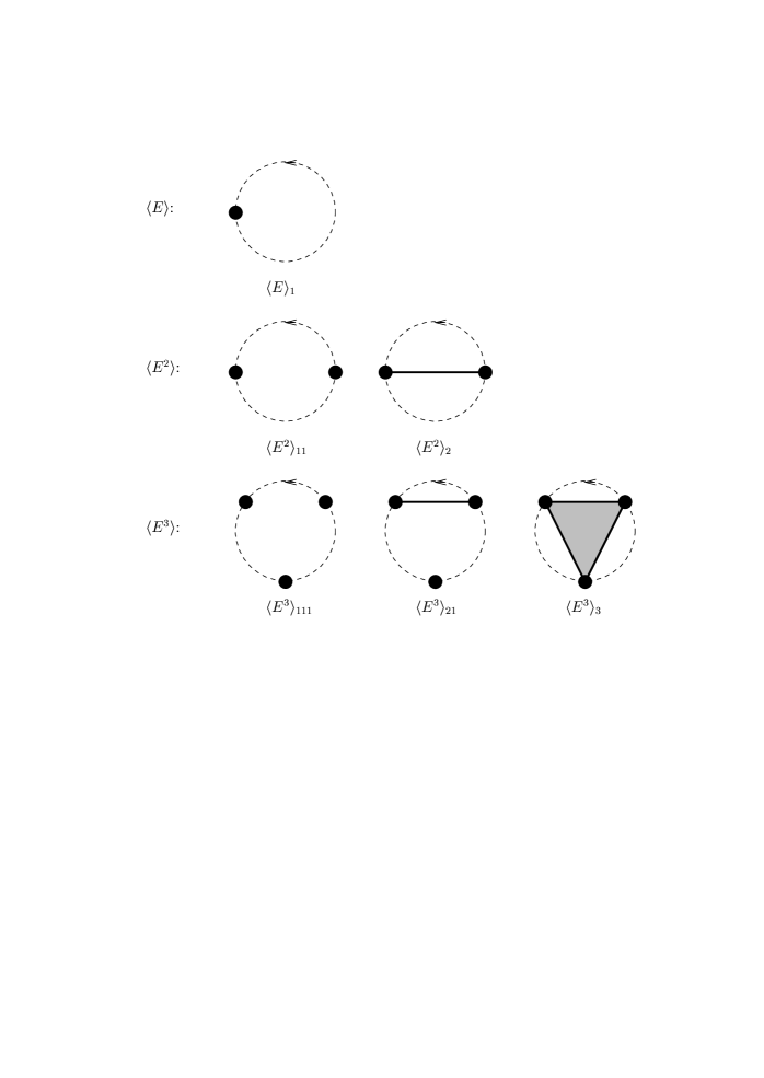
Figure 12: Graphs constituting the first three energy moments $\langle E\rangle,\,\langle E^{2}\rangle$ and $\langle E^{3}\rangle$. Note that the statistical weight is a factor $k!$ higher than the usual combinatorial factor, where $k$ is the order of the moment considered.

We have

$$\langle E\rangle_{1}=f,\quad\langle E^{2}\rangle_{11}=f^{2},\quad\langle E^{3}\rangle_{111}=f^{3},\quad\langle E^{3}\rangle_{12}=3f\,\langle E^{2}\rangle_{2},$$ (41)

which reduces the problem to evaluating $\langle E^{2}\rangle_{2}$ and $\langle E^{3}\rangle_{12}$. These quantities depend on the Landau level index, which we shall indicate in our notation below. The evaluation of $\langle E^{2}\rangle_{2}$ reduces to computing

$$\langle E^{2}\rangle_{2}^{(\nu)}=\frac{f}{\varrho}\int_{-\infty}^{\infty}\frac{\d{\vec{u}}}{2\pi}L_{\nu}^{2}(\,\case 12(1-\case 1\varrho){\vec{u}}^{\,2}\,)\,\exp\left(-\case 12{\vec{u}}^{\,2}\right),$$

where $L_{\nu}$ is the $\nu$’th Laguerre polynomial. Since this is a Gaussian times a polynomial, it is simple to evaluate for the first few $\nu$. We find

$$\begin{array}{cc}& \\ \nu & ⟨E{}^2⟩{}_2{}^{(\nu )}\text{<span class="ltx\_rule" style="width:0.0pt;height:14.2pt;background:black;display:inline-block;"></span>}\\ & \\ & \\ 0& \frac{1}{\varrho }f\text{<span class="ltx\_rule" style="width:0.0pt;height:14.2pt;background:black;display:inline-block;"></span>}\\ 1& \frac{(\varrho -1){}^2+1}{\varrho {}^3}f\text{<span class="ltx\_rule" style="width:0.0pt;height:14.2pt;background:black;display:inline-block;"></span>}\\ 2& \frac{(\varrho -1){}^4+4(\varrho -1){}^2+1}{\varrho {}^5}f\text{<span class="ltx\_rule" style="width:0.0pt;height:14.2pt;background:black;display:inline-block;"></span>}\\ 3& \frac{(\varrho -1){}^6+9(\varrho -1){}^4+9(\varrho -1){}^2+1}{\varrho {}^7}f\text{<span class="ltx\_rule" style="width:0.0pt;height:14.2pt;background:black;display:inline-block;"></span>}\\ & \end{array}Thisfitswithageneralexpression\text{(42)42⟩= f\hspace{0.17em}ϱ ∑ (ϱ-1) ≡, ⟨E2⟩2(ν)= f\hspace{0.17em}ϱ-(2ν+1) ∑k=0ν [ (νk) (ϱ-1)k ]2 ≡fϱe(ν),}where\text{ϱ}\text{\_}\text{^(}\text{ν}\text{)}isarescaled,effectiveformof\text{ϱ},allowingustowritethesecondordermomentforarbitrary\text{ν}inthesameformasthesecondordermomentforthelowestLandaulevel.Weshowinfigure\text{<span class="ltx\_ref ltx\_missing\_label ltx\_font\_italic ltx\_ref\_self">LABEL:fig:Frhoeff</span>}howthisquantityvarieswith\text{ρ}and\text{ν}.\text{Figure 1313Figure 13 13Therescaled,effectivem}$$