STOCHASTIC EFFECTS IN PHYSICAL SYSTEMS

MAXI SAN MIGUEL and RAÚL TORAL
Departamento de Física Interdisciplinar
Instituto Mediterrá neo de Estudios Avanzados IMEDEA (CSIC-UIB)
Campus Universitat de les Illes Balears
E-07071 Palma de Mallorca, Spain
http://www.imedea.uib.es/PhysDept/

1 Introduction

The study of the effects of noise and fluctuations is a well established subject in several different disciplines ranging from pure mathematics (stochastic processes) to physics (fluctuations) and electrical engineering (noise and radiophysics). In traditional statistical physics, fluctuations are of thermal origin giving rise to small departures from a mean value. They tend to zero as one approaches the thermodynamic limit in which different statistical descriptions (different ensembles) become equivalent. Likewise, in more applied contexts fluctuations or noise are usually regarded as small corrections to a deterministic (noise free) behavior that degrades a signal-to-noise ratio or can cause transmission errors. In such framework fluctuations are a correction that can be usually dealt with through some sort of linearization of dynamics around a mean or noise free dynamics. A different point of view about fluctuations emerges, for example, in the study of critical phenomena in the 1970’s. The statistical physics description of these phenomena requires a formulation appropriate for a system dominated by fluctuations and nonlinearities. A linear theory only identifies the existence of a critical point by a divergence of fluctuations.

The renewed interest and activity of the last 15-20 years on stochastic phenomena and their applications is precisely in the context of the study of nonlinear dynamics and instabilities in systems away from equilibrium. This activity has led to some new conceptual developments, applications, and new or rediscovered methodology [1, 2, 3, 4, 5, 6]. Among these we would like to emphasize here two very general aspects. One is the concept that noise need not only be a nuisance that spoils the ”true” and desired behavior of the system, but rather noise might make possible new states and forms of behavior which do not appear in a noise-free limit. These situations might occur when there are mechanisms of noise amplification and/or when noise interacts with nonlinearities or other driving forces of a system. Phenomena like noise sustained spatial structures, noise–induced transitions or stochastic resonance go under this category. A second concept we wish to emphasize is that the physical relevant behavior is not necessarily associated with some ensemble average, but rather with typical stochastic trajectories. It is certainly a trivial mathematical statement that a mean does not always give a typical characterization of a process, but there is a certain tradition in physics (borrowed from equilibrium statistical physics) of focusing on averaged values. A physical intuition or understanding of novel stochastic driven phenomena is in fact gained by the consideration of the individual realizations of the stochastic process. This has important methodological consequences: one needs tools to follow trajectories instead of just looking at averages and probability distributions.

In these lectures we follow an incomplete random walk on the phase space of some of the current concepts, developments and applications of stochastic processes from the point of view of the practitioner physicist and emphasizing examples of the two key ideas outlined above. Section 2 is rather tutorial while the other ones give more a summary and guide to different topics. Some parts of Sect. 2 are rather elementary and can be skipped by anyone with a little experience in stochastic processes. But this section also contains a rather detailed presentation of numerical methods for the simulation of the individual realizations of a stochastic process. It is here important to warn against the naive idea that including noise in the simulation of a nonlinear dynamical problem is just to add some random numbers in any reasonable way. This is particularly important when we want to learn on the physics of the problem following the trajectories. Section 3 deals with one of the important cases of noise amplification, namely the transient decay from unstable states. Key concepts like trajectory dynamics, passage time statistics and mapping of linear into nonlinear stochastic properties are discussed. As an important application of these ideas and methods we discuss properties of laser switch-on viewed as a process of noise amplification. Section 4 is devoted to the analysis of the long–time, stationary, properties of physical systems in the presence of noise. The classification of potential/non–potential systems is succinctly reviewed and the conditions for a system to be potential are precisely stated. We study the general form of the probability distribution function when noise is present. We end with an example borrowed from fluid dynamics, the Küppers–Lortz instability, in which we illustrate the stabilization by noise of a periodic trajectory in a system in which the deterministic dynamics has a contibution which can not be described as relaxation dynamics in a potential. In Section 5 we consider spatially extended systems, described either by ordinary differential equations for the amplitudes of a few spatial modes or by stochastic partial differential equations. Through some specific examples we discuss symmetry breaking by pattern formation and symmetry restoring by noise, the issue of pattern selection in the presence of noise and noise sustained structures in convectively unstable situations. Section 6 reviews the concept of noise–induced transition, distinguishing it from that of noise–induced phase–transition. The difference being, mainly, that noise–induced transitions do not break ergodicity, as we understand a phase transition in the statistical–mechanics sense. We present specific examples of systems displaying one or the other and show that, in general, they can no coexist in the same system.

We should finally make clear that our choice of subjects included in these lectures is rather arbitrary and sometimes dictated by personal contributions. Among many other relevant topics of actual interest which we do not discuss here we could mention, from the methodological point of view, path integral formulations of stochastic processes [6, 7] and from the conceptual point of view stochastic resonance [8] and directed fluxes supported by noise [9]

2 Stochastic Processes

2.1 Basic Concepts

In this first subsection we want to give a quick review of what a stochastic process is from the physical point of view. We will not be too rigorous on the mathematical side. The name “stochastic process” is usually associated with a trajectory which is random enough to demand a probabilistic description. Of course, the paradigmatic example being that of Brownian motion [3, 10, 11, 12, 13]. The botanist Robert Brown discovered in 1827 that particles of pollen in suspension execute random movements which he interpreted initially as some sort of life. It is not so well known that L. Boltzmann knew as early as 1896 the reason for this erratic movement when he wrote “… very small particles in a gas execute motions which result from the fact that the pressure on the surface of the particles may fluctuate” [14]. However, it was A. Einstein in 1905 who successfully presented the correct description of the erratic movement of the Brownian particles [2]. Instead of focusing on the trajectory of a single particle, Einstein derived a probabilistic description valid for an ensemble of Brownian particles. In his description, no attempt is made to follow fully in time the (complicated) trajectory of a Brownian particle. Instead, he introduces the concept of a coarse–grained description, defined by a time scale $\tau$ such that different trajectories separated by a time $\tau$ can be considered independent. No attempt is made to characterize the dynamics at a time scale smaller than this coarse–grain time $\tau$. A second concept, probabilistic in nature, introduced by Einstein is the probability density function (pdf, for short), $f(\vec{\Delta})$, for the distance $\vec{\Delta}$ travelled by the Brownian particle in a time interval $\tau$. $f(\vec{\Delta})$ is defined such that $f(\vec{\Delta})d\vec{\Delta}$ is the probability of having a change in position $\vec{x}$ in the interval $(\vec{\Delta},\vec{\Delta}+d\vec{\Delta})$. From the fact that $f(\vec{\Delta})$ is a pdf it follows the following properties:

$$\begin{array}[]{rcl}f(\vec{\Delta})&\geq&0\\ \int f(\vec{\Delta})d\vec{\Delta}&=&1\end{array}$$ (2.1)

One could invoke the law of large numbers to predict a Gaussian form for $f(\vec{\Delta})$. However, this is not necessary and one only needs to assume the symmetry condition:

$$f(-\vec{\Delta})=f(\vec{\Delta})$$ (2.2)

We consider an ensemble of $N$ Brownian particles. This is characterized by the particle number density $n(\vec{x},t)$, which is such that $n(\vec{x},t)d\vec{x}$ is the number of particles in the volume $(\vec{x},\vec{x}+d\vec{x})$ at time $t$. From the assumption that the trajectories separated a time interval $\tau$ are independent, it follows that the number of particles at location $\vec{x}$ at time $t+\tau$ will be given by the number of particles at location $\vec{x}-\vec{\Delta}$ at time $t$, multiplied by the probability that the particle jumps from $\vec{x}-\vec{\Delta}$ to $\vec{x}$, which is nothing but $f(\vec{\Delta})$, and integrated for all the possible $\vec{\Delta}$ values:

$$n(\vec{x},t+\tau)=\int n(\vec{x}-\vec{\Delta},t)f(\vec{\Delta})d\vec{\Delta}$$ (2.3)

This is the basic evolution equation for the number density $n(x,t)$. By Taylor expanding the above expression, using of the symmetry relation eq.(2.2) and keeping only the lowest non–vanishing order terms, one gets the diffusion equation:

$$\frac{\partial n}{\partial t}=D\nabla^{2}n$$ (2.4)

where the diffusion constant $D$ is given in terms of the second moment of the pdf $f(\vec{\Delta})$ by:

$$D=\frac{1}{2\tau}\int\Delta^{2}f(\vec{\Delta})d\vec{\Delta}=\frac{\langle\Delta^{2}\rangle}{2\tau}$$ (2.5)

If the initial condition is that all particles are located at $\vec{x}=0$, $n(\vec{x},t=0)=N\delta(\vec{x})$, the solution of the diffusion equation is:

$$n(\vec{x},t)=\frac{N}{(4\pi Dt)^{3/2}}{\rm e}^{-x^{2}/4Dt}$$ (2.6)

from where it follows that the average position of the Brownian particle is $0$ and that the average square position increases linearly with time, namely:

$$\begin{array}[]{rcl}\langle\vec{x}(t)\rangle&=&0\\ \langle\vec{x}(t)^{2}\rangle&=&6Dt\end{array}$$ (2.7)

These predictions have been successfully confirmed in experiments and contributed to the acceptance of the atomic theory. The above results are characteristic of stochastic diffusion processes as the ones we will encounter again in other sections (c.f. Sect. 5).

Even though Einstein’s approach was very successful, one has to admit that it is very phenomenological and can not yield, for instance, an explicit expression that allows the calculation of the diffusion constant in terms of microscopic quantities. Langevin (1908) initiated a different treatment which can be considered in some way complementary of the previous one. In his approach, Langevin focused on the trajectory of a single Brownian particle and wrote down Newton’s equation Force=mass $\times$ acceleration. Of course, he knew that the trajectory of the Brownian particle is highly erratic and that would demand a peculiar kind of force. Langevin considered two types of forces acting on the Brownian particle: usual friction forces that, according to Stokes law, would be proportional to the velocity, and a sort of “fluctuating” force $\vec{\xi}(t)$ which represents the “erratic” part of the force coming from the action of the fluid molecules on the Brownian particle. The equation of motion becomes then:

$$m\frac{d\vec{v}}{dt}=-6\pi\eta a\vec{v}+\vec{\xi}$$ (2.8)

$\eta$ is the viscosity coefficient and $a$ is the radius of the (assumed spherical ) Brownian particle. Langevin made two assumptions about the fluctuating force $\vec{\xi}(t)$: that it has mean $0$ and that it is uncorrelated to the actual position of the Brownian particle:

$$\begin{array}[]{rcl}\langle\vec{\xi}(t)\rangle&=&0\\ \langle\vec{x}(t)\cdot\vec{\xi}(t)\rangle&=&\langle\vec{x}(t)\rangle\cdot\langle\vec{\xi}(t)\rangle=0\end{array}$$ (2.9)

Multiplying eq.(2.8) by $\vec{x}$, taking averages with respect to all realizations of the random force $\vec{\xi}(t)$, and using the previous conditions on $\vec{\xi}(t)$ one gets:

$$\frac{m}{2}\frac{d^{2}\;\langle{\vec{x}\;}^{2}\rangle}{dt^{2}}=m\langle{\vec{v}\;}^{2}\rangle-3\pi a\eta\frac{d\;\langle{\vec{x}\;}^{2}\rangle}{dt}$$ (2.10)

Langevin assumed that we are in the regime in which thermal equilibrium between the Brownian particle and the surrounding fluid has been reached. In particular, this implies that, according to the equipartition theorem, the average kinetic energy of the Brownian particle is $\langle m{\vec{v}\;}^{2}/2\rangle=3k_{B}T/2$ ($k_{B}$ is Boltzmann’s constant and $T$ is the fluid temperature). One can now solve very easily eq.(2.10) to find that the particle does not move on the average and that, after some transient time, the asymptotic average square position is given by:

$$\begin{array}[]{rcl}\langle\vec{x}(t)\rangle&=&0\\ \langle{\vec{x}(t)}^{2}\rangle&=&\frac{k_{B}T}{\pi\eta a}t\end{array}$$ (2.11)

This is nothing but Einstein’s diffusion law, but we have now an explicit expression for the diffusion coefficient:

$$D=\frac{k_{B}T}{6\pi\eta a}$$ (2.12)

Langevin’s random force $\vec{\xi}(t)$ and the Brownian particle position $\vec{x}(t)$ are examples of stochastic processes. It is now time we provide a more precise definition of what a stochastic process is. It should be clear that the natural scenario is that of probability theory [15, 16].

Let us consider a probabilistic experiment $E=(S,{\cal F},P)$, where $S$ is a set of possible results, ${\cal F}$ is the $\sigma$–algebra of events, i.e. those subsets of $S$ that are assigned a probability, and the real function $P:{\cal F}\to R$ is a $\sigma$–additive probability. In many occasions, we are interested in a real number associated with the experiment result. We call this a random variable and denote it by $\hat{x}$. In other words, a random variable is an application of the set of results into the set of real numbers

$$\begin{array}[]{rcl}\hat{x}:S&\to&R\\ u&\to&\hat{x}[u]\end{array}$$ (2.13)

In many occasions, the outcome $u$ of the experiment is itself a real number, and we simply define $\hat{x}(u)=u$. In those cases and by abuse of language, the experiment result $u$ is also called a random variable. The probability density function $f(x)$ of the random variable $\hat{x}$ is defined such that $f(x)dx$ is the probability that $\hat{x}$ takes variables in the interval $(x,x+dx)$, namely the probability of the set $\{u\in S~{}|~{}x\leq\hat{x}[u]\leq x+dx\}$.

We now define a stochastic process $\hat{x}(t)$ as a family of random variables depending on some continuous real parameter $t$. It is, then, a family of applications:

$$\begin{array}[]{rcl}\hat{x}(t):S&\to&R\\ u&\to&\hat{x}[t,u]\end{array}$$ (2.14)

Alternatively, for each experiment result $u$ we might now think of $\hat{x}[t,u]\equiv x_{u}(t)$ as a function of the parameter $t$. This is usually the way one considers a stochastic process $\hat{x}(t)$: as a collection of functions $x_{u}(t)$ each one depending of the outcome $u$. In most applications, $t$ is a physical time and $x_{u}(t)$ is a trajectory that depends on the outcome of some probabilistic experiment $S$. In this way, the trajectory itself $x_{u}(t)$ acquires a probabilistic nature.

Arguably, the most well–known example of a stochastic process is that of the random walk [17]. The experiment $S$ is a series of binary results representing, for instance, the outcome of repeatedly tossing a coin: $u=(0,0,0,0,1,1,0,1,1,1,0,1,0,1,0,1,\dots)$ ($1$ means “heads”, $0$ means “tails”). To this outcome we associate a $1$–dimensional real function $x_{u}(t)$ which starts at $x_{u}(0)=0$ and that moves to the left (right) at time $k\tau$ an amount $a$ if the $k$–th result of the tossed coin was 0 (1). Fig. (2.1) shows the “erratic” trajectory for the above result $u$.

Figure 2.1: Random walk trajectory $x_{u}(t)$ associated to the result $u$ of a binary experiment as discussed in the main text.

What does one mean by characterizing a stochastic process? Since it is nothing but a continuous family of random variables, a stochastic process will be completely characterized when we know the joint probability density function for the set $\{\hat{x}(t_{1}),\hat{x}(t_{2}),\dots,\hat{x}(t_{m})\}$, i.e. when we know the function $f(x_{1},\dots,x_{m};t_{1},\dots,t_{m})$ for arbitrary $m$. This function is such that

$$f(x_{1},\dots,x_{m};t_{1},\dots,t_{m})dx_{1}\dots dx_{m}$$ (2.15)

represents the probability that the random variable $\hat{x}(t_{1})$ takes values in the interval $(x_{1},x_{1}+dx_{1})$, the random variable $\hat{x}(t_{2})$ takes values in the interval $(x_{2},x_{2}+dx_{2})$, etc. In a different language, we can say that a complete characterization of the trajectory is obtained by giving the functional probability density function $f([x(t)])$. One has to realize that a complete characterization of a stochastic process implies the knowledge of a function of an arbitrary number of parameters and is very difficult to carry out in practice. In many occasions one is happy if one can find simply the one–time pdf $f(x;t)$ and the two–times pdf $f(x_{1},x_{2};t_{1},t_{2})$. In terms of those, it is possible to compute trajectory averages:

$$\langle\hat{x}(t)^{n}\rangle=\int_{-\infty}^{\infty}dx\;x^{n}f(x;t)$$ (2.16)

and time correlations:

$$\langle\hat{x}(t_{1})\hat{x}(t_{2})\rangle=\int_{-\infty}^{\infty}dx_{1}\;dx_{2}\;x_{1}x_{2}f(x_{1},x_{2};t_{1},t_{2})$$ (2.17)

It is important to understand that the averages $\langle\dots\rangle$ are taken with respect to all the possible realizations of the stochastic process $\hat{x}(t)$, i.e. with respect to all the possible outcomes $u$ of the experiment. Every outcome $u$ gives rise to a different trajectory $x_{u}(t)$. The different trajectories are usually called “realizations” of the stochastic process $\hat{x}(t)$. An alternative way of understanding the previous averages is by performing the experiment a (preferably large) number of times $M$ to obtain the results $u_{i}$, $i=1,\dots,M$, and the different trajectory realizations $x_{u_{i}}(t)$. The averages can then be performed by averaging over the different trajectories as:

$$\langle\hat{x}(t)\rangle=\frac{1}{M}\sum_{i=1}^{M}x_{u_{i}}(t)$$ (2.18)

and similar expressions for other averages.

In two very interesting cases does the knowledge of $f(x;t)$ and $f(x_{1},x_{2};t_{1},t_{2})$ imply the knowledge of the complete pdf $f(x_{1},\dots,x_{m};t_{1},\dots,t_{m})$ for arbitrary $m$: (i) Complete time independence and (ii) Markov process. In a complete time–independent process, the random variables at different times are independent and we are able to write:

$$f(x_{1},\dots,x_{m};t_{1},\dots,t_{m})=f(x_{1};t_{1})f(x_{2};t_{2})\dots f(x_{m};t_{m})$$ (2.19)

In the case of a so–called Markov process, the rather general conditional probability

$$f(x_{m};t_{m}|x_{1},\dots,x_{m-1};t_{1},\dots,t_{m-1})\equiv\frac{f(x_{1},\dots,x_{m};t_{1},\dots,t_{m})}{f(x_{1},\dots,x_{m-1};t_{1},\dots,t_{m-1})}$$ (2.20)

is equal to the two–times conditional probability

$$f(x_{m};t_{m}|x_{m-1};t_{m-1})\equiv\frac{f(x_{m-1},x_{m};t_{m-1},t_{m})}{f(x_{m-1};t_{m-1})}$$ (2.21)

for all times $t_{m}>t_{m-1}>\dots>t_{1}$. Loosely speaking, the Markov property means that the probability of a future event depends only on the present state of the system and not on the way it reached its present situation. In this case one can compute the $m$–times pdf as:

$$\begin{array}[]{rcl}&&f(x_{1},\dots,x_{m};t_{1},\dots,t_{m})=\\ &&f(x_{m};t_{m}|x_{m-1};t_{m-1})f(x_{m-1};t_{m-1}|x_{m-2};t_{m-2})\dots f(x_{2};t_{2}|x_{1};t_{1})f(x_{1};t_{1})\end{array}$$ (2.22)

The random walk is an example of a Markov process, since the probability of having a particular value of the position at time $(k+1)\tau$ depends only on the particle location at time $k\tau$ and not on the way it got to this location.

Another important category is that of Gaussian processes [18] for which there is an explicit form for the $m$–times pdf, namely:

$$f(x_{1},\dots,x_{m};t_{1},\dots,t_{m})=\sqrt{\frac{|S|}{(2\pi)^{m}}}\exp{\left[-\frac{1}{2}\sum_{i,j=1}^{m}(x_{i}-b_{i})S_{ij}(x_{j}-b_{j})\right]}$$ (2.23)

where the parameters of this expression can be related to mean values of the random variables as:

$$\begin{array}[]{rcl}b_{i}&=&\langle\hat{x}(t_{i})\rangle\\ (S^{-1})_{ij}&=&\langle\hat{x}(t_{i})\hat{x}(t_{j})\rangle-\langle\hat{x}(t_{i})\rangle\langle\hat{x}(t_{j})\rangle\end{array}$$ (2.24)

As a consequence, one very rarely writes out the above form for the pdf, and rather characterizes the Gaussian process by giving the mean value $\langle\hat{x}(t)\rangle$ and the correlation function $\langle\hat{x}(t)\hat{x}(t^{\prime})\rangle$. From the many properties valid for Gaussian processes, we mention that a linear combination of Gaussian processes is also a Gaussian process.

2.2 Stochastic Differential Equations

A stochastic differential equation (SDE) is a differential equation which contains a stochastic process $\hat{\xi}(t)$:

$$\frac{d\hat{x}(t)}{dt}=G(\hat{x}(t),t,\hat{\xi}(t))$$ (2.25)

Let us explain a little further what is meant by the previous notation. $G$ is a given 3–variable real function. $\hat{\xi}(t)$ is a stochastic process: a family of functions $\xi_{u}(t)$ depending on the outcome $u$ of some experiment $S$. As a consequence a SDE is not a single differential equation but rather a family of ordinary differential equations, a different one for each outcome $u$ of the experiment $S$:

$$\frac{dx_{u}(t)}{dt}=G(x_{u}(t),t,\xi_{u}(t))$$ (2.26)

Therefore, the family of solutions $x_{u}(t)$ of these differential equations, for different outcomes $u$, constitute a stochastic process $\hat{x}(t)$. We can say that for each realization $\xi_{u}(t)$ of the stochastic process $\hat{\xi}$, corresponds a realization $x_{u}(t)$ of the stochastic process $\hat{x}$. The solution $\hat{x}$ becomes then a functional of the process $\hat{\xi}$. To “solve” a SDE means to characterize completely the stochastic process $\hat{x}(t)$, i.e. to give the $m$–times pdf $f(x_{1},\dots,x_{m};t_{1},\dots,t_{m})$. Again, this is in general a rather difficult task and sometimes one focuses only on the evolution of the moments $\langle\hat{x}(t)^{n}\rangle$ and the correlation function $\langle\hat{x}(t_{1})\hat{x}(t_{2})\rangle$.

When the stochastic process $\hat{\xi}(t)$ appears linearly one talks about a Langevin equation. Its general form being:

$$\frac{dx}{dt}=q(x,t)+g(x,t)\xi(t)$$ (2.27)

(from now on, and to simplify notation, the “hats” will be dropped from the stochastic processes). In this case, $\xi(t)$ is usually referred to as the “noise” term. A word whose origin comes from the random “noise” one can actually hear in electric circuits. Still another notation concept: if the function $g(x,t)$ is constant, one talks about additive noise, otherwise, the noise is said to be multiplicative. Finally, $q(x,t)$ is usually referred to as the “drift” term, whereas $g(x,t)$ is the “diffusion” term (a notation which is more commonly used in the context of the Fokker–Planck equation, see later).

Of course, we have already encountered a Langevin SDE, this is nothing but Langevin’s equation for the Brownian particle, equation (2.8). In this example, the stochastic noise was the random force acting upon the Brownian particle. The “experiment” that gives rise to a different force is the particular position and velocities of the fluid molecules surrounding the Brownian particle. The movements of these particles are so erratic and unpredictable that we assume a probabilistic description of their effects upon the Brownian particle.

We will now characterize the process $\xi(t)$ that appears in the Langevin equation for the Brownian particle. We will be less rigorous here in our approach and, in fact, we will be nothing but rigorous at the end! but still we hope that we can give a manageable definition of the stochastic force $\xi(t)$. We first need to define the stochastic Wiener process $W(t)$. This is obtained as a suitable limit of the random walk process [16]. The probability that the walker is at location $x=r\,a$ after time $t=n\,\tau$ can be expressed in terms of the binomial distribution:

$$P(x(n\tau)=ra)={n\choose{\frac{n+r}{2}}}2^{-n}$$ (2.28)

From where it follows:

$$\begin{array}[]{rcl}\langle x(n\tau)\rangle&=&0\\ \langle x(n\tau)^{2}\rangle&=&na^{2}\\ \end{array}$$ (2.29)

For $n\gg 1$ we can use the asymptotic result (de Moivre–Laplace theorem) that states that the binomial distribution can be replaced by a Gaussian distribution:

$$P(x(n\tau)\leq ra)=\frac{1}{2}+{\rm erf}\left(\frac{r}{\sqrt{n}}\right)$$ (2.30)

(${\rm erf}(x)$ is the error function [19]). We now take the continuum limit defined by:

$$\begin{array}[]{lr}n\to\infty,~{}\tau\to 0&n\tau=t\\ r\to\infty,~{}a\to 0&ra=s\\ &a^{2}/\tau=1\end{array}$$ (2.31)

with finite $t$ and $s$. In this limit the random walk process is called the Wiener process $W(t)$ and equation (2.30) tends to:

$$P(W(t)\leq s)=\frac{1}{2}+{\rm erf}\left(\frac{s}{\sqrt{t}}\right)$$ (2.32)

which is the probability distribution function of a Gaussian variable of zero mean and variance $t$. The corresponding one–time probability density function for the Wiener process is:

$$f(W;t)=\frac{1}{\sqrt{2\pi t}}\exp{(-\frac{W^{2}}{2t})}$$ (2.33)

The Wiener process is a Markovian (since the random walk is Markovian) Gaussian process. As every Gaussian process it can be fully characterized by giving the one–time mean value and the two–times correlation function. These are easily computed as:

$$\begin{array}[]{rcl}\langle W(t)\rangle&=&0\\ \langle W(t)^{2}\rangle&=&t\\ \langle W(t_{1})W(t_{2})\rangle&=&\min(t_{1},t_{2})\\ \end{array}$$ (2.34)

A typical realization of the Wiener process is given in Fig. (2.2).

Figure 2.2: A typical realization of the Wiener process done by generating a random walk with a large number of steps.

The Wiener process is continuous but it does not have first derivative. In fact it is a fractal of Hausdorff dimension $2$ [20].

We will define now the white–noise random process as the derivative of the Wiener process. Since we just said that the Wiener process does not have a derivative, it is not surprising that the resulting function is a rather peculiar function. The trick is to perform the derivative before the continuum limit (2.31) is taken. If $x(t)$ is the random walk process, we define the stochastic process $w_{\epsilon}(t)$ as:

$$w_{\epsilon}(t)=\frac{x(t+\epsilon)-x(t)}{\epsilon}$$ (2.35)

$w_{\epsilon}(t)$ is a Gaussian process since it is a linear combination of Gaussian processes. Therefore, it is sufficiently defined by its mean value and correlations:

$$\begin{array}[]{rcl}\langle w_{\epsilon}(t)\rangle&=&0\\ \langle w_{\epsilon}(t_{1})w_{\epsilon}(t_{2})\rangle&=&\left\{{\begin{array}[]{lcr}&0&{\rm if}~{}t_{1}-t_{2}<-\epsilon\\ &a^{2}/(\tau\epsilon)(1+(t_{1}-t_{2})/\epsilon)&{\rm if}~{}-\epsilon\leq t_{1}-t_{2}\leq 0\\ &a^{2}/(\tau\epsilon)(1-(t_{1}-t_{2})/\epsilon)&{\rm if}~{}0\leq t_{1}-t_{2}\leq\epsilon\\ &0&{\rm if}~{}t_{1}-t_{2}>\epsilon\end{array}}\right.\end{array}$$ (2.36)

which is best understood by the plot in Fig. (2.3).

Figure 2.3: Correlation function for the derivative of the random walk process, equation (2.36).

If we let now $\epsilon\to 0$ the process $w(t)=\lim_{\epsilon\to 0}w_{\epsilon}(t)$ becomes the derivative of the random walk process. The correlation function (2.36) becomes a delta function $(a^{2}/\tau)\delta(t_{1}-t_{2})$. If we take now the limit defined in eqs.(2.31) the random walk process tends to the Wiener process $W(t)$ and the derivative process $w(t)$ tends to $\xi_{w}(t)$: the white–noise process. Intuitively, the white–noise represents a series of independent pulses acting on a very small time scale but of high intensity, such that their effect is finite. The white noise can be considered the ideal limit of a physical stochastic process in the limit of very small correlation time $\tau$. Formally, the white noise is defined as a Markovian, Gaussian process of mean value and correlations given by:

$$\begin{array}[]{rcl}\langle\xi_{w}(t)\rangle&=&0\\ \langle\xi_{w}(t_{1})\xi_{w}(t_{2})\rangle&=&\delta(t_{1}-t_{2})\end{array}$$ (2.37)

and can be considered the derivative of the Wiener process:

$$\xi_{w}(t)=\frac{dW(t)}{dt}$$ (2.38)

All this lack of mathematical rigor leads to some problems of interpretation. For instance, when in a SDE the white–noise appears multiplicatively, the resulting process $x(t)$ will be, in general, a non continuous function of time. When this happens, there is an ambiguity in some mathematical expressions. Giving a sense to those a priori undefined expressions constitutes a matter of sheer definition. The most widely used interpretations are those of Itô and Stratonovich [1, 2]. To make a long story short, we can summarize both interpretations as follows: when in a calculation we are faced with an integral

$$\int_{t}^{t+h}ds\;g(x(s))\xi_{w}(s)$$ (2.39)

to be computed in the limit $h\to 0$, Itô interprets this as:

$$g(x(t))\int_{t}^{t+h}ds\;\xi_{w}(s)=g(x(t))[W(t+h)-W(t)]$$ (2.40)

and Stratonovich as:

$$\frac{g(x(t))+g(x(t+h))}{2}\int_{t}^{t+h}ds\;\xi_{w}(s)=\frac{g(x(t))+g(x(t+h))}{2}[W(t+h)-W(t)]$$ (2.41)

Although there was much arguing in the past to which is the “correct” interpretation, it is clear now that it is just a matter of convention. This is to say, the Langevin SDE (2.27) is not completely defined unless we define what do we interpret when we encounter expressions such as eq.(2.39). In some sense, it is related to the problem of defining the following expression involving the Dirac–delta function:

$$\int_{0}^{\infty}dt\;\delta(t)$$ (2.42)

This can be defined as equal to $1$ (equivalent to the Itô rule) or to $1/2$ (Stratonovich). Both integration rules give different answers and one should specify from the beginning which is the interpretation one is using. The Stratonovich rule turns out to be more “natural” for physical problems because it is the one that commutes with the limit (2.31). Unless otherwise stated, we will follow in general the Stratonovich interpretation. Moreover, the Stratonovich interpretation allows us to use the familiar rules of calculus, such as change of variables in an integration, etc. The use of the Itô rules leads to relations in which some of the familiar expressions of ordinary calculus are not valid and one needs to be a little bit more cautious when not used to it. A consequence of the Itô interpretation is the simple result $\langle x(t)\xi_{w}(t)\rangle=0$ which is not valid in the Stratonovich interpretation (see later Eq. (2.56)). However, there is a simple relation between the results one obtains in the two interpretations. The rule is that the SDE

$$\frac{dx}{dt}=q(x)+g(x)\xi_{w}(t)$$ (2.43)

in the Itô sense, is equivalent to the SDE:

$$\frac{dx}{dt}=q(x)-\frac{1}{2}g(x)g^{\prime}(x)+g(x)\xi_{w}(t)$$ (2.44)

in the Stratonovich sense. This rule allows to easily translate the results one obtains in both interpretations. Both interpretations coincide for additive noise.

The white noise process is nothing but a physical idealization that leads to some mathematical simplifications. For instance, it can be proven that the solution $x(t)$ of the Langevin equation (2.43) is a Markov process if $\xi(t)$ is a white–noise process. In any physical process, however, there will be a finite correlation time $\tau$ for the noise variables. A widely used process that incorporates the concept of a finite correlation time is the Ornstein–Uhlenbeck noise, $\xi_{OU}$ [1]. This is formally defined as a Gaussian Markov process characterized by:

$$\begin{array}[]{rcl}\langle\xi_{OU}(t)\rangle&=&0\\ \langle\xi_{OU}(t)\xi_{OU}(t^{\prime})\rangle&=&\frac{1}{2\tau}{\rm e}^{-|t-t^{\prime}|/\tau}\end{array}$$ (2.45)

Several comments are in order:
(i) The OU–noise has a non zero correlation time $\tau$ meaning that values of the noise at different times are not independent random variables. This is a more faithful representation of physical reality than the white–noise limit.
(ii) In the limit $\tau\to 0$ the white noise limit $\xi_{w}(t)$ (with the correlations given in eq.(2.37)) is recovered and the corresponding SDE’s are to be interpreted in the Stratonovich sense.
(iii) The OU–noise is, up to a change of variables, the only Gaussian, Markov, stationary process.
(iv) The OU-noise is the solution of the SDE:

$$\frac{d\xi_{OU}}{dt}=-\frac{1}{\tau}\xi_{OU}(t)+\frac{1}{\tau}\xi_{w}(t)$$ (2.46)

with the initial condition that $\xi_{OU}(0)$ is a Gaussian random variable of mean $0$ and variance $(2\tau)^{-1}$.

2.3 The Fokker–Planck Equation

We will find now an equation for the one–time pdf for a stochastic process which arises as a solution of a SDE with Gaussian white noise. This is called the Fokker–Planck equation [3]. It is the equivalent of Einstein’s description which focuses on probabilities rather than in trajectories as in the Langevin approach. More precisely, we want to find an equation for the one–time pdf $f(x,t)$ of a stochastic process governed by the SDE of the Langevin form:

$$\frac{dx}{dt}=q(x)+g(x)\xi_{w}(t)$$ (2.47)

with the white–noise defined in eq.(2.37). This is to be understood in the Stratonovich interpretation. To find an equation for the probability density function $f(x;t)$ we will rely upon functional methods [21, 22]. Let us consider first the corresponding deterministic initial value problem:

$$\begin{array}[]{rcl}\dot{x}&=&q(x)\\ x(t=0)&=&x_{0}\end{array}$$ (2.48)

The solution of this equation is a (deterministic) function $x(t,x_{0})$. We can think of $x(t)$ as a random variable whose probability density function $\rho(x;t)$ is a delta–function:

$$\rho(x;t)=\delta(x-x(t,x_{0}))$$ (2.49)

We can now turn $x(t)$ very easily into a stochastic process by simply letting the initial condition $x_{0}$ become a random variable. For each possible value of $x_{0}$ we have a different solution $x(t,x_{0})$, i.e. a random process. In this case the probability density function $\rho(x,t)$ is obtained by averaging the above pdf over the distribution of initial conditions:

$$\rho(x;t)=\langle\delta(x-x(t,x_{0}))\rangle_{x_{0}}$$ (2.50)

But it is well known from mechanics that the density $\rho(x;t)$ satisfies Liouville’s continuity equation [23]:

$$\frac{\partial\rho}{\partial t}+\frac{\partial}{\partial x}(\dot{x}\rho)=0$$ (2.51)

or, using, eq.(2.48):

$$\frac{\partial\rho}{\partial t}=-\frac{\partial}{\partial x}[q(x)\rho]$$ (2.52)

If we consider now the full SDE (2.47) we can repeat the above argument for a given realization of the noise term. The probability density function $f(x;t)$ will be the average of $\rho(x;t)$ with respect to the noise distribution:

$$f(x;t)=\langle\rho(x;t)\rangle_{\xi_{w}}=\langle\delta(x-x(t,x_{0}))\rangle_{x_{0},\xi_{w}}$$ (2.53)

where $\rho$ satisfies the Liouville equation (2.51) and, after substitution of (2.47):

$$\frac{\partial\rho}{\partial t}=-\frac{\partial}{\partial x}[(q(x)+g(x)\xi(t))\rho]$$ (2.54)

By taking averages over the noise term we get:

$$\frac{\partial f}{\partial t}=-\frac{\partial}{\partial x}[q(x)f]-\frac{\partial}{\partial x}[g(x)\langle\xi(t)\rho(x,[\xi(t)])\rangle]$$ (2.55)

The averages are done by using Novikov’s theorem [24]:

$$\langle\xi(t)\rho([\xi(t)])\rangle=\int_{0}^{t}ds\;\langle\xi(t)\xi(s)\rangle\left\langle\frac{\delta\rho}{\delta\xi(s)}\right\rangle$$ (2.56)

which applies to any functional $\rho([\xi(t)])$ of a Gaussian process $\xi(t)$ of zero mean, $\langle\xi(t)\rangle=0$. For the white–noise process:

$$\langle\xi_{w}(t)\rho([\xi_{w}(t)])\rangle=\frac{1}{2}\left\langle\frac{\delta\rho}{\delta\xi_{w}(s)}\right\rangle_{s=t}$$ (2.57)

By using the functional calculus, this can be computed as:

$$\left\langle\frac{\delta\rho}{\delta\xi_{w}(s)}\right\rangle_{s=t}=\left\langle\frac{\delta x(t)}{\delta\xi_{w}(s)}\right|_{s=t}\left.\frac{\delta\rho}{\delta x(t)}\right\rangle=-\frac{\partial}{\partial x}\left\langle\frac{\delta x(t)}{\delta\xi_{w}(s)}\right|_{s=t}\rho\rangle$$ (2.58)

By using the formal solution of eq.(2.47):

$$x(t)=x_{0}+\int_{0}^{t}ds\;q(x(s))+\int_{0}^{t}ds\;g(x(s))\xi_{w}(s)$$ (2.59)

we get:

$$\left.\frac{\delta x(t)}{\delta\xi_{w}(s)}\right|_{s=t}=g(x(t))$$ (2.60)

and

$$\left\langle\frac{\delta\rho}{\delta\xi_{w}(s)}\right\rangle_{s=t}=-\frac{\partial}{\partial x}[g(x)\langle\rho\rangle]=-\frac{\partial}{\partial x}[g(x)f]$$ (2.61)

By substitution in (2.57) and (2.55) we get, finally, the Fokker–Planck equation for the probability density function:

$$\frac{\partial f}{\partial t}=-\frac{\partial}{\partial x}[q(x)f]+\frac{1}{2}\frac{\partial}{\partial x}[g(x)\frac{\partial}{\partial x}[g(x)f]]$$ (2.62)

The above functional method to derive the Fokker–Planck equation from the Langevin equation is very powerful and can be extended to other situations such as the multivariate case and SDE with colored (Ornstein-Uhlenbeck) noise. For colored noise the problem is nonmarkovian and no exact Fokker-Planck equation can be derived for the probability density. Still one can obtain different approximate equations for the probability density and for the two-time probability density [25].

Much work has been devoted to finding solutions to the Fokker–Planck equation. For the stationary equation, $\partial P/\partial t=0$, the solution can be always reduced to quadratures in the one–variable case. The multivariate equation is more complicated and some aspects are discussed in Sect. 4.2.

2.4 Numerical generation of trajectories

In the Langevin’s approach to stochastic processes, a great deal of relevance is given to the trajectories. It is of great importance, therefore, when given a SDE of the form of eq.(2.25), to be able to generate representative trajectories. This is to say: to generate the functions $x_{u}(t)$ for different outcomes $u$ of the experiment. If we generate, say $M$ results $u_{i}$, the averages could be obtained by performing explicitly the ensemble average as indicated in equation (2.18).

We now explain the basic algorithms to generate trajectories starting from a SDE of the Langevin form [21, 26, 27, 28].

2.4.1 The white noise case: Basic algorithms

Euler’s algorithm is by far the simplest one can devise to generate trajectories. We will explain it by using a simple example. Let us consider the SDE:

$$\dot{x}(t)=f(t)+\xi_{w}(t)$$ (2.63)

If fact, this equation is so simple that it can be solved exactly. For a given realization of the noise term, the solution is:

$$x(t)=x(0)+\int_{0}^{t}f(s)\,ds+\int_{0}^{t}\xi_{w}(s)\,ds\equiv x(0)+F(t)+W(t)$$ (2.64)

$W(t)$ is the Wiener process. Hence, we conclude that the stochastic process $x(t)$ is Gaussian and is completely characterized by:

$$\begin{array}[]{rcl}\langle x(t)\rangle&=&x(0)+F(t)\\ \langle x(t)x(t^{\prime})\rangle&=&(x(0)+F(t))(x(0)+F(t^{\prime}))+\min(t,t^{\prime})\end{array}$$ (2.65)

However, let us forget for the moment being that we can solve the SDE and focus on a numerical solution in which we generate trajectories. We do so by obtaining $x(t)$ at discrete time intervals:

$$\begin{array}[]{lll}x(t+h)&=&x(t)+\int_{t}^{t+h}\dot{x}(s)\,ds\\ &=&x(t)+\int_{t}^{t+h}f(s)\,ds+\int_{t}^{t+h}\xi_{w}(s)\,ds\\ &\equiv&x(t)+f_{h}(t)+w_{h}(t)\end{array}$$ (2.66)

here, $w_{h}(t)=W(t+h)-W(t)$ is the difference of the Wiener process at two different times and it is, therefore, a Gaussian process. $w_{h}(t)$ can be characterized by giving the mean and correlations:

$$\langle w_{h}(t)\rangle=\int_{t}^{t+h}\langle\xi_{w}(s)\rangle\,ds=0$$ (2.67)

$$\begin{array}[]{lll}\langle w_{h}(t)w_{h}(t^{\prime})\rangle&=&\int_{t}^{t+h}\,ds\int_{t^{\prime}}^{t^{\prime}+h}\,du\langle\xi_{w}(s)\xi_{w}(u)\rangle\\ &=&\int_{t}^{t+h}\,ds\int_{t^{\prime}}^{t^{\prime}+h}\,du\delta(s-u)\end{array}$$ (2.68)

The integral is an easy exercise on $\delta$ function integration: we can assume, without loss of generality that $t^{\prime}>t$. If $t^{\prime}>t+h$ the integral is $0$ since there is no overlap in the integration intervals and the delta function vanishes. If $t\leq t^{\prime}<t+h$ the double integral equals the length of the overlap interval:

$$\langle w_{h}(t)w_{h}(t^{\prime})\rangle=\int_{t^{\prime}}^{t+h}\,ds=t-t^{\prime}+h$$ (2.69)

In particular, we notice the relation

$$\langle w_{h}(t)^{2}\rangle=h$$ (2.70)

It is important to realize that, if $t_{i}=i~{}h$, $t_{j}=j~{}h$ are the times appearing in the recurrence relation eq.(2.66), we have:

$$\langle w_{h}(t_{i})w_{h}(t_{j})\rangle=h\delta_{ij}$$ (2.71)

We introduce now a set of independent Gaussian random variables $u(t)$ defined only for the discrete set of recurrence times, $t=0$, $h$, $2h$, $\dots$, of mean zero and variance one:

$$\begin{array}[]{rcl}\langle u(t)\rangle=0&,&\langle u(t^{2})\rangle=1\\ \langle u(t)u(t^{\prime})\rangle=0&,&t\neq t^{\prime}\end{array}$$ (2.72)

There is a vast amount of literature devoted to the question of generation of random numbers with a given distribution [29, 30, 31, 32]. The set of numbers $u(t)$ can be generated by any of the standard methods available. One of the most widely used is the Box–Muller–Wiener algorithm: if $r_{1}$ and $r_{2}$ are random numbers uniformly distributed in the interval $(0,1)$ the transformation:

$$\begin{array}[]{rcl}g_{1}&=&\sqrt{-2\ln(r_{1})}\cos(2\pi r_{2})\\ g_{2}&=&\sqrt{-2\ln(r_{1})}\sin(2\pi r_{2})\end{array}$$ (2.73)

returns for $g_{1}$, $g_{2}$ two Gaussian distributed random numbers of mean zero and variance one. This, or other appropriate algorithm, can be used to generated the set of Gaussian variables $u(t)$. In terms of this set of variables we can write:

$$w_{h}(t)=h^{1/2}\,u(t)$$ (2.74)

Finally, the recurrence relation that generates trajectories of eq.(2.63) is the Euler algorithm:

$$\begin{array}[]{rcl}x(t=0)&=&x_{0}\\ x(t+h)&=&x(t)+f_{h}(t)+h^{1/2}\,u(t)\end{array}$$ (2.75)

For the deterministic contribution we can approximate $f_{h}(t)\approx hf(t)$ from where it follows that the deterministic contribution is of order $h^{1}$ and successive contributions go as $h^{2}$, $h^{3}$, etc. On the other hand, the contribution coming from the white noise term is of order $h^{1/2}$ and, in general, successive contribution will scale as $h^{1}$, $h^{3/2}$, etc.

With the experience we have got by solving the previous simple example, let us now tackle a more complicated case. Let us consider the following SDE:

$$\dot{x}(t)=q(x)+g(x)\xi_{w}(t)$$ (2.76)

At this step, one might ask why, given that for a particular realization of the noise term the equation becomes an ordinary differential equation (ode), we need special methods to deal with this kind of equations. The answer lies in the fact that all the methods developed to deal with ODE’s assume that the functions appearing in the equation have some degree of “well–behaveness”. For instance, they are differentiable to some required order. This is simply not the case for the white–noise functions. Even for a single realization of the white–noise term, the function is highly irregular, not differentiable and, in our non rigorous treatment, is nothing but a series of delta–functions spread all over the real axis. This is the only reason why we can not use the well known predictor–corrector, Runge–Kutta and all the like methods without suitable modifications. If our SDE happened to have smooth functions as random processes we could certainly implement all these wonderful methods and use all the standard and very effective routines available! However, this is usually not the case: the stochastic contribution is a non analytical function and we must resource to new and generally more complicated algorithms. The answer lies in integral algorithms: whereas the derivatives of the white–noise function are not well defined, the integrals are (the first integral is the Wiener process, which is a continuous function). We look for a recursion relation by integration of the SDE (2.76):

$$x(t+h)-x(t)=\int_{t}^{t+h}q(x(s))\,ds+\int_{t}^{t+h}g(x(s))\xi_{w}(s)\,ds$$ (2.77)

Now we assume that the functions $q(x)$ and $g(x)$ are differentiable functions and we Taylor–expand $q(x(s))$ and $g(x(s))$ around $x=x(t)$:

$$q(x(s))=q(x(t))+\left.\frac{dq}{dx}\right|_{x(t)}\left(x(s)-x(t)\right)+O[\left(x(s)-x(t)\right)^{2}]$$ (2.78)

$$g(x(s))=g(x(t))+\left.\frac{dg}{dx}\right|_{x(t)}\left(x(s)-x(t)\right)+O[\left(x(s)-x(t)\right)^{2}]$$ (2.79)

Substitution of the lowest possible order of these expansions, i.e., $q(x(s))=q(x(t)),~{}g(x(s))=g(x(t))$ in eq.(2.77) yields:

$$x(t+h)-x(t)=hq(x(t))+hO[x(s)-x(t)]+w_{h}(t)g(x(t))+w_{h}(t)O[x(s)-x(t)]$$ (2.80)

where, as in the simple previous example,

$$w_{h}(t)=\int_{t}^{t+h}\,ds\;\xi_{w}(s)=h^{1/2}\,u(t)$$ (2.81)

is of order $h^{1/2}$. To the lowest order ($h^{1/2}$) we have:

$$x(s)-x(t)=g(x(t))\int_{t}^{s}\,dv\;\xi_{w}(v)=O[h^{1/2}]$$ (2.82)

Therefore we need to go one step further in the Taylor expansion of the function $g(x(s))$ and the next–order contribution to (2.77) is:

$$\begin{array}[]{rcl}&&g^{\prime}(x(t))\int_{t}^{t+h}\,ds\;(x(s)-x(t))\xi_{w}(s)+O[x(s)-x(t)]^{2}w_{h}(t)=\\ &&g^{\prime}(x(t))g(x(t))\int_{t}^{t+h}\,ds\;\int_{t}^{s}\,dv\;\xi_{w}(s)\xi_{w}(v)+O[h^{3/2}]\end{array}$$ (2.83)

The double integral can be easily done by changing the integration order:

$$\int_{t}^{t+h}ds\int_{t}^{s}dv\;\xi_{w}(s)\xi_{w}(v)=\int_{t}^{t+h}dv\int_{v}^{t+h}ds\;\xi_{w}(s)\xi_{w}(v)=\int_{t}^{t+h}ds\int_{s}^{t+h}dv\;\xi_{w}(s)\xi_{w}(v)$$ (2.84)

where to go from the first expression to the second we have exchanged the integration order and, to go from the second to the third, we have exchanged the variables names $v\leftrightarrow s$. Since the first and third integrals are equal they also equal one half of their sum, and the previous integrals can be replaced by:

$$\frac{1}{2}\int_{t}^{t+h}dv\int_{t}^{t+h}ds\;\xi_{w}(s)\xi_{w}(v)=\frac{1}{2}\int_{t}^{t+h}ds\;\xi_{w}(s)\int_{t}^{t+h}dv\;\xi_{w}(v)=\frac{1}{2}\left[w_{h}(t)\right]^{2}$$ (2.85)

Putting all the bits together, we arrive at the desired result which is :

$$x(t+h)=x(t)+h^{1/2}g(x(t))u(t)+h\left[q(x(t))+\frac{1}{2}g(x(t))g^{\prime}(x(t))u(t)^{2}\right]+O[h^{3/2}]$$ (2.86)

This recurrence relation is known in the literature as Milshtein method [21, 33]. If the noise is additive: $g^{\prime}(x)=0$, then the resulting algorithm is called the Euler algorithm:

$$x(t+h)=x(t)+hq(x(t))+g(x(t))h^{1/2}u(t)+O[h^{3/2}]$$ (2.87)

Sometimes, though, the name “Euler algorithm” is also given to a modification of the Milshtein algorithm in which the $u(t)^{2}$ term is replaced by its mean value: $\langle u(t)^{2}\rangle=1$:

$$x(t+h)=x(t)+g(x(t))h^{1/2}u(t)+h[q(x(t))+\frac{1}{2}g(x(t))g^{\prime}(x(t))]+O[h^{3/2}]$$ (2.88)

This “Euler algorithm” is the one appearing naturally when one does the numerical integration of the SDE in the Itô formalism, although at this level it has to be considered just as an approximation, unnecessary, to the Milshtein method.

In the previous expressions, the correction to the recurrence algorithm is said to be of order $O[h^{3/2}]$. Let us explain a little further what is meant by this expression. We use the following notation: we call $\bar{x}(t)$ the values obtained from the numerical integration following the Milshtein method:

$$\bar{x}(t+h)=x(t)+h^{1/2}g(x(t))u(t)+h\left[q(x(t))+\frac{1}{2}g(x(t))g^{\prime}(x(t))u(t)^{2}\right]$$ (2.89)

and we want to compare $\bar{x}(t+h)$ with the exact value $x(t+h)$ which is obtained by exact integration of the differential equation starting from $x(t)$. What we have proven is that the mean–square error (averaged over noise realizations) for the trajectories starting at $x(t)$ is of order $O[h^{3}]$:

$$\langle(\bar{x}(t+h)-x(t+h))^{2}\rangle=O[h^{3}]$$ (2.90)

One says that the Milshtein algorithm has a convergence for the trajectories in mean square of order $h^{3}$. This is related, but not the same, as the order of convergence of the $n$–th order moment, $D_{n}(h)$, which is defined as:

$$D_{n}(h)\equiv\langle\bar{x}(t+h)^{n}\rangle-\langle x(t+h)^{n}\rangle$$ (2.91)

the averages are done starting from a given $x(t)$ and averaging over noise realizations. For the Milshtein algorithm one can prove [27]:

$$D_{n}(h)=O[h^{2}]$$ (2.92)

Which means that, when computing moments, the Milshtein algorithm makes an error of order $h^{2}$ in every integration step. Of course, in a finite integration from $t=0$ to a time $t=kh$, the total error will be multiplied by the number of integration steps, $k$, which gives a contribution $kO[h^{2}]=(t/h)O[h^{2}]=O[h]$. And we can write the following relation between the exact value $\bar{x}(t)^{n}$ and the value $x(t)^{n}$ obtained when using the Milshtein approximation starting from an initial value $x(0)$:

$$\langle x(t)^{n}\rangle=\langle\bar{x}(t)^{n}\rangle+O[h]$$ (2.93)

In practice, what one does (or rather, what one should do!) is to repeat the numerical integration for several time steps $h_{1}$, $h_{2}$, $\dots$ and extrapolate the results towards $h=0$ by using a linear relation $\langle x(t)^{n}\rangle=\langle\bar{x}(t)^{n}\rangle+\alpha\cdot h$

The question now is whether we can develop more precise algorithms while preserving the structure of the Milshtein method, i.e. something like:

$$x(t+h)=x(t)+C_{1}w_{h}(t)+C_{2}h+C_{3}w_{h}(t)^{2}+C_{4}hw_{h}(t)+C_{5}w_{h}(t)^{3}+\dots$$ (2.94)

The (negative) answer was given by Rümelin [34], who stated that higher order algorithms necessarily will imply more random processes, say $w_{h}^{(1)}$, $w_{h}^{(2)}$, etc. But the problem lies on the fact that those random processes are not Gaussian and have non–zero correlations being, in general, very difficult to generate accurately. As a conclusion, the Milshtein algorithm appears as the simplest alternative for integrating a SDE. However, and as a recipe for the practitioner, Runge–Kutta type methods offer some advantages at a small cost in the programming side. These methods will be explained in a later section. As a final remark, the Milshtein method can also be used for the SDE:

$$\dot{x}(t)=q(t,x)+g(t,x)\xi_{w}(t)$$ (2.95)

in which the diffusion an drift terms depend explicitly on time $t$.

2.4.2 The Ornstein–Uhlenbeck noise

We turn now to the numerical generation of trajectories for a SDE with colored noise, in particular of the Ornstein–Uhlenbeck form as defined in equation (2.45). First, we explain how to generate realizations of the OU process itself, $\xi_{OU}(t)$, and later we will see their use in SDE’s.

Equation (2.46) can be solved exactly (it is a linear equation) and the solution actually tells us how to generate trajectories of the OU–process. The solution is:

$$\xi_{OU}(t+h)=\xi_{OU}(t){\rm e}^{-h/\tau}+H_{h}(t)$$ (2.96)

where we have introduced the random process $H_{h}(t)$ as:

$$H_{h}(t)=\tau^{-1}{\rm e}^{-(t+h)/\tau}\int_{t}^{t+h}\,ds\;\xi_{w}(s){\rm e}^{s/\tau}$$ (2.97)

Using the white noise properties, eq.(2.37), it is an easy exercise to prove that $H_{h}(t)$ is a Gaussian process of mean value zero:

$$\langle H_{h}(t)\rangle=0$$ (2.98)

and correlations:

$$\langle H_{h}(t)H_{h}(t^{\prime})\rangle=\left\{\begin{array}[]{lcl}(2\tau)^{-1}\left[{\rm e}^{-|t-t^{\prime}|/\tau}-{\rm e}^{(|t-t^{\prime}|-2h)/\tau}\right]&&{\rm if~{}}|t-t^{\prime}|\leq h\\ 0&&{\rm if~{}}|t-t^{\prime}|>h\end{array}\right.$$ (2.99)

The important part is to realize that, for the times $t_{i}=ih$ that appear in the recurrence relation eq.(2.96), the correlations are:

$$\langle H_{h}(t_{i})H_{h}(t_{j})\rangle=(2\tau)^{-1}\left[1-{\rm e}^{-2h/\tau}\right]\delta_{ij}$$ (2.100)

If we introduced a set of independent Gaussian variables $u(t)$ of zero mean and variance unity, the process $H_{h}(t)$ can be generated as:

$$H_{h}(t)=\sqrt{(1-{\rm e}^{-2h/\tau})/(2\tau)}u(t)$$ (2.101)

And the final recurrence relation to generate trajectories of the Ornstein–Uhlenbeck noise is:

$$\left\{\begin{array}[]{rcl}\xi_{OU}(0)&=&\sqrt{(2\tau)^{-1}}u(0)\\ \xi_{OU}(t+h)&=&\xi_{OU}(t){\rm e}^{-h/\tau}+\sqrt{(1-{\rm e}^{-2h/\tau})/(2\tau)}u(t+h)\end{array}\right.$$ (2.102)

Let us consider now an SDE with OU noise. Let us start again by the simplest example:

$$\frac{dx(t)}{dt}=f(t)+\xi_{OU}(t)$$ (2.103)

We use an integral algorithm:

$$x(t+h)=x(t)+\int_{t}^{t+h}ds\;f(s)+\int_{t}^{t+h}ds\;\xi_{OU}(s)\equiv x(t)+f_{h}(t)+g_{h}(t)$$ (2.104)

The stochastic contribution $g_{h}(t)$ is a Gaussian process characterised by the following mean value and correlations:

$$\begin{array}[]{rcl}\langle g_{h}(t)\rangle&=&0\\ \langle g_{h}(t)g_{h}(t^{\prime})\rangle&=&\tau\left[\cosh\left(\frac{h}{\tau}\right)-1\right]\exp\left(-\frac{|t-t^{\prime}|}{\tau}\right)\end{array}$$ (2.105)

(valid for all the times $t$, $t^{\prime}$ appearing in the recursion relation eq.(2.104).) To order $O[h^{2}]$, the correlations become:

$$\langle g_{h}(t)g_{h}(t^{\prime})\rangle=\frac{h^{2}}{2\tau}\exp\left(-\frac{|t-t^{\prime}|}{\tau}\right)+O[h^{3}]$$ (2.106)

from where it follows that the process $g_{h}(t)$ is nothing but $h$ times an Ornstein–Uhlenbeck process: $g_{h}(t)=h\xi_{OU}(t)$. Summarizing, to order $h^{2}$ the algorithm to integrate numerically the SDE eq.(2.103) is:

$$x(t+h)=x(t)+f_{h}(t)+h\xi_{OU}(t)+O[h^{2}]$$ (2.107)

where $\xi_{OU}(t)$ is generated by the use of eqs. (2.102).

If one needs more precision in the stochastic part, one step further in the integration of the equation can be achieved by generating exactly the process $g_{h}(t)$ [36]. We define the process:

$$G(t)=\int_{0}^{t}ds\;\xi_{OU}(s)$$ (2.108)

in terms of which:

$$g_{h}(t)=G(t+h)-G(t)$$ (2.109)

Since $dG(t)/dt=\xi_{OU}(t)$ and $\xi_{OU}(t)$ satisfies the differential equation eq.(2.46) we can write down the following equation for $G(t)$:

$$\begin{array}[]{rcl}\frac{d^{2}G(t)}{dt^{2}}+\frac{1}{\tau}\frac{dG(t)}{dt}&=&\frac{1}{\tau}\xi_{w}(t)\\ G(0)&=&0\\ \frac{dG(t)}{dt}|_{t=0}&=&\xi_{OU}(0)\equiv\xi_{0}\end{array}$$ (2.110)

whose solution is:

$$G(t)=\tau\xi_{0}-\tau\xi_{0}{\rm e}^{-t/\tau}+\int_{0}^{t}ds\;\xi_{w}(s)-{\rm e}^{-t/\tau}\int_{0}^{t}ds\;{\rm e}^{s/\tau}\xi_{w}(s)$$ (2.111)

From where it follows the recursion relation:

$$g_{h}(t+h)=pg_{h}(t)-pf_{1}(t)+f_{1}(t+h)-f_{2}(t)+f_{2}(t+h)$$ (2.112)

The initial condition is that $g_{h}(0)$ is a Gaussian variable of mean and variance given by equation (2.105) for $t=t^{\prime}=0$. This can be written as:

$$g_{h}(0)=\sqrt{\tau\left[\cosh\left(\frac{h}{\tau}\right)-1\right]}u$$ (2.113)

where $u$ is a Gaussian random number of zero mean and unit variance. In equation (2.112) we have introduced the following definitions:

$$\begin{array}[]{rcl}p&=&{\rm e}^{-h/\tau}\\ f_{1}(t)&=&\int_{t}^{t+h}ds\;\xi_{w}(s)\\ f_{2}(t)&=&-p{\rm e}^{-t/\tau}\int_{t}^{t+h}ds\;{\rm e}^{s/\tau}\xi_{w}(s)\end{array}$$ (2.114)

The processes $f_{1}(t)$ and $f_{2}(t)$ are correlated Gaussian processes, whose properties, for the times $t_{i}=ih$ appearing in the recursion relations, are given by:

$$\begin{array}[]{rcl}\langle f_{1}(t_{i})\rangle&=&0\\ \langle f_{2}(t_{i})\rangle&=&0\\ \langle f_{1}(t_{i})f_{1}(t_{j})\rangle&=&h\delta_{ij}\\ \langle f_{2}(t_{i})f_{2}(t_{j})\rangle&=&\frac{\tau(1-p^{2})}{2}\delta_{ij}\\ \langle f_{1}(t_{i})f_{2}(t_{j})\rangle&=&-\tau(1-p)\delta_{ij}\end{array}$$ (2.115)

It is possible to generate the processes $f_{1}(t)$ and $f_{2}(t)$ satisfying the above correlations by writing them in terms of two sets of independent Gaussian distributed random numbers of zero mean and unit variance, $u_{1}(t)$, $u_{2}(t)$:

$$\begin{array}[]{rcl}f_{1}(t)&=&\alpha_{1}u_{1}(t)\\ f_{2}(t)&=&\beta_{1}u_{1}(t)+\beta_{2}u_{2}(t)\\ \end{array}$$ (2.116)

where the constants $\alpha_{1}$, $\beta_{1}$ and $\beta_{2}$ are chosen in order to satisfy the correlations (2.115):

$$\begin{array}[]{rcl}\alpha_{1}&=&\sqrt{h}\\ \beta_{1}&=&-\frac{\tau(1-p)}{\sqrt{h}}\\ \beta_{2}&=&\sqrt{\frac{\tau(1-p)}{2}\left[1-\frac{2\tau}{h}+p\left(1+\frac{2\tau}{h}\right)\right]}\end{array}$$ (2.117)

In summary, the process $g_{h}(t)$ is generated by the recursion relation (2.112) with the initial condition (2.113) and the processes $f_{1}(t)$ and $f_{2}(t)$ obtained from the relations (2.116).

We now consider a more general equation:

$$\frac{dx}{dt}=q(t,x)+g(t,x)\xi_{OU}(t)$$ (2.118)

We start again by an integral recursion relation:

$$x(t+h)=x(t)+\int_{t}^{t+h}ds\;q(s,x(s))+\int_{t}^{t+h}ds\;g(s,x(s))\xi_{OU}(s)$$ (2.119)

By Taylor expanding functions $q$ and $g$ one can verify that at lowest order:

$$x(t+h)=x(t)+hq(t,x(t))+g_{h}(t)g(t,x(t))+O[h^{2}]$$ (2.120)

where $g_{h}(t)$ is the process introduced before. As explained, $g_{h}(t)$ can be generated exactly. Alternatively, and in order to make the resulting algorithm somewhat simpler, one can replace $g_{h}(t)$ by $h\xi_{OU}(t)+O[h^{2}]$ without altering the order of convergence of the algorithm. However, these algorithms suffer from the fact that they do not reproduce adequately the white–noise Milshtein method. This is to say: always the integration step $h$ has to be kept smaller than the correlation time $\tau$. If one is interested in the limit of small values for the correlation time $\tau$ (in particular, if one wants to consider the white noise limit $\tau\to 0$), it is better to turn to the Runge–Kutta methods which smoothly extrapolate to the Milshtein method without requiring an extremely small time step.

2.4.3 Runge–Kutta type methods

We focus again in the SDE with white noise:

$$\dot{x}(t)=q(t,x)+g(t,x)\xi_{w}(t)$$ (2.121)

We will develop now a method similar to the second–order Runge–Kutta (RK) method for solving numerically ordinary differential equations. As we said before, the particular features of the white–noise process prevent us from simply taking the standard R-K methods and we need to develop new ones.

Let us recall briefly how a Runge–Kutta method works for an ordinary differential equation:

$$\frac{dx(t)}{dt}=q(t,x)$$ (2.122)

Euler method:

$$x(t+h)=x(t)+hq(t,x(t))+O[h^{2}]$$ (2.123)

can be modified as:

$$x(t+h)=x(t)+\frac{h}{2}[q(t,x(t))+q(t+h,x(t+h))]$$ (2.124)

Of course, this is now an implicit equation for $x(t+h)$ which appears on both sides of the equation. RK methods replace $x(t+h)$ on the right hand side by the predictor given by the Euler method, eq.(2.123) to obtain an algorithm of order $O[h^{3}]$:

$$x(t+h)=x(t)+\frac{h}{2}[q(t,x(t))+q(t+h,x(t)+hq(t,x(t)))]+O[h^{3}]$$ (2.125)

This is usually written as:

$$\begin{array}[]{rcl}k&=&hq(t,x(t))\\ x(t+h)&=&x(t)+\frac{h}{2}[q(t,x(t))+q(t+h,x(t)+k)]\end{array}$$ (2.126)

The same idea can be applied to the SDE (2.121). Let us modify Euler’s method, eq.(2.87) (which we know is a bad approximation in the case of multiplicative noise anyway) to:

$$\begin{array}[]{rcl}x(t+h)&=&x(t)+\frac{h}{2}[q(t,x(t))+q(t+h,x(t+h)]+\\ &&\frac{h^{1/2}u(t)}{2}[g(t,x(t))+g(t+h,x(t+h))]\end{array}$$ (2.127)

And now replace $x(t+h)$ on the right–hand–side by the predictor of the Euler method, eq.(2.87) again. The resulting algorithm:

$$\begin{array}[]{rcl}k&=&hq(t,x(t))\\ l&=&h^{1/2}u(t)g(t,x(t))\\ x(t+h)&=&x(t)+\frac{h}{2}[q(t,x(t))+q(t+h,x(t)+l+k)]+\\ &&\frac{h^{1/2}u(t)}{2}[g(t,x(t))+g(t+h,x(t)+k+l)]\end{array}$$ (2.128)

is known as the Heun method [26]. To study the order of convergence of this method one can Taylor expand functions $q(t,x)$ and $g(t,x)$ to see that one reproduces the stochastic Milshtein algorithm up to order $h$. Therefore, from the stochastic point of view, the Heun method is of no advantage with respect to the Milshtein method. The real advantage of the Heun method is that it treats better the deterministic part (the convergence of the deterministic part is of order $h^{3}$) and, as a consequence, avoids some instabilities typical of the Euler method.

Similar ideas can be applied to the integration of the SDE (2.118) with colored noise (2.45). It can be easily shown that the RK type algorithm:

$$\begin{array}[]{rcl}k&=&hq(t,x(t))\\ l&=&g_{h}(t)g(t,x(t))\\ x(t+h)&=&x(t)+\frac{h}{2}[q(t,x(t))+q(t+h,x(t)+k+l)]+\\ &&\frac{g_{h}(t)}{2}[g(t,x(t))+g(t+h,x(t)+k+l)]\end{array}$$ (2.129)

correctly reproduces the algorithm (2.120). Moreover, when the stochastic process $g_{h}(t)$ is generated exactly as explained before, this algorithm tends smoothly when $\tau\to 0$ to the Milshtein algorithm for white noise without requiring an arbitrarily small integration step $h$.

2.4.4 Numerical solution of Partial Stochastic Differential Equations

We end this section with the basic algorithms for the generation of trajectories for partial stochastic differential equations (PSDE). We will encounter several examples in Sects. 5 and 6. In general, one has a field $A(\vec{r},t)$, function of time $t$ and space $\vec{r}$, that satisfies a PSDE of the form:

$$\frac{\partial A}{\partial t}=G[A,\vec{\nabla}A,\nabla^{2}A,\dots;\xi(\vec{r},t)]$$ (2.130)

Where $G$ is a given function of the field $A$ and its space derivatives. For the stochastic field $\xi(\vec{r},t)$ usually a white noise approximation is used, i.e. a Gaussian process of zero mean and delta–correlated both in time and space:

$$\langle\xi(\vec{r},t)\xi(\vec{r}\;^{\prime},t^{\prime})\rangle=\delta(\vec{r}-\vec{r}\;^{\prime})\delta(t-t^{\prime})$$ (2.131)

The numerical solution of (2.130) usually proceeds as follows: one discretizes space $\vec{r}\to r_{i}$ by an appropriate grid of size $\Delta r$. The index $i$ runs over the $N$ lattice sites. Usually, but not always, one considers a $d$–dimensional regular lattice of side $L$, such that $N=(L/\Delta r)^{d}$. The elementary volume of a single cell of this lattice is $(\Delta r)^{d}$. Next, one replaces the fields $A(\vec{r},t)$, $\xi(\vec{r},t)$ by a discrete set of variables. For the field $A(\vec{r}_{i},t)$ we simply replace it by $A(\vec{r}_{i},t)\to A_{i}(t)$. For the white noise, we have to consider the delta–correlation in space and use the substitution:

$$\xi(\vec{r}_{i},t)\to(\Delta r)^{-d/2}\xi_{i}(t)$$ (2.132)

which comes from the relation between the Dirac $\delta(\vec{r})$ and the Kronecker $\delta_{i}$ functions. In this expression $\xi_{i}(t)$ are a discrete set of independent stochastic white processes, i.e. Gaussian variables of zero mean and correlations:

$$\langle\xi_{i}(t)\xi_{j}(t^{\prime})\rangle=\delta_{ij}\delta(t-t^{\prime})$$ (2.133)

In the simplest algorithms, the field derivatives are replaced by finite differences. For instance: if the $d$–dimensional regular lattice is used for the set $\vec{r}_{i}$, the Laplacian $\nabla^{2}A(\vec{r}_{i},t)$ can be approximated by the lattice Laplacian:

$$\nabla^{2}A(\vec{r}_{i},t)\approx(\Delta r)^{-2}\sum_{j\in n(i)}[A_{j}(t)-A_{i}(t)]$$ (2.134)

Where the sum runs over the set of $2d$ nearest neighbors of site $\vec{r}_{i}$. With these substitutions the PSDE (2.130) becomes a set of coupled ordinary differential equations:

$$\frac{dA_{i}(t)}{dt}=G_{i}(A_{1}(t),\dots,A_{N}(t);\xi_{1}(t),\dots,\xi_{N}(t)),\hskip 28.45274pti=1,\dots,N$$ (2.135)

In most occasions, these equations are of the generalized Langevin form:

$$\frac{dA_{i}(t)}{dt}=q_{i}([A])+\sum_{j}g_{ij}([A])\xi_{j}(t)$$ (2.136)

$[A]$ denotes the set $[A]=(A_{1},\dots,A_{N})$ and $q_{i}([A])$, $g_{ij}([A])$ are given functions, maybe depending explicitly on time. The numerical integration of (2.136) proceeds, as in the single variable case, by developing integral algorithms [27, 28]. It turns out, however, that in the most general case it is very difficult to accurately generate the necessary stochastic variables appearing in the algorithms. That is the reason why one rarely goes beyond Euler’s modification of Milshtein’s method (eq. (2.88), which reads [38]:

$$A_{i}(t+h)=A_{i}(t)+h^{1/2}\sum_{j}g_{ij}([A(t)])u_{j}(t)+h\left[q_{i}([A(t)])+\frac{1}{2}\sum_{j,k}g_{jk}([A(t)])\frac{\partial g_{ik}([A(t)])}{\partial A_{j}(t)}\right]$$ (2.137)

$u_{i}(t)$ are a set of independent random variables defined for the time $0$, $h$, $2h$ of the recurrence relation, with zero mean and variance one:

$$\begin{array}[]{rcl}\langle u_{i}(t)\rangle=0&,&\langle u_{i}(t)u_{j}(t)\rangle=\delta_{ij}\\ \langle u_{i}(t)u_{j}(t^{\prime})\rangle=0&,&t\neq t^{\prime}\end{array}$$ (2.138)

which can be generated by the Box–Muller–Wiener or an alternative algorithm. We stress the fact that the functions $g_{ij}([A])$ are of order $(\Delta r)^{-d/2}$ due to the substitution (2.132). For small $\Delta r$, this usually demands a small time–integration step for the convergence of the solution [39, 40, 41].

An important case in which one can use straightforward generalizations of the Milshtein and Heun methods is that of diagonal  noise, i.e. one in which the noise term does not couple different field variables, namely:

$$\frac{dA_{i}(t)}{dt}=q_{i}([A])+g_{i}(A_{i})\xi_{i}(t)$$ (2.139)

In this case, the Milshtein method reads:

$$A_{i}(t+h)=A_{i}(t)+g_{i}(A_{i}(t))h^{1/2}u_{i}(t)+h\left[q_{i}([A(t)])+\frac{1}{2}g_{i}(A_{i}(t)){g^{\prime}}_{i}(A_{i}(t))u_{i}(t)^{2}\right]$$ (2.140)

The Heun method is also easily applied in the case of diagonal noise:

$$\begin{array}[]{rcl}k_{i}&=&hq_{i}([A(t)])\\ l_{i}&=&h^{1/2}u_{i}(t)g_{i}([A(t)])\\ A_{i}(t+h)&=&A_{i}(t)+\frac{h}{2}[q_{i}([A(t)])+q_{i}([A(t)+l+k])]+\\ &&\frac{h^{1/2}u_{i}(t)}{2}[g_{i}(A_{i}(t))+g_{i}(A_{i}(t)+k_{i}+l_{i})]\end{array}$$ (2.141)

2.5 A trivial (?) example: The linear equation with multiplicative noise

In previous sections, we have shown how it is possible to generate trajectories from a given stochastic differential equation and how these trajectories can help us to perform the necessary averages. Of course, if one has computed the probability density function (by solving, may be numerically, the Fokker–Planck equation [3]) one can also perform the same averages. However, there are cases in which much information can be learnt about the solution of an stochastic differential equation by looking at individual trajectories. Information which is not so easy to extract from the probability density function. To illustrate this point we will analyse in some detail the apparently simple SDE:

$$\frac{dx}{dt}=[a+\sigma\xi_{w}(t)]x(t)$$ (2.142)

with $\xi_{w}(t)$ a white noise process with correlation given by eqs.(2.37). In fact, this linear stochastic differential equation is so simple that it can be solved explicitly:

$$x(t)=x(0){\rm e}^{at+\sigma W(t)}$$ (2.143)

where $W(t)$ is the Wiener process. From the explicit solution and using the known properties of the Wiener process we can compute, for instance, the evolution of the mean value of $x(t)$:

$$\langle x(t)\rangle=\langle x(0){\rm e}^{at+\sigma W(t)}\rangle=x(0){\rm e}^{(a+\sigma^{2}/2)t}$$ (2.144)

where we have used the result

$$\langle{\rm e}^{z}\rangle={\rm e}^{\langle z^{2}\rangle/2}$$ (2.145)

valid for a Gaussian variable $z$ of zero mean. From equation (2.144) it follows that the mean value of $x(t)$ grows towards infinity for $a>-\sigma^{2}/2$ and decays to zero for $a<-\sigma^{2}/2$. Fig. (2.4) shows this exponential behaviour of the mean value together with some results obtained by numerically integrating the SDE (2.142).

Figure 2.4: Evolution of the mean value for the linear equation (2.142) for $a=-0.1$, $\sigma=1$, $x_{0}=0.01$. The solid line is the exact result eq. (2.144) and the symbols and error bars come from a numerical solution of the equation. Notice that although the numerical solution follow closely the analytical result, the error bars greatly increase with time. This is a clear signature of very strong fluctuations, see the main text.

This exponential growth is at variance to what happens in the deterministic case, $\sigma=0$, for which $x(t)$ decays to $0$ for $a<0$ and grows for $a>0$. One would say, in this case, that there has been a shift in the critical value of the parameter $a$ to induce a transition from the state $x=0$ to the state $x\neq 0$, representing perhaps the transition from a disordered to an ordered state. Of course, it is of no concern the fact that $\langle x(t)\rangle$ tends to infinity. In a real system, they will always be saturating terms that will stop growth of $x(t)$ and will saturate $\langle x(t)\rangle$ to a finite value. For instance, a realistic equation could be one with a saturating cubic term:

$$\frac{dx}{dt}=[a+\sigma\xi_{w}(t)]x(t)-x(t)^{3}$$ (2.146)

The conclusions of our simple linear analysis would then say that the stationary state of the non–linear equation (2.146) is $0$ for $a<a_{c}$ and non–zero for $a>a_{c}$, being $a_{c}=-\sigma^{2}/2$ a “critical” value for the control parameter $a$. Obvious conclusion … or is it? Well, let us have a closer look.

Figure 2.5: Evolution of the mean value for the non–linear equation (2.146) with the same values of the parameters than in Fig. (2.4). The results, with the error bars, come from a numerical simulation of eq.(2.146).

A first signature that something is missing in the previous analysis is that we could repeat it as well for the evolution of the $n$–th moment with the result:

$$\langle x(t)^{n}\rangle=\left\langle(x(0){\rm e}^{at+W(t)})^{n}\right\rangle=x(0)^{n}{\rm e}^{n(a+n\sigma^{2}/2)t}$$ (2.147)

We see that the $n$–th moment of the linear equation (2.142) diverges at a critical value $a_{c,n}=-n\sigma^{2}/2$ that depends on the order $n$ of the moment. By repeating the arguments sketched above, one would conclude that the asymptotic value of the $n$–th moment of the non–linear equation (2.146) would change from zero to a non–zero value at $a_{c,n}$ and hence, the location of the putative transition from order to disorder would depend on $n$, which does not make much sense.

The solution of the associated Fokker–Planck equation associated to the non–linear Langevin equation (2.146) and the complete calculation of the moments $\langle x(t)^{n}\rangle$ is given in [42, 43] with the conclusion that all moments tend to $0$ for $a<0$. This is illustrated in Fig. (2.5) in which we plot the time evolution for the mean value $\langle x(t)\rangle$ for a situation in which the linear equation explodes. Since the mathematics used in this proof do not provide much physical intuition, it is instructive to rederive the same result by studying the behavior of individual trajectories. This will also shed light on the relation between the behavior of the moments in the linear and the non–linear equations.

If we look at the solution, eq.(2.143), of the linear equation, we can say that the deterministic contribution $at$ will always dominate for large time $t$ over the stochastic contribution, $W(t)$, which, according to eq.(2.34) is of order $t^{1/2}$. Hence, for large $t$, and for $a<0$ every trajectory will go to zero, and consequently $\langle x(t)^{n}\rangle=0$, in contradiction with previous results, in particular equation (2.147). If fact, the statement that $at$ dominates over $W(t)$ and hence $x(t)$ decays to zero is not very precise since $at$ is a number and $W(t)$ is a stochastic process. A precise statement is that the probability that $x(t)$ decays to zero (i.e. that it takes values less than any number $\epsilon$) tends to one as time tends to infinity:

$$\forall\epsilon,\lim_{t\to\infty}{\rm Probability}(x(t)<\epsilon)=1$$ (2.148)

Remember that $W(t)$ is a stochastic Gaussian variable and, hence, it has a finite probability that it overcomes the deterministic contribution $at$ at any time. What the above relation tells us is that, as time tends to infinity, this probability tends to zero, and we can say, properly speaking, that every trajectory will tend to zero with probability one. However, for any finite time there is always a finite (however small) probability that the stochastic term $W(t)$ overcomes the deterministic contribution $at$ by any large amount. This is illustrated in Fig. (2.6) in which we plot some typical trajectories for the linear equation. In these figures it is important to look at the vertical scale to notice that, although every trajectory decays to zero as time increases, there are very large indeed fluctuations for any given trajectory.

Figure 2.6: Series of five trajectories $x(t)$ for the linear multiplicative problem to show that there are large amplitude fluctuations. Same parameters than in Fig. (2.4).

In brief, for the linear equation (2.142) there are unlikely trajectories (with decreasing probability as time increases) that become arbitrarily large. It is the contribution of those small probability, large amplitude trajectories, which make the moments diverge.

Figure 2.7: Series of five trajectories $x(t)$ for the non–linear multiplicative problem eq.(2.146) to show that the large amplitude fluctuations are suppressed by the non–linear terms for each trajectory. Same parameters than in Fig. (2.4.)

Now we can look at the non–linear problem with other eyes. The non–linear term will suppress those large fluctuations in the trajectories one by one, not just on the average [44]. We conclude, then, that the mean value of any moment $\langle x(t)^{n}\rangle$ will tend to zero for $a<0$, in agreement, of course, with the exact result in [42, 43]. We can say that the presence of the multiplicative noise makes no shift in the transition from ordered to disordered states. Fig. (2.7) shows some trajectories in the non–linear case to see that, effectively, there are no large fluctuations as one can see comparing the vertical scale of Figs. (2.6) and (2.7). In Sect. 6 we will analyze other situations in which noise can actually induce an order/disorder transition.

3 Transient stochastic dynamics

In many physical situations noise causes only small fluctuations around a reference state. Of course, noise effects are more interesting when this is not the case, as for example when there is a mechanism of noise amplification. A typical situation of this type is the decay of an unstable state [45]: a given system is forced to switch from one state to another by changing a control parameter. After the change of the parameter, the system, previously in a stable state, finds itself in a state which is an unstable fixed point of the deterministic dynamics, and it is driven away from it by fluctuations. Noise starts the decay process and fluctuations are amplified during the transient dynamics. Examples of such situations include spinodal decomposition in the dynamics of phase transitions [46] and the process of laser switch-on [47, 48]. The latter essentially consists in the amplification of spontaneous emission noise. We will discuss laser switch-on in the second part of this section after some general methodology is presented. A related interesting situation, which we will not discuss here, occurs when a system is periodically swept through an unstable state. The periodic amplification of fluctuations often leads to important consequences [49, 50, 51].

A standard way of characterizing transient fluctuations of the stochastic process $x(t)$ is by the time dependent moments $\langle x^{n}(t)\rangle$. This characterization gives the statistics of the random variable $x$ at a fixed given time $t$. An alternative characterization is given by considering $t$ as a function of $x$. One then looks for the statistics of the random variable $t$ at which the process reaches for the first time a fixed given value $x$. The distribution of such times is the First Passage Time Distribution (FPTD). This alternative characterization emphasizes the role of the individual realizations of the process $x(t)$. It is particularly well suited to answer questions related to time scales of evolution. For example, the lifetime of a given state can be defined as the Mean FPT (MFPT) to leave the vicinity of that state. The value of the associated variance of the PTD identifies whether that lifetime is a meaningful quantity. We will follow here the approach of first finding an approximation for the individual stochastic paths of the process, and then extracting the PT statistics from this description of the paths. In many cases the individual stochastic paths are easily approximated in some early regime of evolution, from which FPT statistics can be calculated. It is also often the case that statistical properties at a late stage of evolution can be calculated by some simple transformation of early time statistics. For example, we will see that there exists a linear relation between the random switch-on times of a laser calculated in a linear regime and the random heights of laser pulses which occur well in the nonlinear regime of approach to the steady state.

3.1 Relaxational dynamics at a pitchfork bifurcation

The normal form of the dynamical equation associated with a pitchfork bifurcation is

$$d_{t}x=ax+bx^{3}-cx^{5}+\sqrt{\epsilon}\xi(t)=-{\partial V\over\partial x}+\sqrt{\epsilon}\xi(t),\hskip 28.45274pt\ c>0$$ (3.1)

where $x(t)$ follows relaxational gradient dynamics in the potential $V$ (see Section 4) and where we have added a noise term $\xi(t)$ with noise intensity $\epsilon$. The noise $\xi(t)$ is assumed to be Gaussian white noise of zero mean and correlation

$$\langle\xi(t)\xi(t^{\prime})\rangle=2\delta(t-t^{\prime}).$$ (3.2)

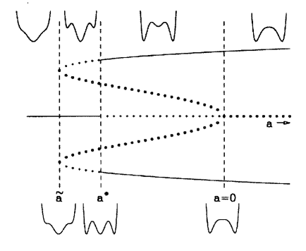
Figure 3.1: Bifurcation diagram for the subcritical bifurcation showing stationary solutions of $x$ vs. the control parameter $a$. The form of the potential $V$ for different values of $a$ is also shown. Solid lines denote stable states. Dots and crosses stand, respectively, for unstable and metastable states, where $\tilde{a}=-{b^{2}\over 4c}$, $a^{*}=-{3b^{2}\over 16c}$.

We are here interested in describing the relaxation triggered by noise from the state $x=0$. In a supercritical bifurcation $b<0$ and we consider the relaxation for $a>0$. In this case the quintic term in (3.1) is irrelevant and we can set $c=0$. In a subcritical bifurcation $b>0$. When $-{3b^{2}\over 16c}<a<0$, $x=0$ is a metastable state and it becomes unstable for $a>0$. Changing the control parameter $a$ from negative to positive values there is a crossover in the relaxation mechanism from relaxation via activation to relaxation from an unstable state. The bifurcation diagram for the subcritical bifurcation is shown in Fig. (3.1). We will first consider the relaxation from $x=0$ in the supercritical case ($a>0$,$b<0$, $c=0$) and secondly the relaxation in the critical case $a=0$ of the subcritical bifurcation ($b>0$, $c<0$). In the supercritical case the state $x=0$ is an unstable state and the relaxation process follows, initially, Gaussian statistics for $x$. However, the state $x=0$ has marginal stability in the case of a subcritical bifurcation for relaxation with $a=0$, and in this case Gaussian statistics, or equivalently, linear theory, does not hold at any time of the dynamical evolution.

A usual approach to the statistical description of (3.1) features the Fokker Planck equation (see Sect. 2.3) for the probability density $P(x,t)$ of the process, (see Fig. (3.2))

$$\partial_{t}P(x,t)=\partial_{x}(\partial_{x}V)P+\epsilon\partial^{2}_{x}P\equiv HP(x,t),$$ (3.3)

where $H$ is the Fokker-Planck operator. Equations for the time dependent moments of the process $x(t)$ are easily obtained from (3.3). The calculation of PT statistics is also standard [1, 2, 52] for a Markov process $x(t)$: the probability that at time $t$, $x(t)$ is still in an interval $(x_{1},x_{2})$ given an initial condition $x_{0}$ at $t=0$ is known as the survival probability $F({x_{0}},t)$. It obeys the equation

$$\partial_{t}F({x_{0}},t)=H^{+}_{D}F({x_{0}},t)$$ (3.4)

where $H_{D}^{+}$ is the adjoint of $H_{D}$. The latter operator differs from $H$ in that it avoids the probability of reentering the interval $(x_{1},x_{2})$ after having left it. The FPTD is given by $f({x_{0}},t)=-\partial_{t}F({x_{0}},t)$, and as a consequence the MFPT, $T_{x_{0}}$, obeys the Dynkin equation

$$H_{D}^{+}T_{x_{0}}=-1.$$ (3.5)

The lifetime $T$ of the state $x=0$ is given by the MFPT for $x^{2}$ to reach a value $R_{0}^{2}$ starting at $x=0$. From (3.5) we obtain

$$T={2\over\epsilon}\int_{0}^{R_{0}}dx{{}_{1}}e^{V(x{{}_{1}})/\epsilon}\int_{0}^{x_{1}}e^{V(x{{}_{2}})/\epsilon}dx_{2}.$$ (3.6)

Figure 3.2: Schematic evolution of the probability density $P(x,t)$ for the decay from $x=0$ in a supercritical bifurcation: An initial distribution centered in $x=0$ broadens and develops two peaks around the deterministic steady state solutions $x=\pm(-a/b)^{1/2}$. Time evolution is (a) $\rightarrow$ (b) $\rightarrow$ (c) $\rightarrow$ (d).

This relation is generally valid. In the supercritical case, and for asymptotically small $\epsilon$, we obtain

$$T\sim{1\over 2a}\ln{aR^{2}_{0}\over\epsilon}-{\psi(1)\over 2a}\sim{1\over 2a}\ln\epsilon^{-1},$$ (3.7)

where $\psi$ is the digamma function [19]. The variance of the FPT distribution is given by

$$(\Delta T)^{2}={1\over 4a^{2}}\psi^{\prime}(1).$$ (3.8)

We note that while in a deterministic treatment, $x(t)$ starts to grow exponentially as $x^{2}\sim e^{2at}$, the lifetime of the state is not simply $a^{-1}$ because such lifetime is determined by fluctuations and it diverges logarithmically with $\epsilon$. On the other hand, $(\Delta T)^{2}$ turns out to be independent of $\epsilon$ in the limit of small noise intensity. The same type of calculation for the subcritical bifurcation [53, 54] gives a formula for $T$ which interpolates between the Kramers result for relaxation from a metastable state, obtained for $a<0$ and $|k|\gg 1$, and (3.7) for relaxation from an unstable state, obtained for $a>0$ and $|k|\gg 1$. The parameter $k\equiv a/(b\epsilon)^{1/2}$ measures the distance to the situation of marginality $a=0$.

As we stressed in the previous section much physical insight can be gained following the actual stochastic trajectories $x(t)$ (Fig. (3.3)). We will now use this approach to describe the relaxation process and to reobtain the results quoted above for the distribution of passage times. A first intuitive idea of an individual trajectory in the supercritical case distinguishes two dynamical regimes in the relaxation process: There is first a linear regime of evolution in which the solution of (3.1) can be written ($b=c=0$) as

$$x(t)=h(t)e^{at},\quad h(t)=\sqrt{\epsilon}\int^{t}_{0}dt^{\prime}e^{-at^{\prime}}\xi(t^{\prime}),$$ (3.9)

where $h(t)$ is a Gaussian process which plays the role of a stochastic time dependent initial condition which is exponentially amplified by the deterministic motion. There is a second time regime in which noise along the path is not important, and the trajectory follows nonlinear deterministic dynamics from a nonzero initial condition $x(0)$. The deterministic solution of (3.1) ($\epsilon=0$) is

$$x(t)={x(0)e^{at}\over[1-{b\over a}x^{2}(0)(e^{2at}-1)]^{1/2}}.$$ (3.10)

Figure 3.3: A sample of individual trajectories for the decay process obtained from a numerical solution of (3.1) with $x(0)=0$, $a=1$, $b=-1$, $c=0,\epsilon=10^{-8}$., and different realizations of the noise. The vertical bars indicate the difference between the most separated trajectories at a fixed time. The evolution of an average trajectory $\langle x^{2}(t)\rangle$ and a statistical spread $\delta(t)=\langle x^{2}(t)\rangle-\langle|x(t)|\rangle^{2}$ is also shown. The form of $\delta(t)$ is associated with transient anomalous fluctuations.

A theory for the relaxation process is based on this separation of dynamical regimes observed in each trajectory. In this theory the complete stochastic evolution is replaced by the nonlinear deterministic mapping of the initial Gaussian process $h(t)$: The stochastic trajectory is approximated by replacing the initial condition $x(0)$ in (3.10) by $h(t)$ so that $x(t)$, becomes the following functional of the process $h(t)$:

$$x([h(t)],t)={h(t)e^{at}\over[1-{b\over a}h^{2}(t)(e^{2at}-1)]^{1/2}}.$$ (3.11)

Eq. (3.11) implies a dynamical scaling result for the process $x(t)$, in the sense that $x(t)$ is given by a time dependent nonlinear transformation of another stochastic process, namely the Gaussian process $h(t)$. This result for $x(t)$ is also often called the quasideterministic theory (QDT) [55] and has alternative presentations and extensions [45, 56]. The fact that Eq. (3.11) gives an accurate representation of the individual trajectories of (3.1) (except for the small fluctuations around the final steady state $x{{}_{f}^{2}}=-a/b$) justifies the approach.

In the approximation (3.11) the PT are calculated as random times to reach a given value $R_{0}$ within the linear stochastic regime. In fact, $T$ sets the upper limit of validity of the linear approximation. The process $h(t)$ has a second moment $\langle h^{2}(t)\rangle={\epsilon\over a}(1-e^{-2at})$ which saturates to a time independent value far from criticality, $at\gg 1$. In this limit the process $h(t)$ can be replaced by a Gaussian random variable $h(\infty)$ with $\langle h(\infty)\rangle=0$ and $\langle h^{2}(\infty)\rangle={\epsilon\over a}$. This permits to solve (3.9) for the time $t^{*}$ at which $R_{0}$ is reached

$$t^{*}={1\over 2a}\ln{R^{2}_{0}\over h^{2}(\infty)}.$$ (3.12)

This result gives the PT statistics as a transformation of the random variable $h=h(\infty)$. The statistical properties are, for example, completely determined by the generating function

$$W(\lambda)=\langle e^{-\lambda t^{*}}\rangle=\int dhP(h)e^{-\lambda t^{*}(h)},$$ (3.13)

where $P(h)$ is the known Gaussian probability distribution of $h(\infty)$. Moments of the PT distribution are calculated by differentiation with respect to $\lambda$ at $\lambda=0$. In this way one recovers (3.7) and (3.8). We note that this calculation assumes a separation of time scales between $a^{-1}$ and $T$. When this separation fails there is no regime of linear evolution. The decay process is then dominated by fluctuations and nonlinearities (see an example in Sect. 5.2).

Time dependent moments of $x(t)$ can also be calculated from the approximated trajectory (3.11) by averaging over the Gaussian probability distribution $P(h,t)$ of the process $h(t)$:

$$\langle x^{n}(t)\rangle=\int dhP(h,t)x^{n}([h(t)],t)$$ (3.14)

It turns out that in the limit $e^{at}\gg 1$ there is dynamical scaling in the sense that the moments only depend on time through their dependence in the parameter $\tau={\epsilon\over a}e^{2at}$. The result for $\langle x^{n}(t)\rangle$, given in terms of hypergeometric functions, can then be expanded in a power series in $\tau$ [45]. For example for the second order moment one obtains:

$$\langle x^{2}(t)\rangle=\langle x^{2}({\infty})\rangle\sum^{\infty}_{n=1}(-1)^{n-1}(2n-1)!!\tau^{n}.$$ (3.15)

This result indicates that our approximation to the trajectory corresponds to a summation of the perturbative series in the noise intensity $\epsilon$ which diverges term by term with time. It also gives an interpretation of the MFPT as the time $t$ for which the scaling parameter $\tau\sim 1$. For times of the order of the MFPT the amplification of initial fluctuations gives rise to transient anomalous fluctuations of order $\epsilon^{0}$ as compared with the initial or final fluctuations of order $\epsilon$ as shown in Fig. (3.3): At early and late times of the decay process different trajectories are close to each other at a fixed time, resulting in a small dispersion as measured by $\delta(t)$. However, at intermediate times the trajectories are largely separated as a consequence of the amplification of initial fluctuations and $\delta(t)$ shows a characteristic peak associated with large transient fluctuations.

The scaling theory discussed above can be put in a more systematic basis which can also be used in the subcritical case: In order to approximate the individual paths of the relaxation process defined by (3.1) and $x(0)=0$, we write $x(t)$ as the ratio of two stochastic processes

$$x(t)=z(t)/y^{1/2}(t)$$ (3.16)

Then (3.1) (with $c=0$) is equivalent to the set of equations

$$d_{t}z(t)=az(t)+\sqrt{\epsilon}y^{1/2}(t)\xi(t)$$ (3.17)

$$d_{t}y(t)=-2bz^{2}(t),$$ (3.18)

with $z(0)=x(0)=0$, $y(0)=1$. Eqs. (3.17)-(3.18) can be solved iteratively from the initial conditions. In the zero–th order iteration

$$x(t){\sim}z(t)=h(t)e^{at},$$ (3.19)

where

$$h(t)=\sqrt{\epsilon}\int^{t}_{0}e^{-as}\xi(s)ds,$$ (3.20)

is a Gaussian stochastic process. In the first order iteration

$$x(t)={e^{at}h(t)\over[1-2b\int_{0}^{t}e^{2as}h^{2}(s)ds]^{1/2}}.$$ (3.21)

In this approximation the decomposition (3.16) is interpreted as follows. The process $z(t)$ coincides with the linear approximation ($b=0$,$c=0$) to (3.1). The process $y(t)$ introduces saturation effects killing the exponential growth of $z(t)$. The scaling theory approximation (3.11) is recovered from this approach whenever $at\gg 1$ so that

$$\int_{0}^{t}e^{2as}h^{2}(s)ds\sim{1\over{2a}}h^{2}(t)(e^{2at}-1)$$ (3.22)

This indicates that the regime in which the scaling theory is valid is rapidly achieved far from the condition of criticality $a\sim 0$.

We next consider the relaxation from $x=0$ with $a=0$ in a subcritical bifurcation $b>0$ [57]. As we did before we look for a decomposition of the form (3.16). Since we are only interested in the escape process we set $c=0$ in (3.1). Eq. (3.1) with $a=c=0$ is equivalent to the set (3.17)-(3.18) with $a=0$. In the zero–th order iteration

$$x(t)\sim z(t)=\sqrt{\epsilon}W(t),\quad W(t)=\int_{0}^{t}\xi(s)ds.$$ (3.23)

The process $x(t)$ coincides with the Wiener process giving diffusion in the locally flat potential $V$. In the first order iteration we find

$$x(t)={{\sqrt{\epsilon}W(t)}\over{[1-2\epsilon b\int_{0}^{t}W^{2}(s)ds]^{1/2}}}.$$ (3.24)

Two important differences between (3.24) and (3.21) should be stressed. The first one is that in the first stage of evolution given by (3.23) there is no escape from $x=0$. The nonlinearities introduced by the process $y(t)$ are essential for the escape process to occur. This means that, contrary to the case of (3.21), there is no regime of the escape process in which Gaussian statistics holds. The second difference is that $x(t)$ given by (3.24) does not have a scaling form, since it is not a transformation of a single stochastic process. Indeed, $x(t)$ in (3.24) depends on two non independent processes, namely $W(t)$ and $\int_{0}^{t}W^{2}(s)ds$. A naive approach to the problem would be to assume, by analogy with (3.11), a scaling form in which $x(t)$ is given by the deterministic nonlinear mapping of the fluctuating initial process $\sqrt{\epsilon}W(t)$, i.e., $x(t)$ given by the deterministic solution of (3.1) with $x(0)$ replaced by $\sqrt{\epsilon}W(t)$. This would amount to take $y(t)=1-2\epsilon btW^{2}(t)$. This scaling representation is qualitatively incorrect since it leads to a diverging MPT, $T=\infty$. The accuracy of the representation (3.24) is shown in Fig. (3.4) where an individual trajectory given by (3.24) is compared with the corresponding one of the exact process given by (3.1). In this figure we observe that $x(t)$ coincides initially with the Wiener process, it later departs from it and at a time rather sharply defined it departs from the vicinity of $x=0$. In fact, the strong nonlinearity implies that the solution of (3.1) with $c=0$ and $x(0)\neq 0$ reaches $|x|=\infty$ in a finite time. It is then natural to identify the PT for the escape from $x=0$ as a random time $t^{*}$ for which $|x(t^{*})|=\infty$ in (3.24), or equivalently $y(t^{*})=0$. From (3.24) we find

$$1=2b\epsilon\int_{0}^{t^{*}}W^{2}(s)ds.$$ (3.25)

Taking into account that $W^{2}(t^{*}s)=t^{*}W^{2}(s)$, (3.25) can be solved for $t^{*}$ as

$$t^{*}=\left[1\over{2b\epsilon\Omega}\right]^{1/2},$$ (3.26)

with

$$\Omega\equiv\int_{0}^{1}W^{2}(s)ds.$$ (3.27)

Eq. (3.26) gives the statistics of $t^{*}$ as a transformation of the statistics of another random variable $\Omega$. This scaling result for $t^{*}$ has the same basic contents than (3.12). In (3.12) the result appeared for $at\gg 1$ as a consequence of Gaussian statistics while here the transformation (3.26) appears as an exceptional scaling at the critical point $a=0$, and $\Omega$ has non-Gaussian statistics. A discussion of the crossover between these two regimes is given in [53].

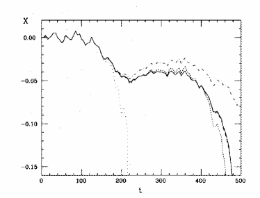
Figure 3.4: Stochastic paths in the decay from $x=0$ for $a=0$ in the subcritical bifurcation with $b=c=1$ and $\epsilon=10^{-6}$. Different paths correspond to different approximations for the same realization of the noise. The solid line corresponds to a simulation of the exact process given by (3.1). Dotdashed line corresponds to a Wiener process. Dots correspond to the scaling approach similar to (3.11) (see text) and the dashed line corresponds to the approximation (3.24).

The calculation of the statistics of $t^{*}$ from (3.26) requires the knowledge of the statistics of $\Omega$. The latter is completely determined by the generating function $G(\lambda)$, for which an exact result is available [57],

$$G(\lambda)\equiv\langle e^{-\lambda\Omega}\rangle=(\cosh(2\lambda^{1/2}))^{-1/2}.$$ (3.28)

The moments of the PTD are obtained from (3.26) in terms of $G(\lambda)$ as

$$\langle t^{*2n}\rangle={{(2b\epsilon)^{-n}}\over{\Gamma(n)}}\int_{0}^{\infty}d\lambda\quad\lambda^{n-1}G(\lambda).$$ (3.29)

The transient moments $\langle x^{n}(t)\rangle$ can also be obtained in terms of the statistics of the PT [57]: Given the strong nonlinearity of the escape process a good approximation to calculate ensemble averages is to represent $x(t)$ by

$$x^{2}(t)=x^{2}(\infty)\theta(t-t^{*}),$$ (3.30)

where $x(\infty)$ is the final stable state (local minima of the potential V) and $\theta(t-t^{*})$ is the Heaviside step function. The individual path is approximated by a jump from $x=0$ to $x=x(\infty)$ at a random time $t^{*}$. The transient moments are then easily calculated as averages over the distribution of the times $t^{*}$.

The methodology described here to characterize relaxation processes by focusing on the statistics of the passage times can be generalized to a variety of different situations which include colored noise [58], time dependent control parameter $a(t)$ sweeping through the instability at a finite rate [59, 60], competition between noise driven decay and decay induced by a weak external signal [61], role of multiplicative noise in transient fluctuations [62], saddle-node bifurcation [63], etc. We have limited here ourselves to transient dynamics in stochastic processes defined by a SDE of the Langevin type, but the PT characterization is also useful, for example, in the framework of Master Equations describing transport in disordered systems [54, 64]

3.2 Statistics of laser switch-on

Among the applications to different physical systems of the method described above, the analysis of the stochastic events in the switch-on of a laser is particularly interesting for several reasons. Historically (see the review in [47]) the concept of transient anomalous fluctuations already appeared in this context in the late 60’s, and from there on a detailed experimental characterization exists for different cases and situations. The idea of noise amplification is also very clear here, and for example the term ”statistical microscope” [65] has been used to describe the idea of probing the initial spontaneous emission noise through the switch-on amplification process. From the methodological point of view the idea of following the individual stochastic trajectory has in this context a clear physical reality. While in more traditional equilibrium statistical physics it is often argued that measurements correspond to ensemble averages, every laser switch-on is an experimental measured event which corresponds to an individual stochastic trajectory. Also here the PT description has been widely used experimentally [66]. Finally, from an applied point of view, the variance of the PT distribution for the switch-on of a semiconductor laser sets limitations in the maximum transmission rate in high speed optical communication systems [67, 68]. We will limit our quantitative discussion here to semiconductor lasers. A review of other situations is given in [48].

The dynamics of a single mode semiconductor laser can be described by the following equations for the slowly varying complex amplitude of the electric field $E$ and the carrier number $N$ [67, 69, 70, 71, 72]:

$$\partial_{t}E={1+i\alpha\over 2}[G-\gamma]E+\sqrt{\beta N}\xi_{E}(t),$$ (3.31)

$$\partial_{t}N=C-\gamma_{e}N-G|E|^{2}-\sqrt{4\beta N}[E^{*}\xi_{E}(t)+E\xi_{E}^{*}(t)].$$ (3.32)

Terms proportional to the gain coefficient $G$ account for stimulated emission and, to a first approximation, $G=g(N-N_{0})$, where $g$ is a gain parameter and $N_{0}$ the value of carrier number at transparency. The control parameter of the system is here the injection current $C$. Spontaneous emission is modeled by a complex Gaussian white noise $\xi_{E}(t)$ of zero mean and correlation

$$\langle\xi_{E}(t)\xi_{E}^{*}(t^{\prime})\rangle=2\delta(t-t^{\prime}).$$ (3.33)

Noise is here multiplicative and its intensity is measured by the spontaneous emission rate $\beta$. The noise term in the equation for $N$ can be usually neglected . The variables $E$ and $N$ have decay rates $\gamma$ and $\gamma_{e}$ such that $\gamma\sim 10^{3}\gamma_{e}$. This implies that the slow variable is $N$, and that when the laser is switched-on the approach to the final state is not monotonous. Rather, a light pulse is emitted followed by damped oscillations called relaxation oscillations. This also occurs for $CO_{2}$ and solid state lasers, but there are other lasers such as He-Ne (“class Alasers”) in which $E$ is the slow variable, the approach is monotonous and a simpler description with a single equation for $E$ holds. Such description is similar to the one in Sect. 3.1 [48]. Finally, the $\alpha$-parameter, or linewidth enhancement factor, gives the coupling of phase $\phi$ and laser intensity $I$ ($E=I^{1/2}e^{i\phi}$).

$$\partial_{t}I=(G-\gamma)I+4\beta N+\sqrt{4\beta NI}\xi_{I}(t),$$ (3.34)

$$\partial_{t}\phi={\alpha\over 2}(G-\gamma)+\sqrt{4\beta N\over I}\xi_{\phi}(t),$$ (3.35)

where $\xi_{I}$ and $\xi_{\phi}$ are the intensity and phase noise components of $\xi_{E}$. These equations are conventionally written as Itô SDE. The instantaneous frequency of the laser is the time derivative of the phase. Transient frequency fluctuations for class A lasers were discussed in [73].

To switch-on the laser, the injection current $C$ is switched, at a time $t=0$, from below to above its threshold value $C_{th}=({\gamma\over g}+N_{o})\gamma_{e}$. Below threshold the laser is off with $I$ fluctuating around $I=0$. The steady state value above threshold is given by $I={1\over\gamma}(C-C_{th})+0(\beta)$ and $N=N_{th}={C_{th}\over\gamma_{e}}$. An example of the early time dynamics in the approach to this steady state is shown in Fig. (3.5) where two switch-on events corresponding to two different stochastic trajectories are shown. We observe that the laser switches-on when $N$ reaches a maximum value. This happens at a random time which gives the delay from the time at which $C$ is switched. The dispersion in the delay times is known as “jitter”. We will characterize the switch-on statistics by the PT distribution for $I$ to reach a given reference value. We also observe a statistical spread in the height $I_{M}$ of the light pulses (maximum output power) for different switch-on events, being larger for longer delay times. The frequency of the laser shows huge fluctuations while it is off, and it drifts from a maximum to a minimum frequency during the emission of the light pulse due to the phase-amplitude coupling caused by the $\alpha$-parameter. This excursion in frequency is known as “frequency chirp”, and again there is a statistical distribution of chirp for different switch-on events. Relevant questions here are the calculation of switch-on times, maximum laser intensity and chirp statistics, as well as the relation among them.

The calculation of switch-on time statistics follows the same basic ideas than in Sect. 3.1 [70, 72]: We consider the early linearized regime formally obtained setting $G=0$ in the equation for $N$. When the solution of this equation is substituted in (3.31) we still have a linear equation for $E$ but with time dependent coefficients, so that,

$$E(t)=e^{A(t)/2}h(t),$$ (3.36)

$$A(t)=(1+i\alpha)\int^{t}_{\bar{t}}dt^{\prime}[g(N(t^{\prime})-N_{o})-\gamma],$$ (3.37)

$$h(t)=\int^{t}_{\bar{t}}dt^{\prime}\sqrt{\beta N(t^{\prime})}\xi(t^{\prime})e^{-A(t^{\prime})/2},$$ (3.38)

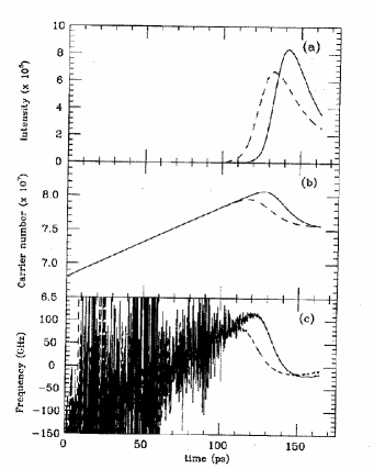
Figure 3.5: Time evolution of (a) laser intensity $I=|E|^{2}$, (b) carrier number $N$ and (c) frequency $f=(2\pi)^{-1}{\Delta\phi\over\Delta t}$ as obtained from the numerical integration of Eqs. (3.31)-(3.32) for typical parameter values and for two different switch-on transients: solid and dashed line. Times are given in picoseconds.

where we have chosen a reference time ${\bar{t}}$, $N(\bar{t})=N_{th}$. We note that for ordinary parameter values $N(t)$ grows linearly with $t$ around ${\bar{t}}$ (as it is seen in Fig. (3.5)), so that $A(t)\sim(t-\bar{t})^{2}$. The important fact is again that the complex Gaussian process $h(t)$ saturates for times of interest to a complex Gaussian random variable $h(\infty)$ of known statistics. We can then solve (3.36) for the time $t^{*}$ at which the reference value $I_{r}=|E_{r}|^{2}$ of $I$ is reached

$$(t^{*}-\bar{t})^{2}\sim\ln{I_{r}\over|h(\infty)|^{2}}.$$ (3.39)

The statistics of $t^{*}$ are now easily calculated as a transformation of that of $h(\infty)$. In particular we obtain $(\Delta T)\ll T$, with

$$T=\langle t^{*}\rangle=\bar{t}+\sqrt{{2\tau\over g(C-C_{th})}}[1-{\psi(1)\over 2\tau}],\quad\tau=\ln{I_{r}\over b}$$ (3.40)

$$(\Delta T)^{2}={\psi^{\prime}(1)\over 2\tau g(C-C_{th})}$$ (3.41)

where $b$ is proportional to $\beta$.

We next address the calculation of the statistics of the maximum laser intensity $I_{M}$ [70, 74]. Fig (3.6) shows a superposition of different switch-on events, obtained from a numerical integration of (3.31)-(3.32), in which the statistical dispersion in the values of $I_{M}$ is evidentiated. The laser intensity peak value is reached well in the nonlinear regime and we adopt, as in Sect 3.1, the strategy of mapping the initial stochastic linear regime with the nonlinear deterministic dynamics. For each switch-on event, the deterministic equations should be solved with initial conditions at the time $t^{*}$ which identifies the upper limit of the linear regime: $E=E(t^{*})=E_{r}$ and $N=N(t^{*})$. The value of $N(t^{*})$ is calculated linearly and takes random values for different switch-on events. Eliminating the parameter $t$ the solution can be written in an implicit form as

$$E=E(N,E_{r},N(t^{*})).$$ (3.42)

Figure 3.6: Superposition of 50 switch-on events (50 individual stochastic trajectories) for the laser intensity as obtained from the numerical integration of Eqs.(3.31)-(3.32). The laser power $P$ is proportional to the laser intensity I.

Any arbitrary function $Y$ of the dynamic variables in which one might be interested can then be written as

$$Y(t)=Y(N(t),E(t))=Y(t,N(t^{*}),E_{r})=Y(N,E_{r},N(t^{*})).$$ (3.43)

To proceed further one generally needs an explicit form for the solution of the equations. However, important results can be already obtained if one is interested in extreme values of $Y$. The variable $Y$ takes an extreme value $Y_{e}$ at a time $t_{e}$ such that $\partial_{t}Y(t)=0$. This gives an additional implicit relation $N(t_{e})=N_{e}(E_{r},N(t^{*}))$ so that,

$$Y(t_{e})=Y_{e}(E_{r},N(t^{*})).$$ (3.44)

This equation gives the desired mapping of the statistical properties of the switch-on times $t^{*}$ into those of an extreme value of a dynamical variable: For each switch-on event there is a value of $t^{*}$ and a corresponding value $Y_{e}(t^{*})$. Taking advantage of the fact that $(\Delta T)\ll T$ we can expand $Y_{e}(t^{*})$ around $t^{*}=T$:

$$Y_{e}(t^{*})=Y_{e}(T)+{\partial Y_{e}\over\partial N(t^{*})}{\left.{dN\over dt^{*}}\right|}_{T}(t^{*}-T)+0(\Delta T)^{2}.$$ (3.45)

Applying this relation to the maximum output power, $Y_{e}=I_{M}$, it predicts a straight line for a plot of the values of $I_{M}$ vs. switch-on times obtained from many independent switch-on experiments. Such linear dependence can be already seen in Fig. (3.6). This prediction has been corroborated experimentally for $CO_{2}$ [74, 76], semiconductor [75] and solid state lasers [74]. The slope of this linear relation can be estimated in different cases. For semiconductor lasers [70] it is easily seen from the equations above, that the slope is positive and proportional to the distance to threshold $C-C_{th}$. However in other cases there is a predominant contribution of the initial fluctuations of $N(t=0)$ and the slope becomes negative [74].

Turning now to transient frequency fluctuations, a first delicate issue is the proper definition of an instantaneous frequency, since $\partial_{t}\phi$ in (3.35) contains a white noise noise contribution, and therefore, in principle, an infinite variance. A meaningful operational definition of the instantaneous frequency can be given in terms of a short time interval average of $\partial_{t}\phi$, or equivalently in terms of a time resolved field Fourier spectrum [71, 77]. From (3.35) we also see that there are two sources of frequency fluctuations. One is the noise along the path given by the phase noise $\xi_{\phi}$, and the second is the stochastic nature of the gain term $G$ for different switch-on events, due to the random nature of $t^{*}$. The first dominates steady state properties such as laser linewidth, but the second dominates transient properties such as the fluctuations in the chirp range. Since the chirp range is defined by a difference between two extreme values of the frequency the general framework discussed above applies. In fact one finds that the maximum and minimum instantaneous frequencies during the transient are linear functions of the switch-on time $t^{*}$ [72]. Chirp noise statistics is again calculated by a simple transformation of the switch-on time statistics.

We finally mention that the operation of a semiconductor laser in a system of optical communications involves a repetition of switch-on events (large signal modulation) to transmit pulses at a given bit-rate. Communication errors are likely to happen when $\Delta T$ is large or when memory effects are present. The effect of memory occurs when a given switch-on event is not independent of the previous one in very fast modulation. The determination of ”memory-free” regions in parameter space for a given modulation rate involves, as a crucial time scale of the problem, the mean switch-on time $T$ [78]. Other errors are due to pulse dispersion in the optical fibre because of large chirp noise [79].

4 Noise in Dynamical Systems

4.1 Classification of Dynamical Systems: Potentials and Lyapunov Functions

In this section, we will study the effect of noise in the long time behavior of dynamical systems. First of all, though, we will briefly review the basic concepts about the stability of dynamical systems [80].

Let $x\equiv(x_{1},\dots,x_{N})$ be a set of real dynamical variables. They follow the evolution equations:

$$\frac{dx_{i}}{dt}=f_{i}(x_{1},\dots,x_{N}),~{}~{}~{}~{}~{}~{}i=1,\dots,N$$ (4.1)

One is usually interested in finding the fixed points $\bar{x}$ of the dynamical system as those points which do not evolve in time, i.e. those satisfying:

$$\left.\frac{dx_{i}}{dt}\right|_{x=\bar{x}}=0,~{}~{}~{}~{}~{}~{}i=1,\dots,N$$ (4.2)

or, equivalently,

$$f_{i}(\bar{x}_{1},\dots,\bar{x}_{N})=0,~{}~{}~{}~{}~{}~{}i=1,\dots,N$$ (4.3)

Knowing the fixed points is as important as knowing their stability. Loosely speaking, a fixed point $\bar{x}$ is stable if any initial condition $x(0)$ sufficiently close to $\bar{x}$ remains close to $\bar{x}$ as time evolves. The fixed point is said to be asymptotically stable if any initial condition $x(0)$ sufficiently close to $\bar{x}$ tends to $\bar{x}$ as time evolves. Fig. (4.1) illustrates the concepts of stability and asymptotic stability.

Figure 4.1: Illustration of the concepts of stable and asymptotically stable fixed points.

To determine the stability of a fixed point, Lyapunov’s stability theorem is of great help. The theorem states that if we can find a Lyapunov function, $L(x)=L(x_{1},\dots,x_{N})$ which is such that it has a local minimum at $x=\bar{x}$ and monotonically decreases with time, i.e.:

$$\begin{array}[]{lll}(a)&L(x)>L(\bar{x})&{\rm for~{}}x\neq\bar{x}\\ (b)&{\displaystyle\frac{dL}{dt}=\sum_{i=1}^{N}\frac{\partial L}{\partial x_{i}}\frac{dx_{i}}{dt}\leq 0}&{\rm for~{}}x\neq\bar{x}\end{array}$$ (4.4)

then $\bar{x}$ is a stable fixed point. If condition (b) is replaced by

$$(b^{\prime})\hskip 2.84544pt\frac{dL}{dt}<0\hskip 28.45274pt{\rm for~{}}x\neq\bar{x}$$ (4.5)

then $\bar{x}$ is an asymptotically stable fixed point. $L(x)$ is also called a Lyapunov potential or, simply, the potential.

The description of the behaviour of a dynamical system is greatly simplified if we know of the existence of a Lyapunov potential: the system evolves towards the minima of the Lyapunov and once there it stays nearby when small perturbations act upon the system. The Lyapunov potential not only tells us about local stability, but also gives information about global stability. If two fixed points $\bar{x}^{(1)}$ and $\bar{x}^{(2)}$ are such that $L(\bar{x}^{(2)})<L(\bar{x}^{(1)})$ then we can infer that $\bar{x}^{(2)}$ is the stable fixed point and that $\bar{x}^{(1)}$ is a metastable fixed point. This means that a sufficiently strong perturbation might take the system out of $\bar{x}^{(1)}$ to $\bar{x}^{(2)}$. Therefore, to understand the asymptotic dynamics it is of great importance to find out whether a Lyapunov potential can be found for the dynamical system under study. It is not an easy task to (i) prove that the Lyapunov potential does exist, (ii) find it. The systems for which a Lyapunov function exists are called in the literature potential systems and the name non–potential systems is therefore reserved for those systems which do not have a Lyapunov function (notice that this is different from the fact that there is no known Lyapunov potential). According to these definitions, and following the ideas of Graham on nonequilibrium potential [81, 82, 83, 84], the following classification of dynamical systems can be established [85, 86]:
1.- Relaxational Gradient Flow
2.- Relaxational Non–Gradient Flow
3.- Non–Relaxational Potential Flow
4.- Non–Potential Flow
The first three categories are called potential flows. We now describe each of them in some detail.

(1) Relaxational Gradient Flow.
Those are systems for which there exists a function (the “potential”) $V(x)=V(x_{1},\dots,x_{N})$ in terms of which the dynamics is written as:

$$\frac{dx_{i}}{dt}=-\frac{\partial V}{\partial x_{i}}$$ (4.6)

The fixed points of this dynamical system are the extrema of the potential $V(x)$. The trajectories lead to any of the minimum values of $V(x)$ following the lines of maximum slope (steepest descent) as indicated schematically in Fig. (4.2).

Figure 4.2: Schematic trajectories for the case of relaxational gradient flow in two cases: a Lyapunov function with a single minimum (left picture) and a Lyapunov function with two minima (right picture). The system evolves towards one of the two minima, according to initial conditions, following the lines of maximum slope.

In this case the potential $V$ is a Lyapunov function. The proof of this statement is very simple indeed (we need the additional condition that $V(x)$ is bounded from below):

$$\frac{dV}{dt}=\sum_{i=1}^{N}\frac{\partial V}{\partial x_{i}}\frac{dx_{i}}{dt}=-\sum_{i=1}^{N}\left(\frac{\partial V}{\partial x_{i}}\right)^{2}\leq 0$$ (4.7)

An example of this class of systems is the real Ginzburg–Landau equation (see later), also known in the theory of critical dynamics as model $A$ in the classification of [87] (see Section 6).

(2) Relaxational non–Gradient Flow.
There exists again a potential function, $V(x)$, but now the dynamics is not governed just by $V$, but it is given by:

$$\frac{dx_{i}}{dt}=-\sum_{j=1}^{N}S_{ij}\frac{\partial V}{\partial x_{j}}$$ (4.8)

where $S_{ij}(x)$ is a real, symmetric, positive definite matrix. The fixed points of the dynamics are still given by the extrema of $V$ and the trajectories lead to the minima of $V$ but not necessarily through the lines of maximum slope. In this sense, we can say that the transient dynamics is not governed just by the potential. Fig. (4.3) shows schematically the situation. A typical example of this dynamics is the so–called Cahn–Hilliard [88] model for spinodal decomposition [46] or model $B$ in the context of critical dynamics [87]. In this model the dynamical variables represent a concentration field that follows a conservation law:

$$\frac{d~{}}{dt}\sum_{i=1}^{N}x_{i}=0$$ (4.9)

This constrain is satisfied by choosing $S=-\nabla^{2}$, the lattice Laplacian as defined, for instance, in (2.134).

Figure 4.3: Schematic trajectories for the case of relaxational non–gradient flow. The system evolves towards the minimum of the potential, but not necessarily through the lines of maximum slope.

In this case, the potential $V$ is still a Lyapunov functional:

$$\frac{dV}{dt}=\sum_{i=1}^{N}\frac{\partial V}{\partial x_{i}}\frac{dx_{i}}{dt}=-\sum_{i,j=1}^{N}S_{ij}\frac{\partial V}{\partial x_{i}}\frac{\partial V}{\partial x_{j}}\leq 0$$ (4.10)

since, by definition, $S$ is a positive definite matrix.

(3) Non–Relaxational Potential flow.
These systems are characterized because the asymptotic behavior is not determined simply by the minima of the potential, but there is a residual dynamics once those minima have been reached. A first category within this class is given by:

$$\frac{dx_{i}}{dt}=-\sum_{j=1}^{N}D_{ij}\frac{\partial V}{\partial x_{j}}$$ (4.11)

Here, $D_{ij}(x)$ is an arbitrary matrix that can be split into symmetric and antisymmetric parts:

$$D=S+A\left\{\begin{array}[]{rcl}S&=&\frac{1}{2}(D+D^{T})\\ A&=&\frac{1}{2}(D-D^{T})\end{array}\right.$$ (4.12)

and we demand that $S$ is positive definite matrix. Again, the fixed point of the dynamics are determined by the extrema of the potential $V$ and $V$ is a Lyapunov potential:

$$\frac{dV}{dt}=-\sum_{i,j=1}^{N}S_{ij}\frac{\partial V}{\partial x_{i}}\frac{\partial V}{\partial x_{j}}-\sum_{i,j=1}^{N}A_{ij}\frac{\partial V}{\partial x_{i}}\frac{\partial V}{\partial x_{j}}\leq 0$$ (4.13)

The second sum of this expression is zero due to the antisymmetry of matrix $A$. We are then led to the situation sketched in Fig. (4.4): the system evolves towards the minima of $V$ but once it reaches there, there is a residual movement produced by the antisymmetric part of the dynamical coefficients that can make the system flow without cost of the Lyapunov function.

Figure 4.4: Schematic trajectories for the case of non–relaxational potential flow. The system evolves towards the (degenerate) minima of the potential $V$ and, once it has reached there, there is a residual movement on an iso–potential region.

The dynamics of the nematodynamics equations commonly used to describe the dynamics of liquid crystals in the nematic phase belongs to this class, as shown in [89].

The second, more general, category of non–relaxational potential flow will be one in which the dynamical equations can be split into two parts, namely:

$$\frac{dx_{i}}{dt}=f_{i}\equiv-\sum_{j=1}^{N}S_{ij}\frac{\partial V}{\partial x_{j}}+v_{i}$$ (4.14)

Here $S(x)$ is a symmetric, positive definite matrix and $v_{i}(x)$ represents the residual dynamics after the relaxational part has acted. Since we want $V$ to be a Lyapunov potential the residual dynamics must not contribute to its decay:

$$\frac{dV}{dt}=-\sum_{i,j=1}^{N}S_{ij}\frac{\partial V}{\partial x_{i}}\frac{\partial V}{\partial x_{j}}+\sum_{i=1}^{N}v_{i}\frac{\partial V}{\partial x_{i}}\leq 0$$ (4.15)

or, since the first term of the r.h.s. is always negative, a sufficient condition is:

$$\sum_{i=1}^{N}v_{i}\frac{\partial V}{\partial x_{i}}=0$$ (4.16)

This is the so–called orthogonality condition. By using (4.14) can be written as:

$$\sum_{i=1}^{N}\left(f_{i}+\sum_{j=1}^{N}S_{ij}\frac{\partial V}{\partial x_{j}}\right)\frac{\partial V}{\partial x_{i}}=0$$ (4.17)

or, in compact vector notation:

$$(\vec{f}+S\vec{\nabla}V)\cdot\vec{\nabla}V=0$$ (4.18)

It can be shown that this equation has the structure of a Hamilton–Jacobi equation and in general it is very difficult to solve to find the potential $V$, although important results have been obtained in the literature [81, 83, 84].

(4) Non–Potential flow.
Finally, a non–potential flow is one for which the splitting (4.14), satisfying (4.15), admits only the trivial solution $V=0$, $v_{i}=f_{i}$. Notice that for a system to be classified as non–potential, we have to prove the non–existence of non–trivial solutions of (4.17) which, of course, it is not the same that not being able to find non–trivial solutions of (4.17).

Let us consider in detail an example of the previous classification scheme: the complex Ginzburg–Landau equation (CGLE) [86, 91, 92].

Let $A(\vec{r},t)$ be a complex field satisfying the equation of motion:

$$\frac{\partial A}{\partial t}=\mu A+\gamma\nabla^{2}A-\beta|A|^{2}A$$ (4.19)

$\mu=\mu_{R}+i\mu_{I}$, $\beta=\beta_{R}+i\beta_{I}$ and $\gamma=\gamma_{R}+i\gamma_{I}$ are complex numbers. This is the so–called complex Ginzburg–Landau equation [90]. It appears in a great variety of situations and it is a generic equation for the slow varying amplitude of the most unstable model near a Hopf bifurcation in an extended system (see Sect. 5.3). This might be put in what is called in the literature a “potential” form:

$$\frac{\partial A}{\partial t}=-\frac{\delta V}{\delta A^{*}}$$ (4.20)

where the “potential” $V$ is given by:

$$V\{A,A^{*}\}=\int d\vec{r}\left[-\mu|A|^{2}+\gamma|\vec{\nabla}A|^{2}+\frac{\beta}{2}|A|^{4}\right]$$ (4.21)

This, being of course true, is somewhat misleading because the function $V$ does not have most of the properties associated with a potential function as defined in the previous sections. In particular it can not be a Lyapunov function because it generally takes complex values.

We pose now the problem in a different form. Considering the evolution of the real and imaginary components of $A(\vec{r},t)=X(\vec{r},t)+iY(\vec{r},t)$, is it possible to find a real function $\tilde{V}(X,Y)$ such that the flow is relaxational gradient? i.e.

$$\left.\begin{array}[]{rcl}\displaystyle{\frac{\partial X}{\partial t}}&=&\displaystyle{-\frac{\delta\tilde{V}}{\delta X}}\\ \displaystyle{\frac{\partial Y}{\partial t}}&=&\displaystyle{-\frac{\delta\tilde{V}}{\delta Y}}\end{array}\right\}$$ (4.22)

This would imply:

$$\frac{\delta~{}}{\delta Y}\left(\frac{\partial X}{\partial t}\right)=\frac{\delta~{}}{\delta X}\left(\frac{\partial Y}{\partial t}\right)$$ (4.23)

which leads to

$$\mu=\mu^{*}\hskip 28.45274pt\gamma=\gamma^{*}\hskip 28.45274pt\beta=\beta^{*}$$ (4.24)

i.e. a complex Ginzburg–Landau equation with real coefficients.

In general, though, when the coefficients are complex there is no obvious Lyapunov function. However, there is an interesting case in which the dynamics can be put in the category (3) described above: there exists a split of the dynamics in terms of a potential term plus an extra term which, being orthogonal to the first, does not contribute to the variation of the Lyapunov potential. The easiest way of showing this is noticing that if we write $V(A,A^{*})=V_{R}(X,Y)+iV_{I}(X,Y)$ the variation of the real part is:

$$\begin{array}[]{rcl}\frac{dV_{R}}{dt}&=&-\frac{1}{2}\int d\vec{r}\left[\left(\frac{\delta V_{R}}{\delta X}\right)^{2}+\left(\frac{\delta V_{I}}{\delta Y}\right)^{2}\right]+\\ &&2(\gamma_{I}\beta_{R}-\beta_{I}\gamma_{R})\int d\vec{r}(X^{2}+Y^{2})\vec{\nabla}(Y\vec{\nabla}X-X\vec{\nabla}Y)\end{array}$$ (4.25)

It is clear now that if the following condition is fulfilled

$$\gamma_{I}\beta_{R}-\beta_{I}\gamma_{R}=0$$ (4.26)

$V_{R}$ acts as a Lyapunov. Introducing $\hat{V}=V/2$ the dynamical system can be written as:

$$\pmatrix{\frac{\partial X}{\partial t}\cr\frac{\partial X}{\partial t}}=-\pmatrix{\frac{\delta\hat{V}_{R}}{\delta X}\cr\frac{\delta\hat{V}_{R}}{\delta Y}}+\pmatrix{\frac{\delta\hat{V}_{I}}{\delta Y}\cr-\frac{\delta\hat{V}_{I}}{\delta X}}$$ (4.27)

and the orthogonality condition is:

$$\left(\frac{\delta\hat{V}_{I}}{\delta Y},-\frac{\delta\hat{V}_{I}}{\delta X}\right)\pmatrix{\frac{\delta\hat{V}_{R}}{\delta X}\cr\frac{\delta\hat{V}_{R}}{\delta Y}}=0$$ (4.28)

which is satisfied by condition (4.26). In this case a change of variables of the form $A(\vec{r},t)\rightarrow A(\vec{r},t){\rm e}^{i\alpha t}$ for a convenient value of $\alpha$ leads to

$$\frac{\partial A}{\partial t}=-(1+i)\frac{\delta V_{R}}{\delta A^{*}}$$ (4.29)

The $1$ in the r.h.s. is the real CGLE and the $i$ in the r.h.s. gives rise to a form of the Nonlinear Schrödinger equation.

We finally mention that although for general complex coefficients $\mu$, $\beta$ and $\gamma$ there is no simple form for a Lyapunov functional, this does not mean that there is no solution for the orthogonality condition (4.17). In fact, Graham and collaborators [91, 92] have found an approximate Lyapunov function for the CGLE by a gradient expansion solution of the orthogonality condition (4.17). A numerical test of its Lyapunov properties and a discussion of such Lyapunov function for the CGLE is given in [86].

4.2 Potentials and Stationary Distributions

We will see now which is the effect of noise on the dynamics of the above systems. To this end, we consider the general dynamics with the addition of a general noise term (to be considered in the Itô sense):

$$\dot{x}_{i}=f_{i}(x)+\sum_{j=1}^{N}g_{ij}\xi_{j}(t)$$ (4.30)

where $g_{ij}(x)$ are arbitrary functions and $\xi_{j}(t)$ are white noise variables: random Gaussian variables of zero mean and correlations:

$$\langle\xi_{i}(t)\xi_{j}(t^{\prime})\rangle=2\epsilon\delta_{ij}\delta(t-t^{\prime})$$ (4.31)

$\epsilon$ is the noise intensity, which is included here explicitly. Due to the presence of the noise terms, it is not adequate to talk about fixed points of the dynamics, but consider instead the maxima of the probability distribution function $P(x,t)$. This satisfies the multivariate Fokker–Planck equation [3]:

$$\frac{\partial P(x,t)}{\partial t}=\sum_{i=1}^{N}\frac{\partial~{}}{\partial x_{i}}\left[-f_{i}P+\epsilon\sum_{j=1}^{N}\frac{\partial~{}}{\partial x_{j}}\left(G_{ij}P\right)\right]$$ (4.32)

where the matrix $G$ is

$$G=g\cdot g^{T}$$ (4.33)

For the case of relaxational (gradient or non–gradient) flows, an explicit solution in the asymptotic regime of the Fokker–Planck equation can be found if the relation $G=S$ is satisfied and $S$ is a constant matrix. In this case one can show easily that the stationary solution is given by:

$$P_{st}(x)=N\exp\left\{-\frac{V(x)}{\epsilon}\right\}$$ (4.34)

In some sense, we can say that the stationary distribution is still governed by the minima of the potential, since the maxima of this stationary distribution will be centered around these minima, see Fig. (4.5).

Figure 4.5: Potential and stationary probability density function

In Statistical Mechanics we encounter a large variety of dynamical systems that can be described by the stationary distribution (4.34) [87]. The potential $V$ is the free energy $F$ of the system and the noise terms have a thermal origin and, consequently, the noise intensity is nothing but the absolute temperature, $\epsilon=k_{B}T$. The equality $G=S$ is known as the fluctuation–dissipation relation [87] and it is the one that ensures that the asymptotic (equilibrium) distribution of a dynamical model defined by eqs. (4.30) and (4.31) is the Gibbs distribution $\exp[-F/k_{B}T]$. Sometimes, noise has to be added to the equations of motion in order to reach thermal equilibrium. This is, for instance, Cook’s modification [93] to the Cahn–Hilliard model for spinodal decomposition mentioned above [46].

The situation for non–relaxational flows is somewhat more complicated. General conditions for the validity of (4.34) and their relation with propoerties of detailed balance have been discussed in [94]. We explain now some particular results. Let us consider a general non–relaxational potential flow with the addition of noise terms:

$$\dot{x}_{i}=f_{i}(x)+\sum_{j=1}^{N}g_{ij}\xi_{j}(t)$$ (4.35)

with

$$f_{i}=-\sum_{j=1}^{N}S_{ij}\frac{\partial V}{\partial x_{j}}+v_{i}$$ (4.36)

The noise variables $\xi_{j}(t)$ are Gaussian distributed with zero mean and correlations given by (4.31). It can be easily shown that: if (i) $S$ is a constant matrix, (ii) the fluctuation–dissipation relation $G=S$ holds, (iii) the residual term $v_{i}$ satisfies the orthogonality condition, eq. (4.16), and (iv) $v_{i}$ is divergence free:

$$\sum_{i}\frac{\partial v_{i}}{\partial x_{i}}=0$$ (4.37)

then the stationary distribution is still given by (4.34). In this case $v_{i}$ can be easily interpreted as a non dissipative contribution to the dynamics since it does not contribute to the time variation of $V$ and (4.37) implies that it conserves phase space volume. These conditions are satisfied, for example, if the non–dissipative contribution is of the form $v_{i}=-\sum_{j}A_{ij}\partial_{x_{j}}V$ with $A$ an antisymmetric matrix.

An important result, due to Graham [81, 83, 84] states quite generally that: For a non–relaxational potential flow (i.e. the orthogonality condition (4.17) is satisfied) and the fluctuation–dissipation relation $S=G$ holds, then the stationary distribution is still governed by (4.34) in the small noise limit. More precisely, we have

$$V(x)=\lim_{\epsilon\to 0}-\epsilon\ln P_{st}(x)$$ (4.38)

In those case the potential $V(x)$ is given also the name of “Graham potential”, and the effect of the noise terms on the asymptotic dynamics is to introduce fluctuations (governed by the Gibbs distribution) around the remanent dynamics which occurs in the atractors identified by the minina of $V$.

4.3 The Küppers-Lortz instability

When a system displaying the Rayleigh–Bénard instability [95] is put under rotation, the action of the Coriolis forces induces what is called the Küppers–Lortz (KL) instability [96]. This is relevant to many geophysical and astrophysical fluids which are subjected to, e.g., planet rotation. The KL instability can be described as follows: for an angular rotation speed, $\Omega$, greater than some critical value $\Omega_{c}$, the convective rolls, in the reference frame that rotates with the system, alternatively change orientations between three preferred directions.

Based on the fact that, in a first approximation, only three directions are relevant to this problem, Busse and Heikes [97] have proposed a dynamical model to study the KL instability. In this model the amplitudes of the three rotating modes, $A_{1},~{}A_{2},~{}A_{3}$, follow the evolution equations:

$$\left\{\begin{array}[]{rcl}\dot{A}_{1}&=&A_{1}\left(1-|A_{1}|^{2}-(1+\mu+\delta)|A_{2}|^{2}-(1+\mu-\delta)|A_{3}|^{2}\right)\\ \dot{A}_{2}&=&A_{2}\left(1-|A_{2}|^{2}-(1+\mu+\delta)|A_{3}|^{2}-(1+\mu-\delta)|A_{1}|^{2}\right)\\ \dot{A}_{3}&=&A_{3}\left(1-|A_{3}|^{2}-(1+\mu+\delta)|A_{1}|^{2}-(1+\mu-\delta)|A_{2}|^{2}\right)\\ \end{array}\right.$$ (4.39)

$\mu$ is a parameter related mainly to the temperature gradient and $\delta$ is related to the rotation speed $\Omega$ in such a way that $\Omega=0$ implies $\delta=0$. We will consider only $\Omega>0$, or $\delta>0$; the case $\Omega<0$ ($\delta<0$) follows by a simple change of the coordinate system. Finally, although $A_{i}$ are complex numbers, their phase effectively disappears from the previous equations and they can be considered real variables. A similar set of equation has been proposed to study population competition dynamics. If we a have a single biological species, the Verhulst or logistic model assumes that its population $N(t)$ satisfies the evolution equation:

$$\frac{dN}{dt}=rN(1-\alpha N)$$ (4.40)

where $r$ is the reproductive growth rate and $\alpha$ is a coefficient denoting competition amongst the members of the species (for food, for example). If three species are competing together, it is natural to modify these equations to a Gause–Lotka–Volterra form [98]:

$$\left\{\begin{array}[]{rcl}\dot{N}_{1}&=&r_{1}N_{1}\left(1-N_{1}-\alpha N_{2}-\beta N_{3}\right)\\ \dot{N}_{2}&=&r_{2}N_{2}\left(1-N_{2}-\alpha N_{3}-\beta N_{1}\right)\\ \dot{N}_{3}&=&r_{3}N_{3}\left(1-N_{3}-\alpha N_{1}-\beta N_{2}\right)\\ \end{array}\right.$$ (4.41)

which, after suitable rescaling, are the same that the Busse-Heikes equations for the modulus square $a_{i}\equiv|A_{i}|^{2}$ of the amplitudes.

The fixed point solutions of the Busse–Heikes equations are either of two types: (a) roll (R) solutions and (b) hexagon (H) solutions.

(a) Roll solutions. There are three of these solutions, each characterized by a unique non-vanishing amplitude, for instance: $(A_{1},A_{2},A_{3})=(1,0,0)$ is a roll solution with rolls parallel to the $\hat{e}_{1}$ direction, and so on.

(b) Hexagon solutions. These are stationary solutions in which the three amplitudes are different from 0, namely $A_{1}^{2}=A_{2}^{2}=A_{3}^{2}=\frac{1}{3+2\mu}$.

Figure 4.6: Stability regions for the Busse-Heikes dynamical system (4.39). The region H is where the hexagon solution (three equal amplitudes) is stable. In the R region, the three roll solutions are stable, and in region KL there are no stable fixed points.

The stability of the roll and the hexagon solutions can be studied by means of a linear stability analysis. The result is summarized in Fig. (4.6). For $\mu<0$ the only stable situation is the hexagon solution. For $\mu>0$, but $\mu>\delta$, the roll solution is stable and when $\mu<\delta$ however, the roll solution is unstable. This is the KL instability that occurs at $0<\mu=\delta$ and can be described as follows: consider the roll solution $(A_{1},A_{2},A_{3})=(1,0,0)$, the mode $A_{2}$ starts growing and $A_{1}$ decreasing in order to reach the roll solution $(0,1,0)$. However, this new roll solution is also unstable, and before it can be reached, the dynamical system starts evolving towards the roll solution $(0,0,1)$, which is unstable and evolves towards the solution $(1,0,0)$ which is unstable … This is the KL instability that shows up in the rotation of the convective rolls.

$$(1,0,0)\to(0,1,0)\to(0,0,1)\to(1,0,0)\to(0,1,0)\dots$$ (4.42)

In brief: we have in the KL region 3 unstable fixed points, each one of them evolves in the next one.

Further insight into the dynamical system can be obtained by rewriting the BH equations showing up explicitly that the terms proportional to $\delta$ do not have a relaxational origin. If we introduce the potential function $V(A_{1},A_{2},A_{3})$:

$$V(A_{1},A_{2},A_{3})=\frac{-1}{2}(A_{1}^{2}+A_{2}^{2}+A_{3}^{2})+\frac{1}{4}(A_{1}^{4}+A_{2}^{4}+A_{3}^{4})+\frac{1+\mu}{2}(A_{1}^{2}A_{2}^{2}+A_{2}^{2}A_{3}^{2}+A_{3}^{2}A_{1}^{2})$$ (4.43)

we can write:

$$\frac{dA_{i}}{dt}=-\frac{\partial V}{\partial A_{i}}+v_{i}$$ (4.44)

where

$$\begin{array}[]{rcl}v_{1}&=&\delta A_{1}(-A_{2}^{2}+A_{3}^{2})\\ v_{2}&=&\delta A_{2}(-A_{3}^{2}+A_{1}^{2})\\ v_{3}&=&\delta A_{3}(-A_{1}^{2}+A_{2}^{2})\\ \end{array}$$ (4.45)

If $\delta=0$ the system is relaxational gradient and the corresponding stability regions can be obtained also by looking at the minima of the potential $V$. For the roll solution, the potential takes the value:

$$V_{R}=\frac{-1}{4}\hskip 56.9055pt{\rm Roll~{}solution}$$ (4.46)

whereas for the hexagon solution:

$$V_{H}=\frac{-3}{4(3+2\mu)}\hskip 56.9055pt{\rm Hexagon~{}solution}$$ (4.47)

According to this potential function, and for $\delta=0$, the rolls are more stable than the hexagons whenever $V_{R}<V_{H}$, i.e. $\mu>0$. Unfortunately, this simple criterion does not have an equivalent in the non relaxational case, $\delta\neq 0$.

The potential $V$ acts as a Lyapunov function in the potential case, $\delta=0$. This is obvious from the form (4.44) of the dynamical equations. For the case $\delta\neq 0$ we write down the orthogonality condition (4.16) and it is satisfied by the same potential function (4.43) provided the following condition is satisfied:

$$\delta\mu=0$$ (4.48)

The case $\delta=0$ is the relaxational gradient case. The case $\mu=0$ is very interesting because the movement appears to be non–relaxational potential with a known potential. We will explore later this interpretation. Now we solve “essentially” the dynamical equations for $\mu=0$. By “essentially” we mean that we can establish the asymptotic period of movement, after a transient time of order $1$. First we write down the general equations for the variables $a_{i}$ (time has been rescaled by a factor of $2$):

$$\begin{array}[]{rcl}\dot{a}_{1}&=&a_{1}(1-a_{1}-1+\mu(a_{2}+a_{3})-\delta(a_{2}-a_{3}))\cr\dot{a}_{2}&=&a_{2}(1-a_{1}-1+\mu(a_{2}+a_{3})-\delta(a_{3}-a_{1}))\cr\dot{a}_{3}&=&a_{3}(1-a_{1}-1+\mu(a_{2}+a_{3})-\delta(a_{1}-a_{2}))\cr\end{array}$$ (4.49)

If we introduce now the variable $x(t)=a_{1}+a_{2}+a_{3}$, it is straightforward to show that it satisfies the evolution equation:

$$\dot{x}=x(1-x)-2\mu y$$ (4.50)

where:

$$y(t)=a_{1}a_{2}+a_{2}a_{3}+a_{3}a_{1}$$ (4.51)

In the case $\mu=0$ the equation for $x(t)$ is a closed equation whose solution is

$$x(t)=\frac{1}{\left(\frac{1}{x_{0}}-1\right){\rm e}^{-t}+1}$$ (4.52)

(here $x_{0}=x(t=0)$). From this expression it turns out that $\lim_{t\to\infty}x(t)=1$ independently of the initial condition. In practice, and due to the exponential decay of the above expression, after a transient time of order 1, $x(t)$ already takes its asymptotic value $x(t)=1$. Therefore, we can substitute $a_{1}(t)$, say, by $1-a_{2}(t)-a_{3}(t)$ to obtain evolution equations for $a_{2}(t)$ and $a_{3}(t)$. In this way, the original 3-variable problem is reduced to a 2-variable one:

$$\begin{array}[]{rcl}\dot{a}_{2}&=&-\delta a_{2}(1-a_{2}-2a_{3})\cr\dot{a}_{3}&=&-\delta a_{3}(1-2a_{2}-a_{3})\cr\end{array}$$ (4.53)

These equations have a Hamiltonian form:

$$\begin{array}[]{rcl}\dot{a}_{2}&=&\delta\frac{\partial\hat{\cal H}}{\partial a_{3}}\cr\dot{a}_{2}&=&-\delta\frac{\partial\hat{\cal H}}{\partial a_{2}}\cr\end{array}$$ (4.54)

with the Hamiltonian:

$$\hat{\cal H}=a_{2}a_{3}(1-a_{2}-a_{3})$$ (4.55)

As a consequence of this Hamiltonian structure for the dynamics valid for $\mu=0$, it turns out that the “energy” $H=\hat{\cal H}(t)$ is a constant of movement after the transient regime of time (of order $1$). After this transient, the Hamiltonian description is valid. The movement in the line ${\cal H}(t)=H$, see Fig. (4.7), is periodic in the variables $a_{2}$, $a_{3}$ (and hence in the $a_{1}$ variable also).

Figure 4.7: Asymptotic dynamics for $\mu=0$. Here we plot the level curves $a_{2}a_{3}(1-a_{2}-a_{3})=H$ for the Hamiltonian $\hat{\cal H}$ defined in (4.55). The allowed values for $H$ range between $H=1/27$ (most inner level curves) and $H=0$ external level curves.

The value of $H$ depends only on initial conditions. To check this let us use the following equivalent (in the asymptotic time limit) definition of ${\cal H}$:

$${\cal H}=a_{1}a_{2}a_{3}$$ (4.56)

From this definition, and for arbitrary value of $\mu$, we obtain the following exact equation for ${\cal H}$:

$${\cal H}^{-1}\frac{d{\cal H}}{dt}=3-(3+2\mu)x$$ (4.57)

(one can reduce the original Busse–Heikes model to dynamical equations for variables $x,~{}y,~{}{\cal H}$ but the equation for $\dot{y}$ turns out to be too complicated, see [99]). If we substitute the solution (4.52) for $x(t)$ valid in the case $\mu=0$ we obtain:

$${\cal H}(t)={\cal H}_{0}\left[(1-x_{0})e^{-t}+x_{0}\right]^{-3}$$ (4.58)

with ${\cal H}_{0}={\cal H}(t=0)=a_{1}(0)a_{2}(0)a_{3}(0)$. The asymptotic value for ${\cal H}$ is

$$H=\lim_{t\to\infty}{\cal H}(t)={\cal H}_{0}x_{0}^{-3}=\frac{a_{1}(0)a_{2}(0)a_{3}(0)}{(a_{1}(0)+a_{2}(0)+a_{3}(0))^{3}}$$ (4.59)

Again, this asymptotic value is reached after a transient time of order 1.

The behavior of the dynamical system in the case $\mu=0$ can now be fully described and interpreted: after a transient time (or order $1$) the three variables $a_{1}$, $a_{2}$, $a_{3}$ vary periodically in time such that $a_{1}+a_{2}+a_{3}=1$. When $a_{1}$ decreases, $a_{2}$ increases, etc. This is characteristic of the Kuppers-Lorz instability. The motion is periodic because it is a Hamiltonian orbit with a fixed energy. The orbits can be plotted as closed trajectories in the $a_{1}+a_{2}+a_{3}=1$ plane. The exact shape of the trajectory depends on the value of the energy$H$ which, in turn, depends on initial conditions. The period of the orbit can also be computed as a function of the energy in term of elliptic functions, $T=T(H)$. The exact expression is not needed here, but we mention that when the energy tends to zero the period tends to infinity, $\lim_{H\to 0}T(H)=\infty$. This periodic movement, see Fig. (4.8), with a well defined period which appears for $\mu=0$ is characteristic of the KL instability.

Figure 4.8: Periodic trajectories in the case $\mu=0$, $\delta=1.32$. The three lines, solid, dotted and dashed, show the time evolution of $a_{1}(t)$, $a_{2}(t)$ and $a_{3}(t)$, respectively. Notice that the movement is periodic with a well defined period.

We now interpret the above characteristic of the movement in terms of the non–relaxational potential flow plus the orthogonality condition: the relaxational terms in the dynamics make the system evolve towards the degenerate minimum of the potential which for $\mu=0$ occurs at $a_{1}+a_{2}+a_{3}=1$. The residual movement is governed by the non–potential part, see also Fig. (4.4). Notice that this residual movement, equations (4.53), disappears for $\delta=0$, the relaxational gradient case.

Once we have understood the case $\mu=0$, we now turn to $\mu>0$. The orthogonality condition is no longer satisfied and we can not get such a nice picture of the movement as before. However, we can understand what is going on in the following terms: It turns out that the energy is no longer a constant of movement after a transient time, but decreases exponentially with a characteristics decay time which is of order $\mu^{-1}$ [98]. Consequently, and according to the previous analysis, the period of the orbits, which is a function of the energy, increases with time. We understand in this way a basic feature of the Busse–Heikes model for the KL instability in the case $0<\mu<\delta$: the increase of the period between successive alternation of the dominating modes, see Fig. (4.9).

Figure 4.9: Trajectories in the case $\mu=1.20$, $\delta=1.32$. Notice that the movement is such that the time interval between the domination periods of a given mode increases with time.

This is, indeed, an unwanted feature, since the experimental results do not show such an period increase. Busse and Heikes were fully aware of this problem and suggested that noise (“small amplitude disturbances” as they called them), that is present at all times prevents the amplitudes from decaying to arbitrary small levels and a movement which is essentially periodic but with a fluctuating period is established. We modify, then, Busse–Heikes equations by the inclusion of noise terms:

$$\begin{array}[]{rcl}\dot{a}_{1}&=&a_{1}(1-a_{1}-1+\mu(a_{2}+a_{3})-\delta(a_{2}-a_{3}))+\xi_{1}(t)\cr\dot{a}_{2}&=&a_{2}(1-a_{1}-1+\mu(a_{2}+a_{3})-\delta(a_{3}-a_{1}))+\xi_{2}(t)\cr\dot{a}_{3}&=&a_{3}(1-a_{1}-1+\mu(a_{2}+a_{3})-\delta(a_{1}-a_{2}))+\xi_{3}(t)\cr\end{array}$$ (4.60)

where $\xi_{i}(t)$ are white–noise processes with correlations:

$$\langle\xi_{i}(t)\xi_{j}(t^{\prime})\rangle=2\epsilon\delta(t-t^{\prime})\delta_{ij}$$ (4.61)

Numerical simulations of these equations for small noise amplitude $\epsilon$ shows that the role of noise is that of stabilizing the orbits around a mean period. We can understand this in the following terms [101]: the inclusion of noise has the effect of injecting “energy” into the system. As a consequence, the energy ${\cal H}$ no longer decays to zero but it stabilizes around the mean value $\langle H\rangle$. In this way a periodic movement with a fluctuating period is produced, see Fig. (4.10). The mean period $\langle T\rangle$ can be computed from the mean energy $\bar{H}$ by using the same function $\langle T\rangle=T(\langle H\rangle)$ that was deduced in the Hamiltonian case.

We might interpret this in terms of the discussion of Sect. (4.2). For $\mu=0$ and $\delta>0$ the function $V$ given by (4.43) is a Lyapunov potential since it satisfies the orthogonality condition. For $\mu>0$ this is no longer true but we should expect that for small $\mu$ a perturbative solution of the orthogonality condition should give us a potential function $V^{(\mu)}$ that differs from $V$ it terms that vanish for vanishing $\mu$. In the absence of noise, the dynamics leads the system to the minima of the potential $V^{(\mu)}$ and the residual movement in this attractor is one of increasing period between successive alternation of amplitude modes, see Fig. (4.9). When noise is switched–on, however, fluctuations in the residual motion stabilize the mean period to a finite value. The mechanism for this is that fluctuations are amplified when the trajectory comes close to one of the unstable fixed points of the dynamics and the trajectory is then repelled towards another unstable fixed point. The fluctuating period is, hence, sustained by noise.

Figure 4.10: Temporal evolution of amplitudes in the case $\delta=1.32$, $\mu=1.20$, $\epsilon=10^{-4}$. In this case, the movement is such that the time interval between dominations of a single mode fluctuatues around a mean value.

5 Noise effects in spatially extended systems

So far we have considered noise effects in time dependent properties for which spatial degrees of freedom are not important. However dynamical noise also has important consequences in pattern formation phenomena [95, 102, 103] occurring in spatially extended systems. We consider now some of these relevant effects.

5.1 Symmetry restoring by noise in pattern formation

Pattern formation is associated with spatial symmetry breaking, but broken symmetries might be restored by noise [104]. Equilibrium phase transitions is a well known class of problems associated with symmetry breaking. A phase transition takes place when, in the thermodynamic limit, thermal fluctuations are not able to mix states with different symmetries. This only occurs for a large enough spatial dimensionality, which depends on the type of broken symmetry. Noise in phase transitions is discussed in Sect. 6. An example of the opposite situation of symmetry restoring by noise is given by the laser instability. The description of this instability (Sect. 3) is zero dimensional (that is, described in terms of ordinary SDE) and spontaneous emission noise restores the phase symmetry of the lasing field after a time of the order of the coherence time: In the long time limit the phase noise $\xi_{\phi}$ implies that there is no preference for any phase $\phi$. Pattern formation usually occurs in open systems of low dimensionality, which corresponds to situations somehow intermediate between the two discussed above. Still, in these systems noise may restore the broken symmetry implied by the emergence of a pattern, therefore destroying long range order. Pattern formation can be sometimes described in terms of ordinary SDE for the amplitudes of a few spatial modes, while sometimes a fully continuous description is needed in terms of partial SDE. The role of noise in the Kuppers-Lortz instability (Sect. 4) falls within the first category, as well as an example of optical pattern formation that we discuss next. A prototype of the second category is the stochastic Swift-Hohenberg equation considered later in this section. We mention here that the opposite phenomenon of symmetry restoring by noise is the one of symmetry breaking by noise in the large system limit. Such phenomenon is the one of a noise–induced phase transition considered in Sect. 6.

The study of spatial and spatiotemporal phenomena in nonlinear optics has emerged [105] as an interesting alternative to more conventional pattern formation studies in fluids. For lasers with high Fresnel number (the equivalent of large aspect ratio in hydrodynamics) the transverse profile of the laser beam displays pattern formation caused by diffraction and nonlinearities. As an example of this, it is known that [106] when the pump bias level of an optically pumped laser is increased above a critical value, a spontaneous breaking of cylindrical symmetry in the transverse profile of the laser beam occurs. The emerging state displays a spatial pattern associated with phase locking of three appropriate spatial modes. The angular position of the pattern fluctuates strongly over time intervals larger than a few miliseconds, so that symmetry is restored by a phase diffusion mechanism induced by noise [107]. We will describe now this phenomenon. Further instabilities of such pattern (not considered here) have also been analyzed [108].

The slowly varying envelope $E$ of the electric field inside a ring laser with spherical mirrors can be expanded in terms of Gauss-Laguerre cavity modes $A_{i}(\rho,\varphi)$. They describe the transverse profile of the beam with $\rho$ and $\varphi$ being the polar transverse coordinates. In some cavity resonance conditions [107] the electric field can be described in terms of just three modes with complex amplitudes $f_{1},f_{2},f_{3}$:

$$E(\rho,\varphi,t)=\sum^{3}_{i=1}f_{i}(t)A_{i}(\rho,\varphi),$$ (5.1)

$$d_{t}f_{i}=-f_{i}+2C[M_{i}f_{i}-\sum_{j,k,l}A_{ijkl}f_{j}f_{k}f_{l}^{*}]+\xi_{i}(t),$$ (5.2)

where $C$ is the pump parameter, $M_{i},A_{ijkl}$ given coefficients and $\xi_{i}$ model spontaneous emission noise as independent Gaussian white noise processes. In this description the system becomes effectively zero dimensional with 3 relevant degrees of freedom. $A_{1}$ is independent of $\varphi$, while $A_{2}$, $A_{3}$ have a cosine and sine profile respectively. In a noise-free framework, the laser instability occurs at $C=C_{th}$, leading to a cylindrically symmetrical pattern with $f_{1}\not=0$, $f_{2}=f_{3}=0$. Increasing further the pump parameter above a second threshold $C=C_{A}$ the modes $f_{2},f_{3}$ become unstable and a new pattern emerges. This pattern shown in Fig (5.1a) breaks the cylindrical symmetry. The side peaks disappear for $C<C_{A}$ when $f_{2}=f_{3}=0$. A continuous set of solutions with any angular orientation exists and the system spontaneously breaks the symmetry by choosing one of these orientations. The dynamical system (5.2) is of the class of relaxational gradient dynamical systems (Sect. 4):

$$d_{t}f_{i}^{R,I}=-{\partial V\over\partial f_{i}^{R,I}}+\xi_{i}^{R,I},$$ (5.3)

where $f_{i}^{R,I}$ are the real and imaginary parts of $f_{i}$. Introducing new mode variables $g_{i}=|g_{i}|e^{\beta_{i}}$, $g_{1}=f_{1}$, $g_{2,3}=(f_{2}\pm if_{3})/\sqrt{2}$, the angular orientation of the pattern is given by the variable $\eta=(\beta_{3}-\beta_{2})/4$. The deterministic stationary solutions of the problem are given by the degenerate minima of the potential $V$ for which at $|f_{2}|=|f_{3}|$, $\delta=\pm\pi/4$, $\pm{3\pi/4}$, with $\delta=(\beta_{2}+\beta_{3})/4-\beta_{1}/2$. The discrete values of $\delta$ evidentiate phase locking.

Symmetry restoring by noise manifests itself in the fact that the potential $V$, and therefore the stationary solution $P_{st}$ (4.36) of the Fokker-Planck equation associated with (5.3) is independent of the variable $\eta$. Dynamically, the effect of noise is to restore the cylindrical symmetry by driving the system through different values of $\eta$. This effect of noise can be visualized by a numerical integration of the stochastic equations for the modal amplitudes [107]. Taking as the initial condition a deterministic solution with arbitrary orientation, Fig. (5.1a), fluctuations of the modal amplitudes induced by noise lead to a changing pattern in time with global rotation and distortion, Fig (5.1b). A long time average, or an ensemble average over many realizations (as given by $P_{st}$), results in an averaged cylindrically symmetric pattern.

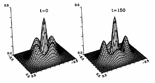
Figure 5.1: (a) Noise free stationary pattern as obtained from (5.1)-(5.2) and a stationary solution of (5.2) for $C>C_{A}$. (b) Configuration at time t=150 obtained from the stochastic evolution of the configuration in (a) with noise level $\epsilon=0.001$

The dynamics of symmetry restoring is described by the stochastic equation for $\eta$:

$$d_{t}\eta=cI_{1}{I_{2}-I_{3}\over\sqrt{I_{2}I_{3}}}\sin 4\delta+{1\over 4}({1\over\sqrt{I_{3}}}\xi^{{}^{\prime}}_{3}-{1\over\sqrt{I_{2}}}\xi^{{}^{\prime}}_{2}),$$ (5.4)

where $c$ is a constant proportional to the pump $C$, $I_{i}$=$|f_{i}|^{2}$ and $\xi^{{}^{\prime}}_{2,3}$ are real and independent Gaussian random processes. The drift part vanishes in the deterministic steady states. For those states, (5.4) describes a diffusive motion of $\eta$ (Wiener process) which is the basic physical mechanism of symmetry restoring. We also note that the pattern shown in Fig. (5.1) has four phase singularities in which $E(\rho,\varphi)=0$. These singular points also exhibit a diffusive motion [107].

The mechanism of symmetry restoring by phase diffusion also holds in systems which require a fully continuous description. If we consider a one dimensional system with a stationary pattern forming instability, the relevant pattern forming variable $\psi$ can be expressed, close to the instability, as [95]

$$\psi(x,t)=A(x,t)e^{iq_{M}x}+{\rm c.c.},$$ (5.5)

where $A=Re^{i\varphi}$ is the slowly varying amplitude of the most unstable mode $q_{M}$. Invariance under continuous space translations of the original problem ($x\rightarrow x+x_{0}$) implies gauge invariance under a change of a constant phase of the amplitude ($\varphi\rightarrow\varphi+\varphi_{0}$). Spontaneous symmetry breaking associated with pattern formation is here the choice of a particular phase of $A$, which means fixing a global position of the pattern by choosing among a continuous family of pattern forming solutions. The phase is the Goldstone mode associated with the broken symmetry, which generally satisfies a diffusion equation [109]: The linear evolution of longwavelength modulations of a pattern with dominant wave number $q+q_{M}$ is given by

$$\partial_{t}\varphi_{q}(x,t)=D(q)\partial^{2}_{x}\varphi_{q}(x,t)+\xi(x,t).$$ (5.6)

The Eckhaus instability [95, 110] is given by the wavenumber $q_{E}$ for which $D(q_{E})=0$. The condition $D(q)>0$ identifies the range of wave numbers around $q_{M}$ which give linearly stable patterns. Within the range of Eckhaus stable patterns, we have pure stochastic diffusion (no drift term) of the $k=0$ Fourier mode component of the phase $\varphi_{q}(x,t)$. For other $k$-modes we have damped phase fluctuations driven by the noise $\xi$. Such stationary phase fluctuations scale as $\langle\varphi^{2}(k)\rangle\sim k^{-2}$. The integral of $\langle\varphi^{2}(k)\rangle$ over all wave numbers diverges in spatial dimension $d<2$. Dimension $d=2$ is the critical dimension below which fluctuations associated with a broken continuous symmetry destroy long range order, or in other words symmetry is restored by noise. In our case this means that fluctuations in the local phase of the pattern preclude the existence of a rigidly ordered pattern with well defined wavenumber in a large system. We will now be more specific with these ideas in the example provided by the Swift-Hohenberg equation.

5.2 The stochastic Swift-Hohenberg equation: Symmetry restoring, pattern selection and noise modified Eckhaus instability.

The Swift-Hohenberg equation (SHE) was originally introduced to model the onset of a convective instability in simple fluids [111]. It describes the dynamical evolution of a scalar real variable $\psi(x,t)$,

$$\ \partial_{t}\psi(x,t) =[\mu-(1+\partial^{2}_{x})^{2}]\ \ \psi(x,t)-\psi^{3}(x,t)+\sqrt{\epsilon}\xi(x,t)=$$ (5.7)

$$=-{\delta F\over\delta\psi}+\sqrt{\epsilon}\xi(x,t),\ \$$ (5.8)

where we have explicitly indicated that the SHE has relaxational gradient dynamics determined by a Lyapunov functional $F$, and where $\xi(x,t)$ models thermal fluctuations as a Gaussian process with zero mean and

$$\langle\xi(x,t)\xi(x^{\prime},t^{\prime})\rangle=\delta(x-x^{\prime})\delta(t-t^{\prime}).$$ (5.9)

The study of the effect of thermal fluctuations in the onset of pattern formation $(\mu=0)$ was one of the original motivations in the study of the SHE [111, 112], but they were commonly neglected for some time because of its smallness for simple fluids. However, in several more recent experiments, in particular in the electrohydrodynamic instability in nematic liquid crystals, these fluctuations have been either directly or indirectly observed [102, 113].

In the absence of noise ($\epsilon=0$) and above threshold ($\mu>0$), the SHE admits stationary periodic solutions $\psi_{q}(x)$ characterized by a wavenumber $q$

$$\psi_{q}(x)=\sum_{i}A_{i}(q)\sin[(2i+1)qx]\ ,\ \ \ q_{-L}<q<q_{L}.$$ (5.10)

These solutions exist for a band of wavenumbers centered around $q=q_{M}=1$ with $q_{\pm L}=\sqrt{1\pm\sqrt{\mu}}$. These are linearly unstable wave numbers for the no pattern” solution $\psi=0$, being $q=q_{M}$ the most unstable mode. We emphasize that this mode does not coincide with the mode $q_{min}$ associated with the periodic solution which minimizes the potential $F$. Close to threshold one finds [109]

$$q_{min}\approx 1-{\mu^{2}\over 1024}.$$ (5.11)

Figure 5.2: Schematic position of the different wavenumbers mentioned in the text. The decay from an Eckhaus unstable wavenumber $q_{i}$ to a final wavenumber $q_{f}$ is also indicated

Stable periodic solutions only exist in a restricted band of wave numbers $q_{-E}<q<q_{E}$, where $q_{\pm E}$ are the critical wave numbers for the Eckhaus instability described above [114]. For small $\mu$, $q_{\pm E}\sim 1+(q_{\pm L}-1)/\sqrt{3}$, Fig. (5.2). An important fact about the Eckhaus instability in the SHE is that it is a subcritical bifurcation. Defining $V(q)=F[\psi_{q}(x)]$, the Eckhaus boundary is given by the wavenumbers such that ${\partial^{2}V(q)\over\partial q^{2}}=0$, so that $q_{E}$ plays the role of a spinodal line in first order phase transitions [46] separating unstable $(q_{L}>q>q_{E},q_{-L}<q<q_{-E})$ from metastable states $(q_{-E}<q<q_{E})$. The only globally stable state, in the presence of noise, is the one minimizing $F$. For further reference we also note that for the decay of a solution with wavenumber $q_{i}$ outside the Eckhaus stable range, the initially fastest growing mode is determined by a linearized analysis around a periodic solution $\psi_{q_{i}}(x)$ (Bloch eigenvalue problem). This fastest growing mode is no longer $q_{M}=1$ but $q_{M}(q_{i})$, a function of $q_{i}$.

We will now address three questions regarding the role of noise in the SHE. First is how noise destroys long range order, second the influence of noise in the dynamical process of pattern selection from a given initial condition, and finally how noise modifies the Eckhaus instability. Answers to these questions [115, 116, 117] are mostly found from extensive numerical simulations in which a system of size $L$, with periodic boundary conditions, is discretized in a grid of $N$ points $x_{i}$, with $N$ ranging from $1024$ to $8192$ points and a discretization step $\Delta x=L/N=2\pi/32$. For these sizes the number of changes of sign (NCS) of a periodic solution with $q=q_{M}$ ranges from $64$ to $512$, which identifies the number of convective rolls in the system.

Our general arguments above imply that there is no long range order in this one dimensional system when any amount of noise is present ( a discussion of the $d=2$ case is given in [118]). A quantitative measure of this statement can be given in terms of a stationary structure factor defined as

$$\lim_{t\rightarrow\infty}\ P(q,t)={1\over N}|\sum^{N}_{i=1}\psi(x_{i},t)e^{-iqx_{i}}|^{2}.$$ (5.12)

Alternatively one can look at the normalized correlation function

$$G(r)=\lim_{t\rightarrow\infty}{\langle\psi(x+r,t)\psi(x,t)\rangle\over\langle\psi(x,t)\rangle^{2}}.$$ (5.13)

The numerical results make explicit the absence of long range order in several ways. Consider first a single realization of the process, that is the stochastic evolution of a configuration $\psi(x,t)$. The long time dynamics is characterized by mode competition with no single dominant mode, so that no periodic solution is established. For small systems ($N=1024$) this is evidentiated by a power spectrum $P(q,t)$ which evolves in time with a hopping maximum wave number and a few modes being permanently excited by noise. The absence of a global wave number is also evidentiated by considering a local structure factor at a fixed time. Such local structure factor centered in $x_{0}$ is defined replacing in (5.11) $\psi(x_{i},t)$ by a filtered value around $x_{0}$: $\psi_{x_{0}}(x_{i},t)=e^{-(x_{i}-x_{0})^{2}/\beta^{2}}\psi(x_{i},t)$. The local structure factor $P_{x_{0}}(q,t)$, shown in Fig. (5.3), shows a well defined peak at a wave number that is a function of $x_{0}$. Therefore, $\psi(x,t)$ is locally periodic, but the local wave number varies from point to point. For large systems ($N=8192$) the structure factor of a configuration at a fixed time is broad, with a typical width of around 40 competing Fourier modes, which gives an idea of the range of coherence. In summary, configurations $\psi(x,t)$ cannot be characterized by a single wavenumber.

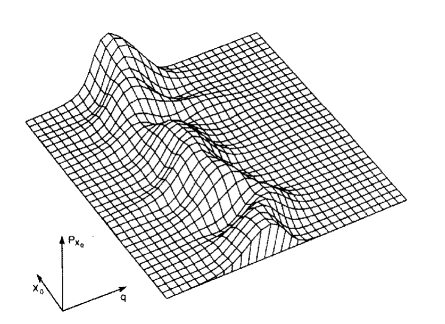
Figure 5.3: Local power spectrum $P_{x_{0}}(q,t)$ as defined in the text for a system of N=1024 points. Parameter values: $\mu=0.25$, $\beta=10$ and $\epsilon=0.2\Delta x$

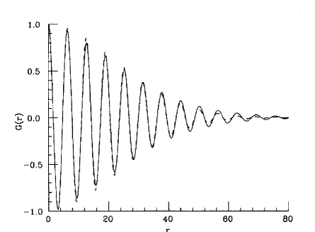
Figure 5.4: Solid line: Correlation function $G(r)\over{G(0)}$ obtained numerically as an average over 20 realizations for a system of N=8192 with parameter values $\mu=0.25$ and $\epsilon=0.1\Delta x$. Dashed line: fit to Eq. (5.13) with $q_{M}=1$ and $r_{0}=32$

Turning now to ensemble averages over several realizations, the stationary correlation function shown in Fig. (5.4), is well fitted by

$$G(r)=G(0)e^{-({r\over r_{0}})^{2}}cos(q_{M}r),$$ (5.14)

which identifies a correlation length $r_{0}$. For the typical parameter values of Fig. (5.4) we find $L/r_{0}\sim 50$ indicating that coherence in the pattern is only maintained in $1/50$ of the system size. The Fourier transform of the correlation function, or ensemble averaged power spectrum, requires a different fitting for the wings of the spectrum [115] and its width is found to grow linearly with noise intensity. We note that despite the absence of long range order, and therefore of a wavenumber for the system, still a conservation of the NCS holds during the stochastic steady state dynamics. Such conserved NCS can be used to define a global wave number or a mean periodicity of the system.

The question of pattern selection in this problem can be stated as which of the stable solutions $\psi_{q}(x)$ within the Eckhaus stable band is chosen from a given initial condition. Commonly proposed answers to this question are two: a) An argument based on relaxational dynamics on $F$ favor the selection of $q_{min}$. This is a potential argument based on the role of noise along the dynamical path. b) The argument of fastest linear growth favors the selection of $q_{M}$ since this solution is linearly stable, dominates in the early time dynamics, and there is conservation of NCS after the initial transient. Two simple comments are here in order. First is that, from a deterministic point of view, the selected state is entirely determined by initial conditions and any linearly stable state is reachable from an appropriate initial condition. Secondly is that, from the stochastic point of view, the question is ill-posed since we have shown that no single wavenumber characterizes the long time configurations. Still, the question makes sense if we ask for the global wave number corresponding to a selected NCS.

From this stochastic point of view one asks for a distribution of selected wavenumbers obtained as an ensemble average from a statistically distributed set of typical initial conditions. A natural situation to consider is the growth of the pattern from random initial conditions around $\psi=0$. This corresponds again to the case of the decay of an unstable state (discussed in Sect. 3), created by changing the control parameter $\mu$ from below ($\mu<0$) to above ($\mu>0$) the pattern forming instability. In this case the numerical solutions indicate that noise along path washes out the influence of the initial configuration. The final states are statistically distributed around the NCS corresponding to the global wavenumber $q_{M}$. However, the distribution is significantly narrower than the range of Eckhaus stable wavenumbers. Therefore the selected states are not uniformly distributed among all possible linearly stable states. The issue of selection of $q_{M}$ versus selection of $q_{min}$ cannot be clearly answered numerically because the two wavenumbers are numerically very similar. An alternative situation to address this question is to study the decay from a solution with wavenumber $q_{i}$ which is Eckhaus unstable, Fig. (5.2). Noise drives the system away from the initial condition and there is a transient in which the NCS changes, leading to a configuration with a final global wavenumber $q_{f}$. The time dependence of the NCS for a fixed $q_{i}$ and averaged over 20 realizations of the noise is shown in Fig. (5.5). It is seen that the evolution gets trapped in a metastable state after the disappearance of 72 rolls. The final observed NCS is consistent with the global wavenumber associated with fastest growth $q_{M}(q_{i})$, and it differs from $q_{min}$, which minimizes $F$, in another 36 rolls. Therefore, noise of moderate strength along the dynamical path is not able to drive the system, in the explored time scale, to the configuration which minimizes the Lyapunov functional of the problem, or equivalently to the most probable configuration in terms of the stationary solution of the Fokker-Planck equation associated with (5.7). The dynamical mechanism of pattern selection seems to be by the mode of fastest growth and this is robust against moderate fluctuations. Eventually, and for extremely long time scales, it is a rigorous mathematical statement that noise will induce jumps to configurations with a lower value of $F$. Of course, larger noise intensity would induce earlier jumps, but when the noise becomes larger, the conservation of NCS does not hold anymore, and the question of pattern selection becomes meaningless.

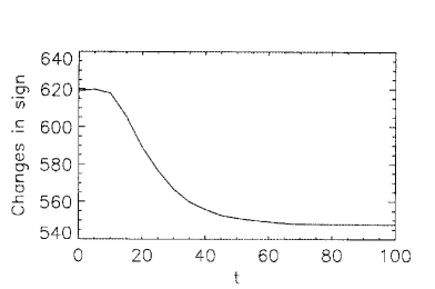
Figure 5.5: Time dependence of the averaged NCS in the decay of an Eckhaus unstable configuration for a system of N=8192 with $\mu=0.56$ and $\epsilon=0.1\Delta x$. NCS=512 corresponds to $q=1$

The fact that $q_{f}$ is given by the growth of fastest mode $q_{M}(q_{i})$ associated with the decay from $q_{i}$ breaks down when $q_{i}$ becomes close enough to the Eckhaus stability boundary $q_{\pm E}$. In this case one enters a fluctuation dominated regime in which $q_{f}$ can be identified neither with $q_{M}(q_{i})$ nor with $q_{min}$. We already mentioned that the Eckhaus boundary is similar to a spinodal line in the theory of phase transitions. It is well known in that context that such line is only a meanfield concept, so that it is not well defined when fluctuations are present [46]. A similar results hold here, and the Eckhaus boundary, when fluctuations are present, is only defined as an effective stability boundary for a time scale of observation [117].

To clarify this point we need first to characterize the range of $q_{i}$ for which we are in a fluctuation dominated regime. We can give a criterion which, being similar to the Ginzburg criterion of phase transitions [119], is based on the passage time ideas discussed in Sect. 3. The linearized analysis of the dynamics around a configuration $\psi_{q_{i}}(x)$ identifies a most unstable Bloch eigenmode $q_{M}(q_{i})$ with eigenvalue or linear growth rate $\lambda_{m}(q_{i})$. The amplitude $u$ of this mode satisfies during the early stages of decay a linear SDE

$$\dot{u}(t)=\lambda_{m}u(t)+\sqrt{\epsilon}\xi(t),$$ (5.15)

where $\xi(t)$ is a white Gaussian random process which results from the projection of $\xi(x,t)$ onto the most unstable Bloch eigenmode. Equation (5.14), that is the linear regime, is valid up to a time $T$ at which the amplitude $u$ becomes large enough, so that nonlinearities become important. This time is the MFPT calculated in Sect. 3:

$$T\sim{1\over 2\lambda_{m}}\ln({u_{0}^{2}\lambda_{m}\over\epsilon}),$$ (5.16)

where $u_{0}$ is a reference value for the amplitude $u$. We should now remember that the calculation of $T$ was based on the replacement of a stochastic process $h(t)$, that played the role of an effective initial condition, by a stationary random variable $h(\infty)$. This replacement was valid after a time $t_{m}\sim\lambda_{m}^{-1}$. The time scale given by $t_{m}$ is the fluctuation dominated regime in which $u(t)$ stays fluctuating around $u=0$. The existence of a linear growth regime invoked in our earlier discussion requires a separation of time scales between $t_{m}$ and $T$. If this is not satisfied we enter directly from a fluctuation dominated regime into the nonlinear regime, and the argument of fastest growing mode does not make further sense. The separation of time scales $t_{m}\ll T$ breaks down for

$$\lambda_{m}\approx{\epsilon\over u_{0}^{2}}.$$ (5.17)

Since it is possible to show that $\lambda_{m}\sim(q_{i}-q_{E})^{2}$, eq. (5.16) determines the range of initial wavenumbers $q_{i}$ close to $q_{E}$ for which a linear regime does not exist in the decay process. This is the regime dominated by fluctuations for which the definition $q_{E}$ of the Eckhaus boundary based on a linear deterministic analysis is not meaningful. A clear example of the consequences of this statement is provided by the numerical evidence that, for small noise amplitudes, periodic solutions with $q_{i}<q_{E}$ (within the linear deterministic Eckhaus stable band) are not maintained in time and decay to configurations with a global $q_{f}$ closer to $q=1$. In addition, for initial configurations within the fluctuation dominated regime in the Eckhaus unstable range one finds that the result $q_{f}=q_{M}(q_{i})$ does not longer hold.

Having argued that the Eckhaus boundary is not properly defined in the presence of fluctuations, we still can characterize a fluctuation shifted fuzzy boundary $\tilde{q}_{E}$ separating unstable from metastable states. Such boundary is defined with respect to a given long time scale of observation of the system. Within that scale of observation, it is defined as the value of $q_{i}$ for which a relaxation time diverges. Of course this is based on extrapolation of data for a range $\tilde{q}_{E}<q_{i}$ in which decay is observed. Numerical results indicate that $q_{f}$ becomes a linear function of $q_{i}$ so that $\tilde{q}_{E}$ can be identified by extrapolation to $q_{i}=q_{f}$. We further note that the nonlinear relaxation process in this fluctuation dominated regime exhibits a form of dynamical scaling [117].

We close this section with a final remark on pattern selection on nonrelaxational systems. There are pattern forming models that, as described in Sect. 4, do not follow a relaxational dynamics, but still can have a Lyapunov functional. An example recently considered is the Greenside-Cross equation in d=2 [123]. Our general discussion on pattern selection dynamics makes clear that the configuration minimizing a Lyapunov functional might not be the selected configuration in many cases. This has been shown here in the case of a purely relaxational dynamics and, a fortiori, will also be true for nonrelaxational dynamics.

5.3 Noise amplification in convective instabilities: Noise sustained structures

Generally speaking, we call a state of a system absolutely unstable if a perturbation localized around a spatial position grows in time at that spatial position. A state is absolutely stable if the perturbation decays in time. An intermediate situation occurs at a convectively unstable state: A local perturbation grows in time but traveling in the system, so that the perturbation decays in time at fixed space positions but, being convected away from the place where it originated, grows in time in the frame of reference that moves with the perturbation. The role of noise in a convectively unstable situation is very important [121] because, as it happened in the decay of an unstable state, there is a mechanism of noise amplification: If what grows at the instability is some sort of spatial structure (wave or pattern), this structure will not be seen at steady state in the absence of noise because any perturbation is convected away and leaves the system. However, if noise is continuously present in the system, it will be spatially amplified and a persistent structure sustained by noise will be observed. Important questions in this context are the determination of conditions for the existence of a convectively unstable regime, the characterization of a noise sustained structure and the characterization of the threshold for the transition between a noise sustained structure and a deterministically sustained structure.

As an example of this situation we consider the complex Ginzburg Landau Equation (CGLE) which is the amplitude equation for the complex amplitude $A$ of the dominating mode at a Hopf bifurcation in a spatially extended system [95]. Using a different notation than in Sect. 4,

$$\partial_{t}A(x,t)-v\partial_{x}A(x,t)=\mu A(x,t)+(1+i\alpha)\partial_{x}^{2}A(x,t)-(1+i\beta)|A(x,t)|^{2}A(x,t)+\sqrt{\varepsilon}\xi(x,t)$$ (5.18)

For $v=0$ the state $A=0$ changes from absolutely stable to absolutely unstable when the control parameter changes from $\mu<0$ to $\mu>0$. Linearly stable traveling waves exist as solutions of the CGLE for $\mu>0$ and $1+\alpha\beta>0$. The convective term $v\partial_{x}A(x,t)$ becomes important when boundary conditions are such that it can not be eliminated by a change of frame of reference. To understand the role of this term we linearize (5.17) around $A=0$. The complex dispersion relation $\omega$ for a disturbance of wavenumber $K$, that thus behaves as $e^{\omega t+Kx}$, becomes:

$$\omega=\mu+Kv+(1+i\alpha)K^{2}\quad,\quad K=k+iq\quad,$$ (5.19)

and the growth rate of such a perturbation is given by $Re\omega(K)$. Using the method of steepest descent, the long-time behavior of the system along a ray defined by fixed $x/t$, i.e. in a frame moving with a velocity $v_{0}=x/t$, is governed by the saddle point defined by :

$$Re\left(\frac{d\omega}{dK}\right)=v_{0}\quad,\quad Im\left(\frac{d\omega}{dK}\right)=0.$$ (5.20)

Since absolute instability occurs when perturbations grow at fixed locations, one has to consider the growth rate of modes evolving with zero group velocity, which are defined by:

$$Re\left(\frac{d\omega}{dK}\right)=Im\left(\frac{d\omega}{dK}\right)=0$$ (5.21)

These conditions define the following wave number

$$q=-\alpha k\quad,\quad k=-\frac{v}{2(1+\alpha^{2})}\quad.$$ (5.22)

The real part of $\omega$, which determines the growth rate $\lambda$ of these modes is then:

$$\lambda=Re(\omega)=\mu-\frac{v^{2}}{4(1+\alpha^{2})}\quad.$$ (5.23)

Therefore, the uniform reference state $(A=0)$ is absolutely unstable if $\lambda>0$. This condition determines a critical line in the parameter space which can be expressed for the group velocity $v$ or the control parameter $\mu$ as

$$v_{c}=2\sqrt{\mu(1+\alpha^{2})}\qquad\mbox{or}\qquad\mu_{c}=\frac{v^{2}}{4(1+\alpha^{2})}\quad.$$ (5.24)

Hence, for $0<\mu<\mu_{c}$, the uniform reference state is convectively unstable, and wave patterns are convected away in the absence of noise. For $\mu>\mu_{c}$, wave patterns may grow and are sustained by the dynamics, even in the absence of noise.

This analysis of the convective instability in the CGLE has been used [122] to account for the corresponding experimental situation in the case of a Taylor-Couette system with through flow, where the transition from convective to absolute instability and noise sustained structures are observed. Noise sustained structures in the convectively unstable regime $\mu<\mu_{c}$ can be characterized by the stochastic trajectory of $A$ at a fixed space point. It is seen that the statistical properties can be explained in terms of a stochastic phase diffusion for the phase of $A$, while $|A|$ shows small fluctuations. This identifies again a structure with no long range order since it is being excited by noise. An equivalent quantitative measure of the phase diffusion wandering induced by noise amplification is given by the width of the frequency power spectrum of $A$ at a fixed point. This spectrum is broad in the convectively unstable regime. The threshold at $\mu=\mu_{c}$ can be characterized by the way in which the width of the spectrum vanishes (divergence of a correlation time) as one moves from the convectively unstable regime to the absolute unstable regime. In the latter regime the structure persists for vanishing noise and the spectrum is essentially noise free.

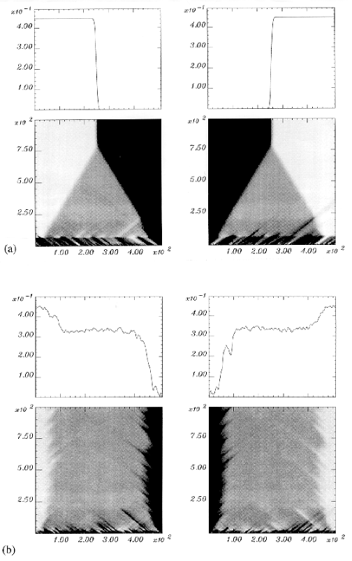
Figure 5.6: Space (horizontal axis)-time (vertical axis) grey scale plot of the moduli of the amplitudes $A(x,t)$ (left) and $B(x,t)$ (right) for $\gamma=0.8$, $\mu=0.408$, $v=1$, $\alpha=0.02$, $\beta=0.04$, $\delta=0.05$. The upper diagrams show the spatial dependence of $|A|$ and $|B|$ at the end of the space-time plots. (a) Deterministic case ($\epsilon=0$): the disturbances of the initial random pattern create initially a standing wave pattern which is replaced, due to front propagation, by a symmetric traveling wave pattern. (b) Stochastic case ($\epsilon=10^{-4}$): the spatially distributed noise gives rise, in the bulk of the system, to a noise sustained wave structure fluctuating around the deterministic value

These ideas have been recently extended [124] to the case of two coupled CGLE which describe a system undergoing a Hopf bifurcation at a finite wave number. The amplitudes $A$ and $B$ of the two emerging counterpropagating waves satisfy

$$\partial_{t}A(x,t)-v\partial_{x}A(x,t) = \mu A(x,t)+(1+i\alpha)\partial_{x}^{2}A(x,t)-(1+i\beta)|A(x,t)|^{2}A(x,t)$$ (5.25)

$$- (\gamma+i\delta)|B(x,t)|^{2}A(x,t)+\sqrt{\varepsilon}\xi_{A}(x,t)$$

$$\partial_{t}B(x,t)+v\partial_{x}B(x,t) = \mu B(x,t)+(1+i\alpha)\partial_{x}^{2}B(x,t)-(1+i\beta)|B(x,t)|^{2}B(x,t)$$ (5.26)

$$- (\gamma+i\delta)|A(x,t)|^{2}B(x,t)+\sqrt{\varepsilon}\xi_{B}(x,t).$$

For $\gamma>1$ there is strong coupling of the two waves, so that only one of them survives, and the situation is the same than for the single CGLE. For $\gamma<1$ a stability analysis analogous to the one discussed for the single CGLE shows that the Traveling Wave solution (TW), $A\not=0$, $B=0$, is convectively unstable for $\mu_{c}<\mu<\frac{\mu_{c}}{1-\gamma}$, while it becomes absolutely unstable for $\frac{\mu_{c}}{1-\gamma}<\mu$. Therefore, this deterministic analysis would imply that TW solutions are observed while they are convectively unstable and Standing Wave solutions (SW), $A=B\not=0$, emerge when crossing the line

$$\gamma_{c}=1-{\mu_{c}\over\mu}=1-\frac{v^{2}}{4\mu(1+\alpha^{2})},$$ (5.27)

and getting into the region in which the TW solution is absolutely unstable. However, from a stochastic point of view one expects that for $\gamma>\gamma_{c}$ (TW convectively unstable) noise will be amplified so that the two amplitudes $A$ and $B$ become nonzero and a noise sustained SW emerges. Crossing the line $\gamma=\gamma_{c}$ would then lead from a noise sustained SW to a deterministically sustained SW. Evidence for the noise sustained SW for $\gamma>\gamma_{c}$ is shown in Fig. (5.6), where the results of a numerical simulation with and without noise are shown. Initial conditions are random fluctuations around the state $A=B=0$ and the boundary conditions used in a system of size $L$ are

$$A(L,t)=0\quad,\quad B(0,t)=0\quad,\quad\partial_{x}A(0,t)=0\quad,\quad\partial_{x}B(L,t)=0\quad.$$ (5.28)

The transition at $\gamma=\gamma_{c}$ can be characterized in terms of the width of the frequency power spectrum $|A(x,\omega)|^{2}$ of $A$ at a fixed space point (inverse correlation time) or by the width of the time average of the power spectrum $|A(k,t)|^{2}$ (inverse correlation length). The two power spectra are broad in the region of noise sustained SW. The onset of the deterministic SW is identified by a divergence of the correlation time and a correlation length becoming of the order of the system size (for the relatively small sizes explored). However the transition does not occur at $\gamma=\gamma_{c}$ but at a slightly noise-shifted value [124]. This is just another example of instability point shifted and modified by noise as the one described above for the Eckhaus instability and the shifting of the phase transition point discussed in Sect 6.

6 Fluctuations, phase transitions and noise–induced transitions

In many cases, as we have encountered in previous examples, noise has a disordering effect. In this section, however, we consider a class of problem in which noise acts in a non trivial and unexpected way inducing a phase transition to an ordered state in spatially distributed system [125, 126, 127]. We first review the transitions induced by noise in the zero–dimensional case and then turn to the extended systems.

6.1 Noise–induced transitions

Noise induced transitions have been known for some time now [128]. Let us start with a simple example: consider the following SDE with multiplicative noise (Stratonovich sense)

$$\dot{x}=f(x)+g(x)\xi(t)$$ (6.1)

$\xi(t)$ is a white noise process with mean value zero and correlations:

$$\langle\xi(t)\xi(t^{\prime})\rangle=\sigma^{2}\delta(t-t^{\prime})$$ (6.2)

The parameter $\sigma$ is called the noise intensity and, although it could be absorbed in the function $g(x)$, is included here to stress the fact that when $\sigma=0$ the noise effectively disappears from the problem. By solving the Fokker–Planck equation, one can check that the stationary distribution is given by:

$$P_{st}(x)=C\exp\left\{\int_{0}^{x}dy\frac{f(y)-{\sigma^{2}\over 2}g(y)g^{\prime}(y)}{{\sigma^{2}\over 2}g^{2}(y)}\right\}$$ (6.3)

Consequently, the extrema $\bar{x}$ of the stationary distribution are given by:

$$f(\bar{x})-\frac{\sigma^{2}}{2}g(\bar{x})g^{\prime}(\bar{x})=0$$ (6.4)

And, quite generally, they will be different from the fixed points of the deterministic dynamics, $\sigma=0$. It is possible, then, that new stationary states appear as a consequence of the presence of the noise term. Let us consider a specific case:

$$\dot{x}=-x+\lambda x(1-x^{2})+(1-x^{2})\xi(t)$$ (6.5)

for $|x|<1$ and $\lambda<1$. It can be put in the form:

$$\dot{x}=-\frac{\partial V}{\partial x}+(1-x^{2})\xi(t)$$ (6.6)

with

$$V(x)=\frac{1-\lambda}{2}x^{2}+\frac{\lambda}{4}x^{4}$$ (6.7)

In the absence of noise, $\sigma=0$, the deterministic problem has a unique fixed stable point at $x=0$. For small $\sigma$ the situation is somewhat similar, the stationary probability distribution is peaked around the value $x=0$. However, by increasing the noise intensity, namely for $\sigma^{2}>2\lambda$, the stationary probability distribution changes shape and becomes bimodal. This change from a unimodal to a bimodal distribution obtained by increasing the noise intensity has been called a noise–induced transition . Of course, this can not be identified as a true “phase transition”, because during the stochastic evolution the system will jump many times from one maximum of the probability to the other, thus not breaking ergodicity, which is a clear signature of a phase transition. We show in Fig.(6.1) how noise is capable of restoring the symmetry and, on the average the “order parameter”, $m\equiv\langle x\rangle=0$. One would think that, in similarity to what happens in other models of statistical mechanics, it should be possible to obtain a phase transition by coupling many of these systems. The coupling should favor the ordering of neighboring variables to a common value. The system would, then, choose between one of the two maxima displaying a macroscopic not vanishing order parameter. However, it turns out that, although the noise is effectively capable of inducing a phase transition, it does so in a different way.

Figure 6.1: Typical trajectory coming from a numerical solution of the SDE (6.5). We see that, although there are two preferred values, $\pm x_{0}$, for the variable $x$ (i.e. the stationary distribution is bimodal), there are many jumps between these two preferred values. If one were to interpret $+x_{0}$ and $-x_{0}$ as two “phases” of the system, we would conclude that noise is capable of restoring the symmetry between these two phases. Values of the parameters are $\lambda=0.5$, $\sigma^{2}=2$.

6.2 Noise–induced phase transitions

Remember that for relaxational systems noise has the effect of introducing fluctuations around the minima of the potential. If the potential is bistable and the noise intensity becomes large enough, the system is brought out of the minima in a short time scale and the order parameter vanishes. One can interpret these results in terms of a shift in the transition. Let us be more specific: consider the Ginzburg–Landau model [130, 131] (model $A$ in the taxonomy of [87], also called the $\varphi^{4}$ model). We consider the lattice version: the variables $x_{i}$ follow the relaxational gradient evolution equations:

$$\dot{x}_{i}=-\frac{\partial V(x)}{\partial x_{i}}+\xi_{i}(t)$$ (6.8)

The index $i$ runs over the $N=L^{d}$ sites of a $d$–dimensional regular lattice (of lattice spacing $\Delta r=1$). The potential is:

$$V(x)=\sum_{i=1}^{N}\left[-\frac{b}{2}x_{i}^{2}+\frac{1}{4}x_{i}^{4}+\frac{1}{2}|\vec{\nabla}x_{i}|^{2}\right]$$ (6.9)

We use the simplest form for the lattice gradient $\vec{\nabla}x_{i}$. It is such that its contribution to the dynamical equations is the lattice–Laplacian:

$$-\frac{\partial}{\partial x_{i}}\left[\sum_{j}|\vec{\nabla}x_{j}|^{2}\right]=2\sum_{j\in n(i)}(x_{j}-x_{i})$$ (6.10)

the sum over the index $j$ runs over the set $n(i)$ of the $2d$ lattice sites which are nearest neighbors of site $i$.

As discussed in Sect. 4.2, if the noise term satisfies the fluctuation–dissipation relation:

$$\langle\xi_{i}(t)\xi_{j}(t^{\prime})\rangle=2k_{B}T\delta_{ij}\delta(t-t^{\prime})$$ (6.11)

the stationary distribution of (6.8) is given by:

$$P_{s}t(x)=Z^{-1}\exp[-V(x)/k_{B}T]$$ (6.12)

$Z$ being a normalization constant (the partition function). The parameter $b$ also depends on temperature $b=b(T)$ and is such that changes sign at $T=T_{0}$, being positive for $T<T_{0}$ and negative for $T>T_{0}$. If we neglect thermal fluctuations, the stationary distribution becomes a sum of delta functions centered around the minima of the potential $V(x)$. If $b<0$, the potential has a single minimum and if $b>0$ the potential has two minima. In these minima all the variables $x_{i}$ adopt a common value $m$. The order parameter is:

$$m=\left\{\begin{array}[]{lll}0&b<0&,T>T_{0}\\ \pm\sqrt{b}&b>0&,T<T_{0}\end{array}\right.$$ (6.13)

This is nothing but a simple example of Landau theory of phase–transitions [132]. The two minima, corresponding to the $\pm$ signs in the order parameter, are the two phases whose symmetry is broken by the time evolution. In the absence of noise, there is no mechanism to jump from one minimum to the other.

If we now go beyond Landau’s mean field approximation, we include thermal fluctuations by explicitly considering the noise term. Without going into details [130, 131, 133], we can understand that fluctuations make it possible for the system to jump from one minimum to the other, hence restoring the symmetry. For this to happen, the thermal energy $k_{B}T$ must be of the order of the energy barrier separating the two minima. Put in another way: when thermal fluctuations are taken into account, one needs a deeper potential in order to keep the broken symmetry. Or still in other words: when fluctuations are included, there is a shift in the location of the phase transition from $b=0$ to $b>0$, what implies that the new critical temperature is smaller than the Landau mean–field temperature, see Fig. (6.2). We conclude that the probability distribution for the order parameter changes from bimodal to unimodal when increasing the fluctuations (noise intensity). In fact, for this change to happen at temperature greater than zero, one needs the spatial dimension to be strictly greater than $1$, $d>1$ (lower critical dimension of the $\varphi^{4}$ model).

Figure 6.2: Order parameter $m$ for the $\varphi^{4}$ model of phase transitions as a function of the parameter $b$. The continuous line is Landau’s solution, eq. (6.13); it has a critical point at $b=0$. The dotted line is the (schematic) exact result (when including thermal fluctuations) for spatial dimension $d>1$. Notice that there is a shift in the transition when including fluctuations towards larger values for $b$, smaller temperatures.

We have witnessed in the case of zero–dimensional (one variable) models, how fluctuations can actually go the other way and induce a bimodal distribution when increasing the noise intensity. We called this a noise–induced transition. In order to have a real noise–induced phase transition, we guess that we need to go a spatially extended system. The role of multiplicative noise in spatially extended systems in the context of phase transitions [44, 125, 126, 127] and pattern–forming instabilities [134, 135, 136] has been thoroughly studied. We consider here the $d$–dimensional version of (6.1) with the inclusion of nearest neighbor coupling terms:

$$\dot{x}_{i}=f(x_{i})+\frac{D}{2d}\sum_{j\in n(i)}(x_{j}-x_{i})+g(x_{i})\xi_{i}(t)$$ (6.14)

The parameter $D>0$ measures the strength of the coupling between neighboring sites. The noise variables $\xi_{i}(t)$ are Gaussian distributed of zero mean and correlations given by:

$$\langle\xi_{i}(t)\xi_{j}(t^{\prime})\rangle=\sigma^{2}\delta_{ij}\delta(t-t^{\prime})$$ (6.15)

We skip now some of the mathematical details. Although it is possible to write down the Fokker–Planck equation for the joint probability distribution function $P(x_{1},\dots,x_{N};t)$, corresponding to this set of stochastic differential equations, it is not possible now, as it was in the zero–dimensional case, to solve it in order to find the stationary distribution $P_{st}(x_{1},\dots,x_{N})$. What one does, though, is to obtain an exact equation for the one–site probability $P_{st}(x_{i})$:

$$\frac{\partial}{\partial x_{i}}\left[-f(x_{i})+D[x_{i}-\langle x_{n(i)}|x_{i}\rangle]+\frac{\sigma^{2}}{2}g(x_{i})\frac{\partial}{\partial x_{i}}g(x_{i})\right]P_{st}(x_{i})=0$$ (6.16)

In this equation appears the conditional mean value $\langle x_{n(i)}|x_{i}\rangle$: the mean value of a neighbor site of $i$ given that the random variable $x_{i}$ takes a fixed value. In order to proceed, we make now a mean–field type assumption. This approximation, close in spirit to Weiss mean–field theory for ferromagnetism [13], consists in the assumption that the above conditional mean value is equal to the mean value of $x_{i}$ itself:

$$\langle x_{n(i)}|x_{i}\rangle=\langle x_{i}\rangle$$ (6.17)

It is possible now to integrate out all the variables except a given one, say $x_{1}$, from equation (6.16) to obtain a closed equation for $P_{st}(x_{1})$ whose solution is (we have dropped the subindex $1$ for the sake of simplicity and because similar equations are satisfied for any $x_{i}$):

$$P_{st}(x)=Z^{-1}\exp\left[\int^{x}dy\frac{f(y)-\frac{\sigma^{2}}{2}g(y)g^{\prime}(y)-D(y-\langle x\rangle)}{{\sigma^{2}\over 2}g^{2}(y)}\right]$$ (6.18)

In this equation, the unknown value $\langle x\rangle$is then obtained by the consistency relation:

$$\langle x\rangle=\int dxP_{st}(x)$$ (6.19)

The solutions of equations (6.18) and (6.19) are to be considered the order parameter, $m=\langle x\rangle$. These equations can be solved numerically, but a first clue about the possible solutions can be obtained in the limit $D\to\infty$ by means of a saddle–point integral, which yields:

$$f(\langle x\rangle)+\frac{\sigma^{2}}{2}g(\langle x\rangle)g^{\prime}(\langle x\rangle)=0$$ (6.20)

If by varying the noise intensity, $\sigma$, the order parameter changes from $m=0$ to a non–zero value, we interpret this as a phase transition. In the example given below, we will show that the main features of a true phase transition hold, namely: the breaking of ergodicity, the divergence of correlations, the validity of scaling relations, etc. [120]. Finally, note the difference in sign of this equation with equation (6.4) giving the maxima of the probability distribution in the case of noise–induced–transitions. This means that, at least in the limit of very strong coupling in which equation (6.20) holds, those systems displaying a noise–induced transition will not show a noise–induced phase transition and viceversa.

Figure 6.3: Numerical solution of equations (6.18) and (6.19) for the model (6.21) showing the regions of order and disorder (solid line). The dotted line is the result of a higher order approximation (not explained in the main text) which goes beyond the approximation (6.17) by including correlations amongst nearest neighbors variables.

A simple model is obtained by choosing [125, 126]:

$$\begin{array}[]{rcl}f(x)&=&-x(1+x^{2})^{2}=-\frac{\partial V}{\partial x},\hskip 28.45274ptV(x)=\frac{1}{3}(1+x^{2})^{3}\\ g(x)&=&1+x^{2}\end{array}$$ (6.21)

Let us summarize some properties of this model:
(i) For the deterministic version (no noise, $\sigma=0$) it is a relaxational gradient system with a potential $V(x)$ which displays a single minimum. Therefore, the stationary solution is $x_{i}=0$ for all $i$.
(ii) For the zero-dimensional version, in which there is no coupling between the different lattice points, $D=0$, each variable becomes independent of the others. By looking at the solutions of (6.4), one can check that this system does not present a noise–induced transition. Therefore, the stationary probability distribution $P_{st}(x_{i})$ has a maximum at $x_{i}=0$ again for all values of $i$, and is symmetric around $x=0$, hence, $m=\langle x_{i}\rangle=0$.
(iii) When both coupling and noise terms are present, $D\neq 0$, $\sigma\neq 0$, the stationary distribution has maxima at non–vanishing values of the variable. Due to the symmetry $x\to-x$, these maxima are at values $\pm x_{0}$, for some $x_{0}$. In fact, in the infinite coupling limit, equation (6.20) yields for the (common) average value:

$$m=\langle x\rangle=\pm\sqrt{\sigma^{2}-1}$$ (6.22)

This existence of a non–vanishing order parameter is also maintained at finite values for the coupling $D$, although then the consistency relation (6.19) must be solved numerically. In Fig. (6.3) we show the regions in parameter space for which this mean–field approach predicts a non–zero value of the order parameter. When the only solution is $\langle x\rangle=0$ we talk about a disordered phase, whereas when non–null solutions $\langle x\rangle\neq 0$ appear, we say that the system is in an ordered phase. Notice that, according to Fig. (6.3), an ordered phase can appear only for a sufficiently large value of the coupling parameter $D$ and within a range of values of the noise intensity $\sigma$, i.e. the transition is reentrant with respect to the noise intensity.

Figure 6.4: Phase diagram of the system defined by equations (6.14) and (6.21) for spatial dimension $d=2$. The dotted line is the result of the mean field approximation (independent of dimension). The symbols are the results of numerical simulations for different system sizes (from $L=16$, crosses, to $L=128$, squares). In this case the order parameter is defined as $m\equiv\langle|N^{-1}\sum_{i=1}^{N}x_{i}|\rangle$.

This prediction of the existence of a phase transition in the model of equations (6.21) has been fully confirmed by numerical simulations of the coupled set of Langevin equations (6.14) in the two–dimensional, $d=2$, case. The numerical solution has used appropriate versions of the Milshtein and Heun algorithms, see Sect. (2.4.4). We now describe some observed features of the transition as obtained from the computer simulations.

(i) First of all, there is the breaking of ergodicity. Due to the above mentioned symmetry $x\to-x$ and depending on initial conditions and white noise realizations, some realizations will go to positive values of the order parameter and some other to negative values. However, and this is the key point, the jumps between positive and negative values do not occur very often, and the frequency of the jumps strongly decreases with system size $N$, suggesting that in the limit $N\to\infty$ noise is not capable of restoring the symmetry.

Figure 6.5: Susceptibility $\hat{\chi}$ plotted as a function of the noise intensity $\sigma^{2}$. The symbols are the results of numerical simulations for different system sizes (same symbols meaning as in Fig. (6.4). Notice the sharp increase of the susceptibility as the system size increases, as usual in second–order phase transitions.

(ii) The second point is the existence of the transition. This is shown in Fig. (6.4) where we plot the order parameter as a function of noise intensity $\sigma$ for a value $D=20$ of the coupling parameter. According to Fig. (6.3) there should be a non–zero value for the order parameter for $1.1<\sigma^{2}<19.9$, approximately. Although the reentrant transition occurs at a value $\sigma^{2}\approx 6.7$, lower than the predicted in mean field, $\sigma^{2}\approx 19.9$, it is clear the increase of the order parameter from $m=0$ to a non–zero value and the further decrease towards $0$ through what appears to be two genuine second–order phase transitions. Of course, calling this a second–order phase transition is an abuse of language, since there is no free energy whose second derivatives show some degree of non–analiticity. Still we keep this name because, as we will see in the next paragraphs, many of the characteristics associated to a thermodynamic second–order phase transition are also present in this model.

(iii) In a second–order phase transition, the susceptibility diverges. Here we have defined a “susceptibility”, $\hat{\chi}$, as the following measure of the fluctuations of the order parameter:

$$\hat{\chi}\equiv\frac{\langle m^{2}\rangle-\langle m\rangle^{2}}{N\sigma^{2}}$$ (6.23)

(the presence of the $\sigma^{2}$ term is reminiscent of the statistical mechanics relation $\chi\equiv[\langle m^{2}\rangle-\langle m\rangle^{2}]/(Nk_{B}T)$ since in our model the equivalent of temperature $T$ is the noise intensity $\sigma^{2}$). In Fig. (6.5) we can see how the susceptibility develops maxima at the two transitions, maxima that increase with increasing system size, suggesting again a true non-analytical behavior (divergence) in the thermodynamic limit. It is possible to analyze these results in terms of finite size scaling relations, as shown later.

(iv) Another feature of a second–order phase transition is that of the long–range correlations. This is shown in Fig. (6.6) in which we plot the spatial correlation function $C(n)\equiv\langle(x_{i}-\langle x_{i}\rangle)(x_{i+n}-\langle x_{i+n}\rangle)\rangle$. Far from the two transition points, the correlation function decays very fast, but near both critical points, correlations decay very slowly. The same phenomenon has been observed for the correlation times (critical slowing down).

Figure 6.6: Correlation function $C(n)\equiv\langle(x_{i}-\langle x_{i}\rangle)(x_{i+n}-\langle x_{i+n}\rangle)\rangle$ for $D=20$ and three different values of the noise intensity $\sigma^{2}=1.65$ (solid line), $\sigma^{2}=4$ (dotted line), $\sigma^{2}=6.7$ (dashed line). Note that at the two critical points, the correlation function decays very slowly.

(v) Finally, we show now that the transition also satisfies the usual scaling relations valid in second order transitions. We have focused just in finite–size–scaling relations [137] (so useful for analysing the results of computer simulations [138, 139]). Although these finite–size scaling relations hold very generally for the model introduced in this section, we present results for the order parameter. According to finite size scaling theory, the order parameter should behave close enough to the critical points as:

$$m(\epsilon,L)=L^{-\beta/\nu}m(\epsilon L^{1/\nu})$$ (6.24)

where $\epsilon=1-\sigma^{2}/\sigma_{c}^{2}$ (for thermal phase transitions, this is defined as $\epsilon=1-T/T_{c}$, $T$ being the system temperature). The meaning of $\beta$ and $\nu$ is that of the usual scaling exponents. In Fig. (6.7) we plot $L^{\beta/\nu}m(\sigma,L)$ versus $L^{1/\nu}(1-\sigma^{2}/\sigma_{c}^{2})$ to show that curves corresponding to different values of $L$ and $\sigma$ fall onto a master curve, so confirming the validity of scaling. In this curve we have used the values of the $2$–$d$ Ising model exponents, $\nu=1$, $\beta=1/8$. Our data, then, suggests that this transition belongs to the $2$–$d$ Ising model universality class, although more precise data are needed in order to clarify this important point.

As a conclusion, we have shown in this section how the noise can have a different effect that it is usually accepted for Statistical Mechanics systems: it can induce long–range order in a spatially extended system. Recent extensions of this work have considered the effect of colored noise [140]. This is motivated because one expects that the kind of fluctuations leading to multiplicative noise will show a finite correlation time. The role of colored noise in the $\varphi^{4}$ model (with additive noise) has been studied in [141, 142] showing that a non–equilibrium phase transition can be induced by varying the correlation time $\tau$ of the noise. For zero–dimensional systems, a reentrant transition has been found in a noise–induced transition as a consequence of the color [143]. When multiplicative colored noise is included in an extended system, several new effects can appear. One of the most counter–intuitive ones being that of the disappearance of the order when increasing the coupling between nearest neighbor fields [140]. It is hoped that these recent theoretical developments can boost experimental work in the search for those predicted phenomena.

Figure 6.7: Plot of $L^{\beta/\nu}m(\sigma,L)$ versus $L^{1/\nu}(1-\sigma^{2}/\sigma_{c}^{2})$ with $\sigma_{c}^{2}=1.65$ for different system sizes (same symbols than in Fig. (6.3)), to show that the finite–size scaling relation (6.24) is well satisfied.

ACKNOWLEDGEMENT: We acknowledge partial financial support from DGICYT (Spain) projects PB94-1167 and PB94-1172 and from the European Union TMR project QSTRUCT (FMRX-CT96-0077). Our knowledge on this subject has been built through research work in collaboration with many colleagues and collaborators reported in the references below.

References

- [1] N. G. van Kampen, Stochastic Processes in Physics and Chemistry, North–Holland (1981).
- [2] C.W. Gardiner, Handbook of Stochastic Methods, Springer-Verlag, Berlin (1985).
- [3] H. Risken, The Fokker Planck Equation, Springer-Verlag, Berlin (1984).
- [4] W. Horsthemke and R. Lefever, Noise–Induced Transitions: Theory and Applications in Physics, Chemistry and Biology, Springer-Verlag, Berlin (1984).
- [5] Noise in Nonlinear Dynamical Systems, vols. 1, 2 and 3, Eds. F. Moss and P. V. E. McClintock, Cambridge University Press, Cambridge (1989).
- [6] H.S. Wio, An Introduction to Stochastic Processes and Nonequilibrium Statistical Physics, World Scientific (1994).
- [7] H. S. Wio, P. Colet, M. San Miguel, L. Pesquera and M. San Miguel, Phys. Rev. 40, 7312 (1989).
- [8] R. Benzi, A. Sutera and A. Vulpiani, J. Phys. A 14, L453 (1981); K. Wiesenfeld and F. Moss, Nature 373,33 (1995); Proc. NATO ARW on Stochastic Resonance in Physics and Biology, J. Stat. Phys. 70 (1993).
- [9] C. R. Doering, W. Horsthemke and J. Riodan, Phys. Rev. Lett. 72, 2984 (1994); J. Maddox, Nature 368, 287 (1994); S. M. Bezrukov and I. Vodyanoy, Nature 378, 362 (1995).
- [10] N. Wax, ed, Selected Papers on Noise and Stochastic Processes, Dover, New York (1954).
- [11] J. A. McLennan, Introduction to Non–Equilibrium Statistical–Mechanics, Prentice Hall (1989).
- [12] S.G. Brush, Kinetic Theory, Pergamon, Oxford (1966).
- [13] R.K. Pathria, Statistical Mechanics, Pergamon Press (1972).
- [14] L. Boltzmann, Ann. der Physik 57, 773 (1896) (reprinted in [12]); quoted by J. Lebowitz in 25 Years of Non–Equilibrium Statistical Mechanics, J.J. Brey, J. Marro, J.M. Rubí and M. San Miguel eds, Springer-Verlag (1995).
- [15] W. Feller, An Introduction to Probability Theory and its Applications, vols. 1,2. John Wiley & Sons (1971).
- [16] A. Papoulis, Probability, Random Variables, and Stochastic Processes, McGraw–Hill (1984).
- [17] G.H. Weiss, Aspects and Applications of the Random Walk, North–Holland (1994).
- [18] R.F. Fox, Phys. Rep. C48, 171 (1979).
- [19] M. Abramowitz and I.A. Stegun, Handbook of Mathematical Functions, Dover Publications (1972).
- [20] K. Falconer, Fractal Geometry, John Wiley and Sons (1990).
- [21] J.M. Sancho, M. San Miguel, S.L. Katz and J.D. Gunton, Phys. Rev. A26, 1589 (1982).
- [22] P. Hänggi, in Stochastic Processes Applied to Physics, L. Pesquera and M.A. Rodríguez, eds. World Scientific, Philadelphia (1985), pp.69-95.
- [23] R. Balescu, Equilibrium and Non–Equilibrium Statistical Mechanics, John Wiley and Sons (1975).
- [24] E.A. Novikov, Zh. Eksp. Teor. Fiz. 47, 1919 (1964) [Sov. Phys. JETP, 20, 1290 (1965)].
- [25] J.M. Sancho and M. San Miguel in volume 1 of [5].
- [26] T.C. Gard, Introduction to Stochastic Differential Equations, Marcel Dekker, vol 114 of Monographs and Textbooks in Pure and Applied Mathematics (1987).
- [27] A. Greiner, W. Strittmatter and J. Honerkamp, J. Stat. Phys. 51, 95 (1988).
- [28] P.E. Kloeden and E. Platen, Numerical Solution of Stochastic Differential Equations, Springer-Verlag (1992).
- [29] F. James, Comp. Phys. Comm. 60, 329 (1990).
- [30] D.E. Knuth, The Art of Computer Programming, vol.2 Seminumerical Algorithms, Addison-Wesley (1981).
- [31] W.H. Press, B.P. Flannery, S.A. Teulolsky and W. Vetterling, Numerical Recipes, Cambridge University Press (1986).
- [32] R. Toral and A. Chakrabarti, Comp. Phys. Comm. 74, 327 (1993).
- [33] G.N. Milshtein, Theory. Prob. Appl. 19, 557 (1974); ibid 23, 396 (1978).
- [34] W. Rümelin, SIAM J. Num. Anal 19, 604 (1982); see also [26].
- [35] J.H. Ahrens and U. Dieter, Comm. of the ACM, 15, 873 (1972); ibid 31, 1331 (1988).
- [36] E. Hernández–García, R. Toral, M. San Miguel, Phys. Rev. A 42, 6823 (1990).
- [37] J.M. Sanz–Serna, in Third Granada Lectures in Computational Physics, P.L. Garrido, J. Marro, eds. Springer (1995).
- [38] L. Ramirez–Piscina, J.M. Sancho and A. Hernandez–Machado, Phys. Rev. B48, 119 (1993); Phys. Rev. B48, 125 (1993).
- [39] T.E. Rogers, K.R. Elder and R.C. Desai, Phys. Rev. B37, 9638 (1988).
- [40] A. Chakrabarti, R. Toral and J.D. Gunton, Phys. Rev. 39, 4386 (1989).
- [41] A. M. Lacasta, J. M. Sancho, A. Hernández–Machado, and R. Toral, Phys. Rev. B 45, 5276 (1992); Phys. Rev. B 48, 68 54 (1993).
- [42] A. Schenzle and H. Brand, Phys. Rev. A20 1628 (1979).
- [43] R. Graham and A. Schenzle, Phys. Rev. A, 262, 1676 (1982).
- [44] A. Becker and L. Kramers, Phys. Rev. Lett. 73, 955 (1994).
- [45] M. Suzuki, Adv. Chem. Phys. 46, 195 (1981); M. Suzuki in Order and Fluctuation in Equilibrium and Nonequilibrium Statisitical Mechanics, p.299, Eds. G. Nicolis, G. Dewell and J. Turner, Wiley, New York (1981).
- [46] J. D. Gunton, M. San Miguel and P. Sahni The dynamics of first order phase transitions in Phase Transitions and Critical Phenomena, vol 8 Eds. C. Domb and J. L. Lebowitz, Academic Press (1983).
- [47] F. T. Arecchi, in Noise and Chaos in Nonlinear Dynamical Systems, p. 261, ed. F. Moss, L. A. Lugiato and W. Schleich, Cambridge University Press, 1989.
- [48] M. San Miguel, Statistics of laser switch-on in Laser Noise, Proc. SPIE, vol. 1376, p. 272, ed. R. Roy, Bellingham, WA (1991).
- [49] M. San Miguel, Instabilities in Nonautonomous systems in Instabilities and Nonequilibrium Structures, vol II, p. 285, Eds. E. Tirapegui and D. Villarroel, Kluwer Academic (1989).
- [50] F. De Pasquale, Z. Racz, M. San Miguel and P. Tartaglia Phys. Rev. B30, 5228 (1984).
- [51] J. Swift, P. C. Hohenberg and G. Ahlers, Phys. Rev. A 43, 6572 (1991).
- [52] R.L. Stratonovich Topics in the Theory of Random Noise, Gordon and Breach, New York (1967).
- [53] P. Colet, F. De Pasquale and M. San Miguel, Phys. Rev. A43, 5296 (1991).
- [54] M. San Miguel, E Hernandez-Garcia, P. Colet, M. O. Caceres and F. De Pasquale, Passage Time Description of Dynamical Systems in Instabilities and Nonequilibrium Structures, vol III, p. 143, Eds. E. Tirapegui and W. Zeller, Kluwer Academic, 1991.
- [55] F. de Pasquale and P. Tombesi, Phys. Lett. 72A, 7 (1979); F. De Pasquale, P. Tartaglia and P. Tombesi, Z. Phys.B 43, 353 (1981); Phys. Rev. A 25, 466 (1982).
- [56] F. Haake, J. W. Haus and R. Glauber, Phys. Rev. A 23, 3255 (1981).
- [57] P. Colet, F. De Pasquale, M.O. Cáceres and M. San Miguel, Phys. Rev. A41, 1901 (1990).
- [58] J.M. Sancho and M. San Miguel, Phys. Rev. A39, 2722 (1989).
- [59] M.C. Torrent and M. San Miguel, Phys. Rev. A38, 245 (1988).
- [60] M.C. Torrent, F. Sagués and M. San Miguel, Phys. Rev. A40, 6662 (1989).
- [61] S. Balle, F. De Pasquale and M. San Miguel, Phys. Rev. A 41, 5012 (1990); S. Balle, M. C. Torrent, J. M. Sancho and M. San Miguel, Physical Review A 47, 3390 (1993); J. Dellunde, M.C. Torrent, J.M. Sancho and M. San Miguel, Optics Communications 109, 435-440 (1994).
- [62] F. De Pasquale, J.M. Sancho, M. San Miguel and P. Tartaglia, Phys. Rev. Lett. 56, 2473 (1986).
- [63] P. Colet, M. San Miguel, J. Casademunt and J.M. Sancho, Phys. Rev. A39, 149 (1989).
- [64] E. Hernández-García, M.O. Cáceres and M. San Miguel, Phys. Rev. A-Rapid Comm. 41, 4562 (1991).
- [65] F. T. Arecchi, W. Gadomski, R. Meucci and J.A. Roversi, Phys. Rev. A 39, 4004(1989).
- [66] F. T. Arecchi and A. Politi, Phys. Rev. Lett. 45, 1219 (1980); R. Roy, A. W. Yu and S. Zhu, Phys. Rev. Lett. 55, 2794 (1985).
- [67] P. Spano, A. D’Ottavi, A. Mecozzi and B. Daino, Noise and Transient Dynamics in Semiconductor Lasers in Nonlinear Dynamics and Quantum Phenomena in Optical Systems, p. 259, ed. R. Vilaseca and R. Corbalan, Springer Verlag (1991).
- [68] P. Spano, A. D’Ottavi, A. Mecozzi, B. Daino and S. Piazolla, IEEE J. Quantum Electr. 25, 1440 (1989).
- [69] G. P. Agrawal and N. K. Dutta, Longwavelength Semiconductor Lasers, van Nostrand Reinhold, New York (1986).
- [70] S. Balle, P. Colet and M. San Miguel, Phys. Rev. A. 43, 498 (1991).
- [71] S. Balle, F. De Pasquale, N. B. Abraham and M. San Miguel, Phys. Rev. A. 45, 1955 (1993).
- [72] S. Balle, N. B. Abraham, P. Colet and M. San Miguel, IEEE J. Quantum Electron. 29, 33 (1993).
- [73] S. Ciuchi, M. San Miguel, N.B. Abraham and F. De Pasquale, Phys. Rev. A 44, 7657 (1991).
- [74] S. Balle, M. San Miguel, N. B. Abraham, J.R. Tredicce, R. Alvarez, E. J. D’Angel, A. Gambhir, K. Scott Thornburg and R. Roy, Phys. Rev.Lett. 72, 3510 (1994).
- [75] P. Spano, A. Mecozzi and A. Sapia, Phys. Rev. Lett. 64, 3003 (1990).
- [76] S. Balestri, M. Ciofini, R. Meucci, F. T. Arecchi, P. Colet, M. San Miguel and S. Balle, Phys. Rev. A 44, 5894 (1991).
- [77] S. Ciuchi and M. San Miguel, Quantum and Semiclassical Optics-J. Eur. Opt. Soc.B 8, 405 (1996).
- [78] C. Mirasso, P. Colet and M. San Miguel, IEEE J. Quantum Electron. 29, 23 (1995); 29, 1624(1993).
- [79] S. Balle, M. Homar and M. San Miguel, IEEE J. Quantum Electron. 31, 1401 (1993).
- [80] J. Guckenheimer and P. Holmes, Nonlinear Oscillations, Dynamical Systems, and Bifurcations of Vector Fields, Springer–Verlag (1983).
- [81] R. Graham in Instabilites and Nonequilibrium Structures, E. Tirapegui and D. Villaroel, eds., Reidel, Dordrecht (1987).
- [82] R. Graham in vol 1. of reference [5].
- [83] R. Graham in Instabilites and Nonequilibrium Structures III, E. Tirapegui and W. Zeller, eds. Reidel, Dordrecht (1991).
- [84] R. Graham in 25 Years of Nonequilibrium Statistical Mechanics, J. Brey, J. Marro, J.M. Rubi and M. San Miguel, eds., Springer Verlag, (1995).
- [85] M. San Miguel, R. Montagne, A. Amengual, E. Hernandez–Garcia in Instabilities and Nonequilibrium Structures V, E. Tirapegui and W. Zeller, eds. Kluwer Academic Pub. (1996).
- [86] R. Montagne, E. Hernández–García and M. San Miguel, Physica D 96, 47 (1996) .
- [87] P.C. Hohenberg and B. Halperin, Rev. Mod. Phys. 49, 435 (1977).
- [88] J.W. Cahn and J.E. Hilliard, J. Chem. Phys. 28, 258 (1958).
- [89] M. San Miguel and F. Sagues, Phys. Rev. A, 36, 1883 (1987).
- [90] W. van Saarloos and P. Hohenberg, Physica D 56, 303 (1992).
- [91] O. Descalzi and R. Graham, Phys. Lett. A 170, 84 (1992).
- [92] O. Descalzi and R. Graham, Z. Phys. B 93, 509 (1994).
- [93] H. Cook, Acta. Metall. 18, 297 (1970).
- [94] M. San Miguel and S. Chatuverdi, Z.Physik B40, 167 (1980).
- [95] M.C. Cross and P.C. Hohenberg, Rev. Mod. Phys. 65, 851 (1993).
- [96] G. Küppers and D. Lortz, J. Fluid. Mech. 35, 609 (1969).
- [97] F.H. Busse and K.E. Heikes, Science 208, 173 (1980).
- [98] R.M. May and W.J. Leonard, SIAM J. Appl. Math. 29, 243 (1975).
- [99] A.M. Soward, Physica 14D, 227 (1985).
- [100] Y. Tu and M.C. Cross, Phys. Rev. Lett. 69, 2515 (1992).
- [101] R. Toral and M. San Miguel, to be published.
- [102] G. Ahlers in 25 Years of Nonequilibrium Statistical Mechanics, J. Brey, J. Marro, J.M. Rubi and M. San Miguel, eds., Springer Verlag, (1995).
- [103] D. Walgraef, Spatio-Temporal Pattern Formation, Springer-Verlag (1997).
- [104] M. San Miguel, Order, Pattern Selection and Noise in low dimensional systems in Growth Patterns in Physical Sciences and Biology, NATO ASI Series B, vol. 304, p. 373, J.M. Garcia-Ruiz, E. Louis, P. Meakin and L.M. Sander eds., Plenum Press, New York (1993).
- [105] Special issue on Transverse effects in Nonlinear Optical Systems, edited by N. B. Abraham and W. J. Firth, J. Opt. Soc. Am. B 7, 948 and 1764, (1990); L. Lugiato, Phys. Rep.219, 293 (1992); C.O. Weiss Phys. Rep.219,311 (1992); Special issue on Nonlinear Optical Structures, Patterns and Chaos edited by L. Lugiato, Chaos, Solitons and Fractals 4,1249 (1994).
- [106] L. Lugiato, G. L. Oppo, J. R. Tredicce and L. M. Narducci, Opt. Commun. 69, 387 (1989).
- [107] P. Colet, M. San Miguel, M. Bambrilla and L. Lugiato, Phys. Rev. A, 43,3862(1990).
- [108] M. Brambilla, F. Battipede, L. Lugiato, V. Penna, F. Prati, C. Tamm and C. O. Weiss, Phys. Rev. A 43, 5090 (1991).
- [109] Y. Pomeau and P. Manneville, J. Physique 40, L609 (1979).
- [110] S. Fauve in Instabilities and Nonequilibrium Structures, E. Tirapegui and D. Villarroel, eds., Reidel Publ. Co., Dordrecht,1987.
- [111] J. Swift and P. C. Hohenberg, Phys. Rev.A, 15,319 (1977); P. C. Hohenberg and J. Swift, Phys. Rev.A, 46, 4773 (1992).
- [112] R. Graham, Phys. Rev. A 10, 1762 (1974).
- [113] G. Ahlers, Physica D 51, 421 (1991).
- [114] L. Kramer and W. Zimmerman, Physica D 16, 221 (1985).
- [115] J. Viñals, E. Hernández-García, M. San Miguel and R. Toral Phys. Rev. A 44, 1123 (1991).
- [116] E. Hernández-García, M. San Miguel, R. Toral and J. Viñals, Physica D 61, 159 (1992).
- [117] E. Hernández-García, J. Viñals, R. Toral and M. San Miguel (1993) Phys. Rev. Lett. 70, 3576 (1993).
- [118] K. Elder, , J. Viñals, and M. Grant Phys. Rev. Lett. 68, 3024 (1992).
- [119] K. Huang, Statistical Mechanics, 2nd edition. John Wiley and Sons (1987).
- [120] H. E. Stanley, Introduction to Phase Transitions and Critical Phenomena, Oxford University Press (1971).
- [121] R.J. Deissler, J. of Stat. Physics, 40, 376 (1985); 54, 1459 (1989); Physica D 25, 233 (1987).
- [122] K.L. Babcock, G. Ahlers, D.S. Cannell, Phys. Rev. E 50, 3670-3692 (1994).
- [123] D. A. Kurtze, Phys. Rev. Lett.77, 63 (1996).
- [124] M. Neufeld, D. Walgraef and M. San Miguel, Phys. Rev. E 54, 6344 (1996).
- [125] C. Van den Broeck, J. M. R. Parrondo and R. Toral, Phys. Rev. Lett. 73, 3395 (1994).
- [126] C. Van den Broeck, J. M. R. Parrondo, R. Toral and R. Kawai, Phys. Rev. E55, 4084 (1997).
- [127] J. García–Ojalvo, J. M. R. Parrondo, J. M. Sancho, C. van den Broeck, Phys. Rev. E54, 6918 (1996).
-
[128]
W. Horsthemke and M. Malek–Mansour, Z. Phys. B
24, 307 (1976);
L. Arnold, W. Horsthemke and R. Lefever, Z. Phys. B 29, 367 (1978), see also ref. [4]. - [129] O. Descalzi, J. Lauceral and E. Tirapegui, Stationary probability for weak noise transitions(to be published)
- [130] D.J. Amit Field Theory, the Renormalization Group and Critical Phenomena, World Scientific (1984).
- [131] R. Toral and A. Chakrabarti, Phys. Rev. B 42, 2445 (1990).
- [132] L. Landau, Statistical Physics, Pergamon Press (1980).
- [133] R. Cowley, Adv. Phys. 29, 1 (1980); A. Bruce, ibid. 29, 111 (1980); A. Bruce and R. Cowley, ibid. 29, 219 (1980).
- [134] J. García–Ojalvo and J.M. Sancho, Int. J. of. Bif. and Chaos. 4, 1337 (1994).
- [135] J. García–Ojalvo, A. Hernández–Machado and J.M. Sancho, Phys. Rev. Lett. 71 1542 (1993).
- [136] J. García–Ojalvo and J.M. Sancho and L. Ramírez–Piscina, Phys. Rev. E53, 5680 (1996).
- [137] J.L. Cardy, editor, Finite Size Scaling, North-Holland (1988).
- [138] K. Binder, D.W. Heermann, Monte Carlo Simulation in Statistical Physics, Springer-Verlag (1988).
- [139] H.P. Deutsch, J. Stat. Phys. 67, 1039 (1992).
- [140] S. Mangioni, R. Deza, H.S. Wio and R. Toral, preprint (1997).
- [141] J. García–Ojalvo, J.M. Sancho and L. Ramírez–Piscina, Phys. Lett. A168 35 (1992).
- [142] J. García-Ojalvo, J.M. Sancho, Phys. Rev. E 49, 2769 (1994).
- [143] F. Castro, A.D. Sanchez and H.S. Wio, Phys. Rev. Lett. 75, 1691 (1995).