Maximally-localized generalized Wannier functions for composite energy bands

Abstract

We discuss a method for determining the optimally-localized set of generalized Wannier functions associated with a set of Bloch bands in a crystalline solid. By “generalized Wannier functions” we mean a set of localized orthonormal orbitals spanning the same space as the specified set of Bloch bands. Although we minimize a functional that represents the total spread $\sum_{n}\;\langle r^{2}\rangle_{n}-\langle{\bf r}\rangle_{n}^{2}$ of the Wannier functions in real space, our method proceeds directly from the Bloch functions as represented on a mesh of k-points, and carries out the minimization in a space of unitary matrices $U_{mn}^{(\bf k)}$ describing the rotation among the Bloch bands at each k-point. The method is thus suitable for use in connection with conventional electronic-structure codes. The procedure also returns the total electric polarization as well as the location of each Wannier center. Sample results for Si, GaAs, molecular C₂H₄ and LiCl will be presented.

]

I Introduction

The study of periodic crystalline solids leads naturally to a representation for the electronic ground state in terms of extended Bloch orbitals $\psi_{n\bf k}(\bf r)$, labeled via their band $n$ and crystal-momentum $\bf k$ quantum numbers. An alternative representation can be derived in terms of localized orbitals or Wannier functions $w_{n}(\bf r-R)$, that are formally defined via a unitary transformation of the Bloch orbitals, and are labeled in real space according to the band $n$ and the lattice vector of the unit cell $\bf R$ to which they belong.[1, 2, 3, 4]

The Wannier representation of the electronic problem is widely known for its usefulness as a starting point for various formal developments, such as the semiclassical theory of electron dynamics or the theory of magnetic interactions in solids. But until recently, the practical importance of Wannier functions in computational electronic structure theory has been fairly minimal. However, this situation is now beginning to change, in view of two recent developments. First, there is a vigorous effort underway on the part of many groups to develop so-called “order-N” or “linear-scaling” methods, i.e., methods for which the computational time for solving for the electronic ground state scales only as the first power of system size, [5] instead of the third power typical of conventional methods based on solving for Bloch states. Many of these methods are based on solving directly for localized Wannier or Wannier-like orbitals that span the occupied subspace, [6, 7, 8, 9, 10, 11, 12, 13] and thus rely on the localization properties of the Wannier functions. Second, a modern theory of electric polarization of crystalline insulators has just recently emerged;[14, 15, 16, 17, 18, 19] it can be formulated in terms of a geometric phase in the Bloch representation, or equivalently, in terms of the locations of the Wannier centers.

The linear-scaling and polarization developments are at the heart of the motivation for the present work. However, there is another motivation that goes back to a theme that has recurred frequently in the chemistry literature over the last 40 years, namely the study of “localized molecular orbitals.” [20, 21, 22, 23, 24, 25] The idea is to carry out, for a given molecule or cluster, a unitary transformation from the occupied one-particle Hamiltonian eigenstates to a set of localized orbitals that correspond more closely to the chemical (Lewis) view of molecular bond-orbitals. It seems not to be widely appreciated that these are the exact analogues, for finite systems, of the Wannier functions defined for infinite periodic systems. Various criteria have been introduced for defining the localized molecular orbitals,[20, 21, 22, 23] two of the most popular being the maximization of the Coulomb [22] or quadratic [23] self-interactions of the molecular orbitals. One of the motivations for such approaches is the notion that the localized molecular orbitals may form the basis for an efficient representation of electronic correlations in many-body approaches, and indeed this ought to be equally true in the extended, solid-state case.

One major reason why the Wannier functions have seen little practical use to date in solid-state applications is undoubtedly their non-uniqueness. Even in the case of a single isolated band, it is well known that the Wannier functions $w_{n}(\bf r)$ are not unique, due to a phase indeterminacy $e^{i\phi_{n}(\bf k)}$ in the Bloch orbitals $\psi_{n{\bf k}}({\bf r})$. For this case, the conditions required to obtain a set of maximally localized, exponentially decaying Wannier functions are known.[2, 26]

In the present work we discuss the determination of the maximally localized Wannier functions for the case of composite bands. Now a stronger indeterminacy is present, representable by a free unitary matrix $U_{mn}^{({\bf k})}$ among the occupied Bloch orbitals at every wavevector. We require the choice of a particular set of $U_{mn}^{({\bf k})}$ according to the criterion that the sum $\Omega$ of the second moments of the corresponding Wannier functions be minimized. (This is the exact analogue of the criteria of Boys[23] for the molecular-orbital case.) We show that $\Omega$ can be decomposed into a sum of two contributions. The first is invariant with respect to the $U_{mn}^{({\bf k})}$ and reflects the k-space dispersion of the band projection operator, while the second reflects the extent to which the Wannier functions fail to be eigenfunctions of the band-projected position operators. We show how this formulation reduces to previous ones in the case of a single isolated band, or in one dimension, or for centrosymmetric crystals.

We also describe a numerical algorithm for computing the optimally localized Wannier functions on a k-space mesh. The algorithm is designed to operate in a post-processing mode after a conventional band-structure calculation, taking as its input the Bloch functions computed on a mesh of k-points. (Thus, it is not a linear-scaling method.) We present sample results for the optimally localized Wannier functions in Si, GaAs, molecular C₂H₄, and LiCl. It should be emphasized that this procedure generates incidentally a set of Wannier-center positions; these by themselves can sometimes be very useful for analyzing the electronic polarization of disordered or distorted insulating materials.

In this work, we have not considered any further generalizations of the problem, although several interesting possibilities come to mind. For example, one could relax the constraint that the Wannier functions should be orthonormal to each other (in this case they should probably not be called “Wannier functions”). Such functions would correspond to the “localized orbitals” or “support functions” appearing in certain linear-scaling methods[6, 10, 12] and in the chemical-pseudopotential approach.[27, 28, 29] Alternatively, one could retain the orthonormality requirement, but ask to find a larger set of functions spanning a space containing the desired bands as a subspace. For example, in Si one could ask for a maximally-localized set of four Wannier-like functions per atom spanning a space twice as large as, but containing, the space of the four occupied valence bands.[4] Again, this is very similar to what is done in certain linear-scaling methods.[10, 11, 12] These interesting generalizations deserve investigation, but have not been pursued here.

The manuscript is organized as follows. The problem is introduced in Sec. II. Expressions for the spread functional, and for its decomposition into gauge-invariant and gauge-dependent parts, are developed first in real space in Sec. III. Section IV then formulates the corresponding expressions in discrete k-space (that is, on a mesh of wavevectors). Special features that arise in one dimension, or for a single isolated band, or for a crystal with inversion symmetry, are also discussed there, as is the steepest-descent minimization algorithm that we use. Some discussion and speculation about the asymptotic localization properties, and the real vs. complex nature of the Wannier functions, appear in Sec. V. In Sec. VI we present test results for Si, GaAs, C₂H₄, and LiCl systems. Finally, in Sec. VII, we discuss the significance of the work, emphasizing possible applications of our approach. Some details of the real-space, discrete k-space, and continuous k-space formulations are deferred to Appendices A, B, and C, respectively. In particular, the relationship of the present work to the theory of adiabatic quantum phases and quantum distances is discussed in Appendix C.

II Preliminaries

A Isolated and composite bands

We confine ourselves here to the case of an independent-particle Hamiltonian $H=p^{2}/2m+V(\bf r)$ with a real periodic potential $V(\bf r)$. We thus assume the absence of electric and magnetic fields, and we suppress spin. The eigenfunctions of $H$ are the Bloch functions $\psi_{n\bf k}(\bf r)$ labeled by band $n$ and wavevector $\bf k$.

A Bloch band is said to be isolated if it does not become degenerate with any other band anywhere in the Brillouin zone (BZ). Conversely, a group of bands are said to form a composite group if they are connected among themselves by degeneracies, but are isolated from all lower or higher bands. For example, in Si the four valence bands form a composite group, while in GaAs the lowest valence band is isolated and the higher three form a composite group.

In the case of isolated bands, it is natural to define Wannier functions individually for each band. That is, the Wannier function for band $n$ (together with its periodic images) spans the same space as does the isolated Bloch band. In the case of composite bands, however, it is more natural to consider a set of $J$ “generalized Wannier functions” that (together with their periodic images) span the same space as the composite set of $J$ Bloch bands. That is, the “generalized Bloch functions” $\psi_{n{\bf k}}$ that are connected with the $n$’th generalized Wannier function will not necessarily be eigenstates of the Hamiltonian at this $\bf k$, but will be related to them by a $J\times J$ unitary transformation.

The formulation that follows is designed to apply equally to the isolated and composite cases. For the isolated case, $J=1$, and sums over $n$ can be ignored. For the composite case, the terms “Bloch function” and “Wannier function” should be understood to be meant in the generalized sense discussed above.

It may sometimes be convenient to consider a group of bands as composite even when some of the members are actually isolated. For example, one may wish to consider all of the occupied valence bands of an insulator as a composite group. This is rather natural in connection with linear-scaling algorithms and the theory of electronic polarization. Thus, for GaAs, one may choose to regard all four valence bands as a composite group. In this case the Wannier functions will resemble $\sigma$-bonded pairs of $sp^{3}$ hybrids, arguably the most natural choice. Moreover, the GaAs Wannier functions defined in this way turn out to be considerably more localized than those of the top three or bottom valence bands separately. Again, the formulation below should be taken to apply equally to this case, with $n$ running over the $J$ adjacent bands that are being considered as a composite group.

Finally, the formalism applies equally to any isolated band or composite group that may exist in a metal or insulator, regardless of occupation. However, because the expectation values of physical operators only depend upon occupied states, one is usually interested in the case of occupied bands in insulators.

B Definitions

We denote by $w_{n}(\bf r-R)$ or $|{\bf R}n\rangle$ the Wannier function in cell $\bf R$ associated with band $n$, given in terms of the Bloch functions as

$$|{\bf R}n\rangle={V\over(2\pi)^{3}}\int d{\bf k}\,e^{-i{\bf k}\cdot{\bf R}}|\psi_{n{\bf k}}\rangle\;\;,$$ (1)

so that

$$|\psi_{n{\bf k}}\rangle=\sum_{\bf R}e^{i{\bf k}\cdot{\bf R}}\,|{\bf R}n\rangle\;\;.$$ (2)

Here $V$ is the real-space primitive cell volume. It is easily shown that the Wannier functions form an orthonormal set. As usual, the periodic part of the Bloch function is defined as

$$u_{n{\bf k}}({\bf r})=e^{-i{\bf k}\cdot{\bf r}}\psi_{n{\bf k}}({\bf r})\;\;.$$ (3)

As shown by Blount,[3] matrix elements of the position operator between Wannier functions take the form

$$\langle{\bf R}n|{\bf r}|{\bf 0}m\rangle=i\,{V\over(2\pi)^{3}}\int d{\bf k}\,e^{i{\bf k}\cdot{\bf R}}\langle u_{n{\bf k}}|\nabla_{\bf k}|u_{m{\bf k}}\rangle\;\;,$$ (4)

the converse relation being

$$\langle u_{n{\bf k}}|\nabla_{\bf k}|u_{m{\bf k}}\rangle=-i\sum_{\bf R}e^{-i{\bf k}\cdot{\bf R}}\langle{\bf R}n|{\bf r}|{\bf 0}m\rangle\;\;.$$ (5)

In equations like these the $\nabla_{\bf k}$ is understood to act to the right, i.e., only on the ket. The consistency of these two equations is easily checked; the latter can be derived by noting that

$$\langle u_{n{\bf k}}|u_{m,{\bf k+b}}\rangle = \langle\psi_{n{\bf k}}|e^{-i{\bf b\cdot r}}|\psi_{m,{\bf k+b}}\rangle$$ (6)

$$= \sum_{\bf R}e^{-i{\bf k\cdot R}}\langle{\bf R}n|e^{-i{\bf b\cdot r}}|{\bf 0}m\rangle\;\;,$$ (7)

and then equating first orders in $\bf b$. Similarly, equating second orders in $\bf b$ leads to

$$\langle{\bf R}n|r^{2}|{\bf 0}m\rangle=-{V\over(2\pi)^{3}}\int d{\bf k}\,e^{i{\bf k}\cdot{\bf R}}\langle u_{n{\bf k}}|\nabla_{\bf k}^{2}|u_{m{\bf k}}\rangle\;\;.$$ (8)

Introducing the notation $\bar{\bf r}_{n}=\langle{\bf 0}n|{\bf r}|{\bf 0}n\rangle$ and $\langle r^{2}\rangle_{n}=\langle{\bf 0}n|r^{2}|{\bf 0}n\rangle$ for the diagonal elements in the cell at the origin, we have

$$\bar{\bf r}_{n}=i\,{V\over(2\pi)^{3}}\int d{\bf k}\,\langle u_{n{\bf k}}|\nabla_{\bf k}|u_{n{\bf k}}\rangle$$ (9)

and

$$\langle r^{2}\rangle_{n}={V\over(2\pi)^{3}}\int d{\bf k}\;\Bigl{|}|\nabla_{\bf k}u_{n{\bf k}}\rangle\Bigr{|}^{2}\;\;.$$ (10)

This last follows from Eq. (8) after an integration by parts.

C Arbitrariness in definition of Wannier functions

As is well known, Wannier functions are not unique. For a single isolated band, the freedom in choice of the Wannier functions corresponds to the freedom in the choice of the phases of the Bloch orbitals as a function of wavevector $\bf k$. Thus, given one set of Bloch orbitals and associated Wannier functions, another equally good set is obtained from

$$|u_{n{\bf k}}\rangle\;\rightarrow\;e^{i\phi_{n}({\bf k})}|u_{n{\bf k}}\rangle$$ (11)

where $\phi_{n}$ is a real function of $\bf k$. Such a transformation preserves the Wannier center $\bar{\bf r}_{n}$ modulo a lattice vector,[3, 14, 15] but of course it does not preserve the spread $\langle r^{2}\rangle_{n}-\bar{\bf r}_{n}^{2}$.

For a composite set of bands, the corresponding freedom is

$$|u_{n{\bf k}}\rangle\;\rightarrow\;\sum_{m}U_{mn}^{(\bf k)}\,|u_{m{\bf k}}\rangle$$ (12)

where $U_{mn}$ is a unitary matrix that mixes the bands at wavevector $\bf k$. Eq. (11) can be regarded as a special case of Eq. (12) that results when the $U$ are chosen diagonal. The transformation (12) does not preserve the individual Wannier centers, but does preserve the sum of the Wannier centers, modulo a lattice vector.[14] We shall frequently refer to this freedom as a “gauge freedom” and the transformation (12) as a “gauge transformation.”

Our goal is to pick out, from among the many arbitrary choices of Wannier functions, the particular set that is maximally localized according to some criterion. Our choice of criterion is introduced and justified in the following subsection. Of course, some arbitrariness will remain: (i) there will always be an arbitrary overall phase of each of the $J$ Wannier functions;[30] (ii) there is a freedom to permute the $J$ Wannier functions among themselves; and (iii) there is a freedom to translate any one of the $J$ Wannier functions by a lattice vector (that is, to decide which Wannier functions belong to the “home” unit cell labeled by $\bf R=0$). Aside from these trivial remaining degrees of freedom, we expect to find a unique set of maximally localized Wannier functions.

III Spread functional in real space

As a measure of the total delocalization or spread of the Wannier functions, we introduce the functional

$$\Omega=\sum_{n}\left[\langle r^{2}\rangle_{n}-\bar{\bf r}_{n}^{\,2}\right]$$ (13)

(recall $\bar{\bf r}_{n}=\langle{\bf r}\rangle_{n}$). Eq. (13) is to be minimized with respect to the unitary transformations $U_{mn}^{(\bf k)}$. A functional of this form has previously appeared as one possible definition [23] of the “localized molecular orbitals” [20, 21, 22, 23, 24, 25] discussed in the chemistry literature. Other localization criteria, such as maximizing the sum of Coulomb self-energies of the orbitals[22] or the the product of the separations of the centroids[21] have also been suggested. We focus on the Wannier function obtained by minimizing Eq. (13) for the following reasons. (i) The Wannier functions so determined correspond precisely to those considered by previous authors for the isolated-band case in 1D[2, 3, 31] and 3D.[3] (ii) In the 1D multiband case, the optimally localized Wannier functions defined by minimizing Eq. (13) turn out to be identical to the eigenfunctions of the projected position operator $PxP$,[31, 32] as will be demonstrated shortly. (Here $P$ is the projection operator onto the group of bands under consideration,

$$P=\sum_{{\bf R}n}|{\bf R}n\rangle\langle{\bf R}n|=\sum_{n{\bf k}}|\psi_{n\bf k}\rangle\langle\psi_{n\bf k}|\;\;,$$ (14)

and $Q=1-P$ is the projection operator onto all other bands.) (iii) It is one of the functionals proposed in the chemistry literature.[23] (iv) It leads to a particularly elegant formalism, allowing, for example, the decomposition into invariant, diagonal, and off-diagonal contributions as described below.

We find it convenient to decompose the functional (13) into two terms,

$$\Omega=\Omega_{\rm\,I}+\widetilde{\Omega}\;\;,$$ (15)

where

$$\Omega_{\rm\,I}=\sum_{n}\left[\langle r^{2}\rangle_{n}-\sum_{{\bf R}m}\,\Bigl{|}\langle{{\bf R}m}|{\bf r}|{\bf 0}n\rangle\Bigr{|}^{2}\right]$$ (16)

and

$$\widetilde{\Omega}=\sum_{n}\sum_{{\bf R}m\neq{\bf 0}n}\Bigl{|}\langle{{\bf R}m}|{\bf r}|{\bf 0}n\rangle\Bigr{|}^{2}\;\;.$$ (17)

Clearly the second term is positive definite. While it is not immediately obvious, the first term is also positive definite, and moreover it is gauge-invariant (i.e., independent of the choice of unitary transformations among the bands). To see this, we use the definitions of $P$ and $Q$ in terms of the Wannier functions to write

$$\Omega_{\rm\,I} = \sum_{n\alpha}\langle{{\bf 0}n}|r_{\alpha}Qr_{\alpha}|{\bf 0}n\rangle$$ (18)

$$= \sum_{\alpha}{\rm tr}_{\rm c}[Pr_{\alpha}Qr_{\alpha}]$$ (19)

$$= \|PxQ\|_{\rm c}^{2}+\|PyQ\|_{\rm c}^{2}+\|PzQ\|_{\rm c}^{2}\;\;.$$ (20)

Here $\rm tr_{c}$ indicates the trace per unit cell, and $\|A\|_{\rm c}^{2}={\rm tr}_{\rm c}[A^{\dagger}A]$. The last form makes it obvious that $\Omega_{\rm\,I}$ is positive definite. Operators of the form $P{\bf r}Q$ have been discussed extensively by Nenciu;[33] unlike r itself, $P{\bf r}Q$ commutes with lattice translations, and its expectation value is well defined in any (normalizable) extended state. Thus, it follows that $\Omega_{\rm\,I}$ is gauge-invariant (i.e., invariant with respect to the choice of Wannier functions, or equivalently to the choice of the unitary mixing matrices $U_{mn}^{\bf(k)})$. This will become even clearer in Sec. IV, where $\Omega_{\rm\,I}$ is expressed in a finite-difference k-space representation.

It was stated earlier that in 1D the set of Wannier functions that minimizes the spread functional, Eq. (13), turns out to be identical to the set of eigenfunctions of the projected position operator $PxP$. This can now be seen as follows. Choose the Wannier functions $|0m\rangle$ to be eigenfunctions of $PxP$ with associated eigenvalues $\bar{x}_{0m}$. Then

$$\langle Rn|x|0m\rangle=\langle Rn|PxP|0m\rangle=\bar{x}_{0m}\,\delta_{R,0}\,\delta_{m,n}\;\;.$$ (21)

Clearly $\widetilde{\Omega}$ vanishes, and since $\Omega_{\rm I}$ is gauge-invariant, this minimizes Eq. (15). Thus in 1D the solution is essentially trivial, even in the multi-band case, and $\Omega_{\rm min}=\Omega_{\rm\,I}$ at the solution.

From this point of view, it can now be understood that the essential difficulty in the 3D case is that the operators $PxP$, $PyP$, and $PzP$ do not commute (or, in the language of Appendix A, that matrices $X$, $Y$, and $Z$ do not commute.) For if they did, one could choose the Wannier functions to be simultaneous eigenfunctions of all three, and one could again make $\widetilde{\Omega}$ vanish. But this is not generally the case, and the problem is to find a set of Wannier functions that makes the best possible compromise in the attempt to diagonalize all three simultaneously. Indeed, it appears very natural that the criterion should be simply to reduce, as far as possible, the mean-square average of all off-diagonal matrix elements of $x$, $y$, and $z$ between Wannier functions; this is precisely the criterion encoded into $\widetilde{\Omega}$. A procedure for carrying out this minimization directly in real space is sketched in Appendix A. However, for crystalline solids with periodic boundary conditions, it is more straightforward to work in k-space as discussed in the following section.

Finally, for later reference, it is useful to decompose $\widetilde{\Omega}$ into band-off-diagonal and band-diagonal pieces,

$$\widetilde{\Omega}=\Omega_{\rm OD}+\Omega_{\rm D}\;\;,$$ (22)

where

$$\Omega_{\rm OD}=\sum_{m\neq n}\sum_{\bf R}\,\Bigl{|}\langle{{\bf R}m}|{\bf r}|{\bf 0}n\rangle\Bigr{|}^{2}\;\;.$$ (23)

and

$$\Omega_{\rm D}=\sum_{n}\sum_{\bf R\neq 0}\,\Bigl{|}\langle{{\bf R}n}|{\bf r}|{\bf 0}n\rangle\Bigr{|}^{2}\;\;.$$ (24)

IV Spread functional in k-space

A Transition to k-space

We now derive expressions for $\Omega$, $\Omega_{\rm I}$, $\widetilde{\Omega}$, etc. in terms of a discretized k-space mesh. We begin by substituting expressions (9) and (10) into Eq. (13), and making use of

$${V\over(2\pi)^{3}}\int d{\bf k}\;\rightarrow\;{1\over N}\sum_{\bf k}\;\;,$$ (25)

where $N$ is the number of real-space cells in the system, or equivalently, the number of k-points in the Brillouin zone. Using the finite-difference expressions for $\nabla_{\bf k}$ and $\nabla^{2}_{\bf k}$ introduced in Appendix B, we have

$$\bar{\bf r}_{n}={i\over N}\sum_{\bf k,b}w_{b}\,{\bf b}\,\left[\langle u_{n{\bf k}}|u_{n,{\bf k+b}}\rangle-1\right]$$ (26)

and

$$\langle r^{2}\rangle_{n}={1\over N}\sum_{\bf k,b}w_{b}\,\left[2-2\,{\rm Re}\,\langle u_{n{\bf k}}|u_{n,{\bf k+b}}\rangle\right]\;\;.$$ (27)

Here $\bf b$ are vectors connecting each k-point to its near neighbors and $w_{b}$ are associated weights (see Appendix B).

Clearly, these expressions reduce to Eqs. (9) and (10) in the limit of dense mesh spacing ($N\rightarrow\infty$, $b\rightarrow 0$). However, we should like to insist on a second desirable property as well: namely, that for a given k-mesh, $\bar{\bf r}_{n}$ and $\langle r^{2}\rangle_{n}$ should transform as expected when the definition of $|{\bf 0}n\rangle$ is shifted by a lattice vector. (This corresponds to changing the choice of which Wannier functions belong to the “home” unit cell.) That is, when $|u_{n\bf k}\rangle\rightarrow|u_{n\bf k}\rangle e^{-i\bf k\cdot R}$, so that $\langle u_{n\bf k}|u_{n,\bf k+b}\rangle\rightarrow\langle u_{n\bf k}|u_{n,\bf k+b}\rangle e^{-i\bf b\cdot R}$, we should find

$$\bar{\bf r}_{n} \rightarrow \bar{\bf r}_{n}+{\bf R}\;\;,$$ (28)

$$\langle r^{2}\rangle_{n} \rightarrow \langle r^{2}\rangle_{n}+2\bar{\bf r}_{n}\cdot{\bf R}+R^{2}\;\;,$$ (29)

so that $\Omega$ will be unchanged. Expressions (26) and (27) do not obey these requirements, but can be modified to do so. As long as the modifications leave the summands unchanged to order $b$ and $b^{2}$ in Eqs. (26) and (27) respectively, they will still reduce to Eqs. (9) and (10) in the continuum limit.

Let

$$M_{mn}^{(\bf k,b)}=\langle u_{m\bf k}|u_{n,\bf k+b}\rangle$$ (30)

and, for a given $n$, $\bf k$, and $\hat{\bf b}$, let

$$M_{nn}^{(\bf k,b)}=1+ixb+{1\over 2}yb^{2}+{\cal O}(b^{3})\;\;.$$ (31)

By expanding $\langle u_{n,\bf k+b}|u_{n,\bf k+b}\rangle=1$ order by order in $b$, it is easy to check that $x$ and $y$ are real. Then, referring to Eqs. (26) and (27), we have

$$M_{nn}^{(\bf k,b)}-1=ixb+{\cal O}(b^{2})\;\;,$$ (32)

$$2-2\,{\rm Re}\,M_{nn}^{(\bf k,b)}=-yb^{2}+{\cal O}(b^{3})\;\;.$$ (33)

It is also easy to check that

$$ixb=i\,{\rm Im}\,\ln M_{nn}^{(\bf k,b)}+{\cal O}(b^{2})\;\;,$$ (34)

$$-yb^{2}=1-|M_{nn}^{(\bf k,b)}|^{2}+x^{2}b^{2}+{\cal O}(b^{3})\;\;.$$ (35)

Thus, in place of Eq. (26) we write

$$\bar{\bf r}_{n}=-{1\over N}\sum_{\bf k,b}w_{b}\,{\bf b}\,{\rm Im}\,\ln M_{nn}^{(\bf k,b)}\;\;,$$ (36)

and, in place of Eq. (27),

$$\langle r^{2}\rangle_{n}={1\over N}\sum_{\bf k,b}w_{b}\,\left\{\left[1-|M_{nn}^{(\bf k,b)}|^{2}\right]+\left[{\rm Im}\,\ln M_{nn}^{(\bf k,b)}\right]^{2}\right\}\;\;.$$ (37)

When inserted in Eq. (13), this gives our operational definition of the spread functional $\Omega$.

It is easy to check that Eqs. (36)-(37) obey conditions (29) exactly, while still reducing to Eqs. (9) and (10) in the continuum limit. The expression for the Wannier center, Eq. (36), is strongly reminiscent of the Berry-phase expression of Refs.[14] and [15], and reduces to it for an isolated band in 1D. [It is also exactly invariant, modulo a lattice vector, under any change of phases of the form of Eq. (11), provided that the phases still vary smoothly enough with $\bf k$ to prevent ambiguity in the choice of branch when evaluating $\ln M_{nn}^{(\bf k,b)}$. Of course, it is not invariant under an arbitrary gauge transformation, Eq. (12)].

Note that expression (37) for $\langle r^{2}\rangle_{n}$ is not unique, even when insisting on the invariance condition (29). For example, replacing

$$1-|M_{nn}^{(\bf k,b)}|^{2}\;\rightarrow\;-2\,{\rm Re}\,\ln M_{nn}^{(\bf k,b)}$$ (38)

results in an equally valid finite-difference formula for $\Omega$. However, use of the form (37) facilitates a connection with the decomposition of $\Omega=\Omega_{\rm I}+\Omega_{\rm OD}+\Omega_{\rm D}$ into invariant, off-diagonal, and diagonal components as in Eqs. (15) and (22). Following the lines of the formalism above, one finds that Eq. (16) becomes

$$\Omega_{\rm I} = {1\over N}\sum_{\bf k,b}w_{b}\,\left(J-\sum_{mn}|M_{mn}^{(\bf k,b)}|^{2}\right)$$ (39)

$$= {1\over N}\sum_{\bf k,b}w_{b}\,{\rm tr}\,[P^{\bf(k)}Q^{\bf(k+b)}]\;\;,$$ (40)

where $P^{\bf(k)}=\sum_{n}|u_{n\bf k}\rangle\langle u_{n\bf k}|$, $Q^{\bf(k)}=1-P^{\bf(k)}$, and the band indices $m,n$ run over $1,...,J$. Similarly, Eqs. (23) and (24) become

$$\Omega_{\rm OD}={1\over N}\sum_{\bf k,b}w_{b}\sum_{m\neq n}|M_{mn}^{\bf(k,b)}|^{2}$$ (41)

and

$$\Omega_{\rm D}={1\over N}\sum_{\bf k,b}w_{b}\sum_{n}\left(-{\rm Im}\,\ln M_{nn}^{\bf(k,b)}-{\bf b}\cdot\bar{\bf r}_{n}\right)^{2}\;\;.$$ (42)

From these expressions, it is again evident that $\Omega_{\rm I}$, $\Omega_{\rm OD}$, and $\Omega_{\rm D}$ are all positive definite.

Eq. (40) also now shows clearly that $\Omega_{\rm I}$ is gauge-invariant [i.e., independent of the choice of the Wannier functions, Eq. (12)]. Heuristically, $\Omega_{\rm I}$ represents the degree of dispersion of the band projection operator $P^{\bf(k)}$ through the Brillouin zone. That is, $\Omega_{\rm I}$ is small insofar as $P^{\bf(k)}$ is nearly independent of $\bf k$. (Note that ${\rm tr}[P_{1}Q_{2}]=\|P_{1}-P_{2}\|^{2}/2$ represents the “spillage,” or degree of mismatch, between the spaces 1 and 2.) Since $\Omega_{\rm I}$ is invariant with respect to gauge transformations (12), it can be evaluated once and for all in the initial gauge (i.e., using the initial $u_{n\bf k}$) before performing the minimization procedure outlined below.

It is amusing to note, following the ideas of Refs. [34, 35, 36], that one can define a “quantum distance” between two wavevectors $\bf k$ and $\bf k^{\prime}$ as $dl^{2}={\rm tr}[P^{\bf(k)}Q^{\bf(k^{\prime})}]$, thus inducing a metric upon the k-space. The invariant part of the spread functional, $\Omega_{\rm I}$, turns out to be nothing other than the Brillouin-zone average of the trace of this metric. We discuss the properties of this metric, and speculate about its utility, in Appendix C.

B Gradient of spread functional

We now consider the first-order change of the spread functional $\Omega$ arising from an infinitesimal gauge transformation, Eq. (12), given by

$$U_{mn}^{\bf(k)}=\delta_{mn}+dW_{mn}^{\bf(k)}\;\;,$$ (43)

where $dW$ is an infinitesimal antiunitary matrix, $dW^{\dagger}=-dW$, so that

$$|u_{n\bf k}\rangle\;\rightarrow\;|u_{n\bf k}\rangle+\sum_{m}dW_{mn}^{\bf(k)}\,|u_{m\bf k}\rangle\;\;.$$ (44)

We seek an expression for $d\Omega/dW_{mn}^{\bf(k)}$. We use the convention

$$\left({dF\over dW}\right)_{nm}={dF\over dW_{mn}}$$ (45)

(note the reversal of indices), so that

$${d\,{\rm tr}\,[dW\,B]\over dW}=B\;\;,$$ (46)

$${d\,{\rm Re\,tr}\,[dW\,B]\over dW}={\cal A}[B]\;\;,$$ (47)

$${d\,{\rm Im\,tr}\,[dW\,B]\over dW}={\cal S}[B]\;\;,$$ (48)

where $\cal A$ and $\cal S$ are the superoperators ${\cal A}[B]=(B-B^{\dagger})/2$ and ${\cal S}[B]=(B+B^{\dagger})/2i$. As we shall see shortly, it is possible to cast $d\Omega$ into the form of the numerators of Eqs. (47) and (48).

For the present purpose it is convenient to write $\Omega=\Omega_{\rm I,OD}+\Omega_{\rm D}$, where $\Omega_{\rm D}$ is the diagonal part given by Eq. (42), and the invariant and off-diagonal parts are combined into

$$\Omega_{\rm I,OD} = \Omega_{\rm I}+\Omega_{\rm OD}$$ (49)

$$= {1\over N}\sum_{\bf k,b}w_{b}\,\sum_{n}\left[\,1\,-\,|M_{nn}^{\bf(k,b)}|^{2}\,\right]\;\;.$$ (50)

From Eq. (44) it follows that

$$dM_{nn}^{\bf(k,b)}=-[dW^{\bf(k)}M^{\bf(k,b)}]_{nn}+[M^{\bf(k,b)}dW^{\bf(k+b)}]_{nn}\;\;.$$ (51)

Using $M^{\bf(k,b)}=[M^{\bf(k+b,-b)}]^{\dagger}$ and $dW=-dW^{\dagger}$, the second term in Eq. (51) can be transformed to become $-[dW^{\bf(k+b)}M^{\bf(k+b,-b)}]_{nn}^{*}$. Defining

$$R_{mn}^{\bf(k,b)}=M_{mn}^{\bf(k,b)}M_{nn}^{\bf(k,b)*}\;\;,$$ (52)

we thus find

$$d\Omega_{\rm I,OD}={4\over N}\sum_{\bf k,b}w_{b}\,{\rm Re\,tr}\,[dW^{\bf(k)}R_{mn}^{\bf(k,b)}]\;\;.$$ (53)

Similarly, defining

$$q_{n}^{\bf(k,b)}={\rm Im}\,\ln M_{nn}^{\bf(k,b)}+{\bf b\cdot\bar{r}}_{n}$$ (54)

and

$$\widetilde{R}_{mn}^{\bf(k,b)}={M_{mn}^{\bf(k,b)}\over M_{nn}^{\bf(k,b)}}\;\;,$$ (55)

Eq. (42) gives for the diagonal part

$$d\Omega_{\bf D}={2\over N}\sum_{\bf k,b}w_{b}\sum_{n} q_{n}^{\bf(k,b)}\,{\rm Im}\,[-dW^{\bf(k)}\widetilde{R}^{\bf(k,b)}$$ (57)

$$+dW^{\bf(k+b)}\widetilde{R}^{\bf(k+b,-b)}]_{nn}\;\;.$$

Substituting $q_{n}^{\bf(k+b,-b)}=-q_{n}^{\bf(k,b)}$, the two terms can be combined, resulting in

$$d\Omega_{\bf D}=-{4\over N}\sum_{\bf k,b}w_{b}\,{\rm Im\,tr}\,[dW^{\bf(k)}T^{\bf(k,b)}]\;\;,$$ (58)

where

$$T_{mn}^{\bf(k,b)}=\widetilde{R}_{mn}^{\bf(k,b)}q_{n}^{\bf(k,b)}\;\;.$$ (59)

We thus arrive at the desired expression for the gradient of the spread functional,

$$G^{\bf(k)}={d\Omega\over dW^{\bf(k)}}=4\sum_{\bf b}w_{b}\left({\cal A}[R^{\bf(k,b)}]-{\cal S}[T^{\bf(k,b)}]\right)\;\;.$$ (60)

We note, for completeness, that making the replacement (38) has just the effect of replacing $R$ by $\widetilde{R}$ in the first term above.

The condition for having found a minimum is that the above expression should vanish. We discuss the numerical minimization of the spread functional by steepest descents, using this gradient expression, in Sec. IV D.

C Special cases

1 One dimension

As mentioned in Sec. III, in 1D it should be possible to choose the Wannier functions to be eigenfunctions of the band-projected position operator $PxP$, and thus to make $\widetilde{\Omega}=\Omega_{\rm OD}+\Omega_{\rm D}$ vanish. Unfortunately, on a finite k-mesh $\widetilde{\Omega}$ cannot generally be made to vanish completely. At the minimum, $\Omega_{\rm D}$ does vanish, but $\Omega_{\rm OD}$ does not, leaving a remainder that is expected to approach zero as ${\cal O}(b^{2})$ with mesh spacing $b$.

First, note that starting from any given gauge, it is straightforward to adjust the phases of the $|u_{nk_{j}}\rangle$ in order to make $\Omega_{\rm D}=0$ without affecting $\Omega_{\rm OD}$ whatsoever. For each $n$, let $\lambda_{n}=s_{n}/|s_{n}|$ where $s_{n}=\prod_{j=0}^{N-1}M_{nn}^{(k_{j},+b)}$ (thus $\lambda_{n}$ is the “Berry phase” of band $n$); then, starting from the first point $j=0$, recursively set the phase of $|u_{n,k_{j}+b}\rangle$ such that $M_{nn}^{(k_{j},+b)}=\lambda_{n}^{1/N}$, for successive k-points $j$. Then all the $M_{nn}^{(k_{j},+b)}$ will have the same phase and $\Omega_{\rm D}$ will vanish. This operation has no effect whatsoever on the magnitudes of the elements of $M_{mn}^{(k,+b)}$, and so, by Eq. (41), it leaves $\Omega_{\rm OD}$ unchanged. This argument demonstrates that $\Omega_{\rm D}=0$ and thus $\widetilde{\Omega}=\Omega_{\rm OD}$ at the minimum.

A good starting guess that will make $\Omega_{\rm OD}$ rather small (and keep $\Omega_{\rm D}=0$) can be constructed as follows. We first establish a notion of “parallel transport” of the Bloch functions. Starting with some arbitrary choice (from among all possible $J\times J$ unitary rotations) of the $|u_{nk_{0}}\rangle$ at an initial k-point $k_{0}$, we choose the $|u_{n,k_{0}+b}\rangle$ at the next point $k_{0}+b$ by insisting that $M_{mn}^{(k_{0},+b)}$ should be hermitian. [This choice is uniquely given by the singular value decomposition $M=V\Sigma W^{\dagger}$, where $V$ and $W$ are unitary and $\Sigma$ is a diagonal matrix with nonnegative diagonal elements. Then $M=(V\Sigma V^{\dagger})(VW^{\dagger})$; and by appropriate unitary rotation, the $VW^{\dagger}$ term can be eliminated, leaving $M$ hermitian.] This procedure is repeated, progressing from k-point to k-point [and using $u_{n,-\pi/a}(x)=u_{n,\pi/a}(x)\,e^{2\pi ix/a}$ when crossing the Brillouin zone boundary] until the loop is completed, establishing a new set of states at $k_{0}$ that are related to the initial ones by a unitary transformation $\Lambda$. (This matrix $\Lambda$ is the generalization of the Berry phase[37] to a non-Abelian multi-dimensional manifold.[19, 38, 39, 40]) Next, one diagonalizes $\Lambda=V\lambda V^{\dagger}$, and rotates the bands at every k-point by the same unitary matrix $V$. Having done this, one finds that each state $|u_{nk_{0}}\rangle$ is carried onto itself by parallel transport around the loop, except that it returns with an excess phase $\lambda_{n}$. Finally, defining $\gamma_{n}=\lambda_{n}^{-1/N}$ and modifying the phases as $|u_{nk_{j}}\rangle\rightarrow\gamma_{n}^{j}\,|u_{nk_{j}}\rangle$, we arrive at the desired solution (parallel-transport gauge).

At this solution, each $M_{mn}^{(k,+b)}=K_{mn}^{(k)}\gamma_{n}$ with $K$ hermitian. It follows that the ${\rm Im}\,\ln M_{nn}^{(k,+b)}$ are independent of $k$, the Wannier centers $\bar{x}_{n}$ are determined by the $\lambda_{n}$, and thus $\Omega_{\rm D}$ of Eq. (42) vanishes. From Eq. (41) it can be seen that $\Omega_{\rm OD}$ does not generally vanish. However, $\Omega_{\rm OD}$ depends only on the matrices $K_{mn}^{(k)}$, and these can be shown to scale as $\delta_{mn}+{\cal O}(b^{2})$, so that $|M_{mn}^{(k,+b)}|^{2}$ is expected to scale as ${\cal O}(b^{4})$, and $\Omega_{\rm OD}$ as ${\cal O}(b^{2})$.

If a minimization of $\Omega$ is then carried out starting from this parallel-transport solution, one expects $\Omega_{\rm D}$ to remain zero and $\Omega_{\rm OD}$ to be reduced slightly, the reduction again being expected to be ${\cal O}(b^{2})$. The Wannier centers will also presumably shift slightly.

If one is mainly interested in the Wannier centers in the 1D case, it may be preferable to take these from the parallel-transport solution (i.e., from the $\lambda_{n}$), rather than from the $\bar{x}_{n}$ at the minimum. The former approach corresponds more closely with the Berry-phase viewpoint,[14, 15, 16, 19] and indeed the sum of the Wannier centers so defined corresponds to the usual formula for the electronic polarization.[14, 15] (Actually, for this purpose, the full parallel-transport construction need not be carried out. $\Lambda$ may be calculated as the product of the unitary parts of the $M$ matrices in any given representation, and the $\lambda_{n}$ obtained as its eigenvalues. By “unitary part” we mean the $VW^{\dagger}$ taken from the singular value decomposition $M=V\Sigma W^{\dagger}$.) On the other hand, the parallel-transport formulation does not easily generalize to higher dimensions. Thus, the approach of minimizing the $\Omega$ functional appears to be the most natural one in higher dimensions, and it gives results that differ only very slightly from the parallel-transport solution for reasonable meshes in 1D.

2 Isolated band in multiple dimensions

For the case of an isolated band in multiple dimensions, the problem of finding the optimally localized Wannier function maps onto the problem of solving the Laplace equation for a phase field,[3, 41] as described next. $\Omega_{\rm OD}$ is not present, and the problem reduces to minimizing $\Omega_{\rm D}$, so that only the second term in Eq. (60) appears. Clearly $\widetilde{R}$ is identically one and $T^{\bf(k,b)}=q^{\bf(k,b)}$ is real, so that Eq. (60) becomes

$$G^{\bf(k)}=4i\sum_{\bf b}w_{b}\,{\rm Im}\,\ln M^{\bf(k,b)}\;\;.$$ (61)

At the solution, this expression must vanish. Starting from some initial guess on the phases of the $|u_{\bf k}\rangle$ and making the substitution of Eq. (11), it can be seen that Eq. (61) corresponds to a solution of the Laplace equation for the phase field $\phi({\bf k})$. This corresponds closely to the discussion in the vicinity of Eq. (5.15) of Ref. [3].

The quantity $-\sum_{b}w_{b}\,{\bf b}\,{\rm Im}\,\ln M^{\bf(k,b)}$ is a finite-difference representation of the vector field ${\bf A}({\bf k})=i\langle u_{\bf k}|\nabla_{\bf k}|u_{\bf k}\rangle$; in the language of the theory of geometrical phases, $\bf A(k)$ is known as the “gauge potential” or “Berry connection.”[19, 37, 39] The average value of $\bf A(k)$ is gauge-invariant (modulo a quantum) and is set by the Berry phase,[14, 15, 16] but $\bf A(k)$ is locally gauge-dependent. The minimization of $\Omega$ via the solution of the Laplace equation selects the gauge that makes $\nabla\cdot\bf A$ vanish, but its curl, ${\bf B}=\nabla\times\bf A$, is generally non-zero. In fact, $\bf B$, which is known as the “Berry curvature,” is a gauge-invariant quantity; it can be regarded as an intrinsic property of the band.[19, 40]

Since $\bf A(k)$ is periodic in $k$-space, one can alternatively think in terms of the Fourier coefficients $\bf A(R)$. These can be divided into three contributions: the uniform part, $\bf A(R\!=\!0)$; and, for ${\bf R}\neq{\bf 0}$, the longitudinal and transverse parts $A_{\rm L}({\bf R})$ and ${\bf A}_{\rm T}({\bf R})$, i.e., the components of $\bf A(R)$ parallel and perpendicular to $\hat{\bf R}$, respectively. The uniform part gives the Wannier center; the longitudinal part is the part that can be made to vanish by appropriate choice of gauge; and the transverse part is gauge-invariant (it is related to the Berry curvature) and determines the minimum value of $\Omega_{\rm D}$. In fact, the individual Fourier components $\bf A(R)$ can be related to the matrix elements $\langle{\bf R}|{\bf r}|{\bf 0}\rangle$ of Eq. (17); it thus follows that at the solution, the latter are purely transverse, ${\bf A}({\bf R})\cdot{\bf R}=0$. Unfortunately, the picture does not appear to remain so simple in the multiband case, as discussed in Appendix C.

The Berry curvature, or equivalently, the transverse part of the Berry connection, can easily be shown to vanish for an isolated band in a crystal with inversion symmetry (see Sec. IV C 3); in this case the solution for $\bf A(k)$ is a perfectly uniform one, and $\Omega_{\rm D}$ vanishes at the solution. In a non-centrosymmetric crystal, however, this is not the case, since a non-zero Berry curvature is generally present. This provides a complementary viewpoint, for the single-band case, on the fact that the non-invariant part $\widetilde{\Omega}$ of the spread functional cannot generally be made to vanish.

3 Inversion symmetry

When inversion symmetry $V({\bf r})=V(-{\bf r})$ is present, the cell-periodic Bloch functions can be chosen to be real in the reciprocal representation; that is, $u_{n\bf k}({\bf r})=\sum_{\bf G}u_{n\bf k}({\bf G})\exp(i\bf G\cdot r)$ with $u_{n\bf k}(\bf G)$ real. It might naively appear that all the $M_{mn}^{\bf(k,b)}$ matrices could then be chosen real, and that the solution of the minimization problem might be trivial in some sense. This is not quite true. Even for an isolated band, there is the complication that the Berry phase of the band may be $-1$ instead of $+1$; in this case the $u_{n\bf k}(\bf G)$ can be chosen real locally (i.e., in a small neighborhood around any given $\bf k$), but not globally. But this really only means that the corresponding Wannier function has definite symmetry under inversion through a symmetry center (“Wyckoff position”) other than the one at the origin, and the Berry phase can be reset to $+1$ by a shift of origin. For the case of composite bands, however, the problem is to choose a particular gauge transformation [Eq. (12)], not just a phase transformation [Eq. (11)], and for this the presence of inversion symmetry does not provide any obvious solution.

For example, consider the case of the four valence bands of Si. (Numerical results for this case appear in Sec. VI A.) Taking the origin at the center of the bond oriented along $[111]$, it turns out to be possible to choose one of the Wannier functions to have inversion symmetry about the origin, while the other three have inversion symmetry about other Wyckoff positions (those corresponding to the other three bond centers), and the remaining Wyckoff positions (tetrahedral and octahedral interstitial positions) are unoccupied.[4] This would have been hard to guess based on symmetry alone (although it is natural from a chemical point of view). Because each Wannier function does have its own inversion symmetry, it turns out that $\Omega_{\rm D}$ does vanish for Si. However, $\Omega_{\rm OD}\neq 0$. The contribution to $\Omega_{\rm OD}$ from a given pair $\{mn\}$ of Wannier functions is related to the matrix elements $\langle{\bf R}m|{\bf r}|{\bf 0}n\rangle$. These matrix elements can be shown to vanish if, in addition to obeying inversion symmetry individually, the two Wannier functions are translational images of one another; but this is certainly not generally the case. (In the language of Appendix C, the fact that $\Omega_{\rm OD}\neq 0$ for Si is related to the fact that the Berry curvature tensor does not vanish for this system.)

Finally, in some cases it might be possible to choose all the Wannier functions to have definite symmetry under inversion, but the solution that minimizes $\Omega$ may spontaneously break the inversion symmetry. Some cases of this sort are discussed in Secs. VI C and VI D below.

4 Molecular supercells and single k-point sampling

In the context of plane-wave pseudopotential and related approaches, it is common to study molecules or clusters in an artificial periodic superlattice arrangement.[42] In such a case, a single k-point (usually ${\bf k}_{0}=\Gamma$) sampling of the Brillouin zone suffices for conventional quantities such as energies, forces, and charge densities, since the errors in these quantities will be exponentially small as long as the overlap between wavefunctions in neighboring supercells is negligible. However, under the same conditions, the calculation of $\Omega$ using our approach introduces small errors that nevertheless scale only as $L^{-2}$, where $L$ is the supercell dimension (see, e.g., Sec. VI C). The problem essentially arises from the use of the simplest finite-difference representation of $\nabla_{\bf k}$, involving only nearest-neighbor k-points (see Appendix B). If higher accuracy is need, this problem can be overcome in either of two ways: (i) by using the solution at ${\bf k}_{0}$ to construct solutions on a denser mesh of k-points, $u_{\bf k}({\bf r})=u_{{\bf k}_{0}}({\bf r})\,\exp[i({\bf k}_{0}-{\bf k})\cdot{\bf r}]$, being sure to take the discontinuity of $({\bf k}_{0}-{\bf k})\cdot{\bf r}$ near the supercell boundary where $u_{{\bf k}_{0}}({\bf r})$ is negligible; or (ii), construct periodic functions $\widetilde{x}(\bf r)$, $\widetilde{y}(\bf r)$, $\widetilde{z}(\bf r)$ such that $\widetilde{x}=x$, $\widetilde{y}=y$, $\widetilde{z}=z$ in the molecular region, with (possibly smoothed) discontinuities at the supercell boundaries, and then apply the theory of Appendix A to the matrices $X$, $Y$, $Z$ computed as $X_{mn}=\langle u_{m{\bf k}_{0}}|\widetilde{x}|u_{n{\bf k}_{0}}\rangle$, etc. Approach (i) is a “quick fix” requiring very little reprogramming, while approach (ii) is preferable in principle.

It is also common practice to use single k-point sampling for supercell calculations on extended systems, provided that the supercell is sufficiently large in all three dimensions. In such cases, our procedure can again be applied, but it should be kept in mind that the convergence of $\Omega$ with supercell size should be expected to be slower than the convergence of total energies and forces. Moreover, the electronic polarization that would be computed from the sum of our Wannier centers is not guaranteed to be exactly identical to the one that would be computed from the Berry-phase formula[14, 43]

$${\bf P}_{\rm el}\cdot{\bf G}\,=\,{-2e\over V}\,{\rm Im\,ln\,det}\,\langle\,u_{m{\bf k}_{0}}\,|\,e^{-i{\bf G}\cdot{\bf r}}\,|\,u_{n{\bf k}_{0}}\,\rangle\;\;.$$ (62)

used in recent molecular-dynamics simulations of infrared absorption spectra.[43] However, the two should be very close, and should become identical in the limit of large supercell size.

D Steepest-descent minimization

1 Algorithm

In order to minimize the spread functional $\Omega$ by steepest descents, we make small updates to the unitary matrices, as in Eq. (43), choosing

$$dW^{\bf(k)}=\epsilon\,G^{\bf(k)}$$ (63)

where $\epsilon$ is a positive infinitesimal. We then have, to first order in $\epsilon$,

$$d\Omega = \sum_{\bf k}{\rm tr}\,[G^{\bf(k)}dW^{\bf(k)}]$$ (64)

$$= -\epsilon\sum_{\bf k}\|G^{\bf(k)}\|^{2}\;\;,$$ (65)

where $\|A\|^{2}=\sum_{mn}|A_{mn}|^{2}$ and we have made use of $G^{\dagger}=-G$. Thus, use of Eq. (63) is guaranteed to make $d\Omega<0$, i.e., to reduce $\Omega$.

In practice, we take a fixed finite step with $\epsilon=\alpha/4w$, where $w=\sum_{\bf b}w_{b}$, so that

$$\Delta W^{\bf(k)}={\alpha\over w}\sum_{\bf b}w_{b}\,\left({\cal A}[R^{\bf(k,b)}]-{\cal S}[T^{\bf(k,b)}]\right)\;\;.$$ (66)

The wavefunctions are then updated according to the matrix $\exp[\Delta W^{\bf(k)}]$, which is unitary because $\Delta W$ is antihermitian. The choice of prefactor above is designed so that in the single-band case, and for simple k-meshes (e.g., simple cubic), the “highest-frequency mode” associated with phase rotations is just marginally stable with the choice $\alpha=1$. That is, if one starts with the true solution and rotates the phases of the wavefunctions on all k-points simultaneously by an angle $\pm\gamma$, with the opposite sense of rotation on nearest-neighbor k-points, then from Eq. (54) $\Delta q^{\bf(k,b)}=\pm 2\gamma$ on every link, and the above choice of $\Delta W$ exactly returns the system to the solution if $\alpha=1/2$, and is marginally unstable at $\alpha=1$. We find that $\alpha=1$ is still a safe choice for all the systems studied; more efficient strategies, if needed, can also be implemented straightforwardly, using, e.g., a conjugate-gradient approach in composing subsequent descent directions, and by choosing at each step the optimal $\alpha$ for the line minimization.

It should be noted that the evolution towards the minimum requires only the relatively inexpensive updating of the unitary matrices, and not of the wavefunctions, as follows. We choose a reference set of Bloch orbitals $|u_{n\bf k}^{(0)}\rangle$ and compute once and for all the inner-product matrices

$$M_{mn}^{(0)\bf(k,b)}=\langle u_{m\bf k}^{(0)}|u_{n,\bf k+b}^{(0)}\rangle\;\;.$$ (67)

We then represent the $|u_{n\bf k}\rangle$ (and thus, indirectly, the Wannier functions) in terms of the $|u_{n\bf k}^{(0)}\rangle$ and a set of unitary matrices $U_{mn}^{\bf(k)}$,

$$|u_{n{\bf k}}\rangle=\sum_{m}U_{mn}^{(\bf k)}\,|u_{m{\bf k}}^{(0)}\rangle\;\;.$$ (68)

We begin with all the $U_{mn}^{\bf(k)}$ initialized to $\delta_{mn}$. Then, each step of the steepest-descent procedure involves calculating $\Delta W$ from Eq. (66), updating the unitary matrices according to

$$U^{\bf(k)}\;\rightarrow\;U^{\bf(k)}\,\exp[\Delta W^{\bf(K)}]\;\;,$$ (69)

and then computing a new set of $M$ matrices according to

$$M^{\bf(k,b)}=U^{\bf(k)\dagger}\,M^{(0)\bf(k,b)}\,U^{\bf(k+b)}\;\;.$$ (70)

The cycle is then repeated until convergence is obtained. Note that the exponential in Eq. (69) is a matrix operation, which we perform by transforming to a diagonal representation of $\Delta W$ and back again.

Typically, we prepare a set of reference Bloch orbitals $|u_{n\bf k}^{(0)}\rangle$ by projecting from a set of initial trial orbitals $g_{n}(\bf r)$ corresponding to some rough initial guess at the Wannier functions. For example, for these $g_{n}(\bf r)$ we have used Gaussian functions centered at or near mid-bond positions. The initialization procedure involves first projecting onto Bloch states of the set of bands at wavevector $\bf k$,

$$|\phi_{n\bf k}\rangle=\sum_{m}|\psi_{m\bf k}\rangle\langle\psi_{m\bf k}|g_{n}\rangle\;\;.$$ (71)

Since these are not orthonormal, we then perform a symmetric orthonormalization to form a set of

$$|\widetilde{\phi}_{n\bf k}\rangle=\sum_{m}(S^{-1/2})_{mn}|\phi_{m\bf k}\rangle$$ (72)

(where $S_{mn}=\langle\phi_{m\bf k}|\phi_{n\bf k}\rangle$), and finally convert to cell-periodic functions via

$$u_{n\bf k}^{(0)}({\bf r})=e^{-i\bf k\cdot r}\widetilde{\phi}_{n\bf k}({\bf r})\;\;.$$ (73)

(In practice, the above steps are combined.) This procedure is similar in principle to the one introduced by Satpathy and Pawlowska,[44] although it differs in that we do the orthonormalization in k-space. We then use this set of reference Bloch orbitals as a starting point for the steepest-descent procedure. In practice, we find that this starting guess is usually quite good, as will be shown for the cases of Si and GaAs in Sec. VI.

2 False local minima

We have also carried out tests in which we initialize the steepest-descent procedure with more arbitrary starting guesses. For example, we have let the starting $u_{n\bf k}^{(0)}$ consist of energy-ordered Hamiltonian eigenstates with quasi-random phases, as in the typical output of a band-structure code. We have also tried applying a completely random phase rotation to each $u_{n\bf k}^{(0)}$ individually, or a random $J\times J$ unitary rotation to the set of $u_{n\bf k}^{(0)}$ at each k. With such starting guesses, we find that while the steepest-descent procedure sometimes does lead to the desired global minimum, it often can get stuck in local minima. That is, we find that the spread functional $\Omega$, viewed as a function of the set of $U_{mn}^{\bf(k)}$, does typically have false local minima that must be avoided.

We find that this problem is not associated with the presence of a large number of bands, and in particular it never arose in the case of $\Gamma$-only sampling in orthorhombic supercells (say, even for a disordered 64-atom cell of Si). Instead, it tends to be associated with finer k-point meshes, regardless of whether one is treating single or multiple bands. In the case of multiple bands, some Wannier functions at the local minimum have an almost normal behavior, with reasonable spread, while other functions are abnormal, with spreads an order of magnitude larger than expected. Moreover, we found all the false minima to be characterized by Wannier functions that are genuinely complex (for the true global minimum we always found the Wannier functions to be real, apart from a trivial overall phase). The Wannier functions associated with false local minima usually display erratic and unphysical oscillations.

The problem appears to lie in the possibility of making inconsistent choices in the branch cuts when evaluating the logarithms of complex argument in (54). In a naive implementation, the branch cuts are simply chosen so that $|q_{n}^{\bf(k,b)}|\leq\pi$. At a good global minimum, all of the $|q_{n}^{\bf(k,b)}|\ll\pi$, while at a false local minimum some of the $|q_{n}^{\bf(k,b)}|$ approach $\pi$. We find that the system can be excited out of these local minima by an iterative process of switching the branch cut by 2$\pi$ for the few $q_{n}$’s with the largest magnitudes, followed by further steepest-descent minimization, and that such a process almost always leads fairly quickly into the basin of attraction of the global minimum.

Moreover, we have never observed the system to become trapped in a false local minimum when starting from reasonable trial projection functions, Eqs. (71-73). If physically motivated trial functions are not available, we find that another effective heuristic approach is to use as trial projection functions Gaussians that are either centered at random locations, or on arbitrary meshes in the unit cell.

In summary, while false local minima can occur in our minimization scheme, they do not seem to pose a problem in practice.

V Properties of optimally-localized Wannier functions

A Asymptotic localization properties

Following from the early work of Kohn,[2] it is generally expected that Wannier functions can be chosen to have exponential localization. While it is not the purpose of the present work to study questions of exponential decay in the tails of the Wannier functions, we nevertheless give a brief discussion of these issues here.

Kohn [2] proved the existence of exponentially localized Wannier functions for the case of an isolated band in 1D, for a crystal with inversion symmetry. However, the method does not easily generalize. Blount demonstrated the analyticity of the Bloch functions for the single-band case in 3D,[3] and claimed (end of Sec. 5 of Ref. [3]) that this would imply the exponential localization of the Wannier functions (see also Ref. [41]); but this claim was later shown to be faulty by Nenciu (footnote on first page of Ref. [45]), who pointed out the global topological aspects of the problem. Des Cloizeaux proved the exponential localization of the band projection operator $P$ of Eq. (14) for an arbitrary set of composite bands in 3D.[46] Unfortunately, this does not immediately imply that the Wannier functions are exponentially localized (although the converse would follow). In a following paper, des Cloizeaux was able to prove the possibility of choosing exponentially localized Wannier functions for an isolated band (i) in 1D generally, or (ii) in the centrosymmetric 3D case.[47] The summary (Sec. V) of Ref. [47] gives a good discussion of the difficulties and partial progress towards a solution of the general composite-band problem. More recently, Nenciu completed a proof for the case of an isolated band in 3D without centrosymmetry.[45] To our knowledge, however, the problem remains unsolved for the general case of composite bands in 3D. Finally, note that some discussion of the exponential localization of the “generalized Wannier functions” defined for the cases of surfaces and defects has been given in Refs. [26, 48, 49, 50].

It is natural to speculate that the “optimally localized” Wannier functions that are obtained by minimizing the spread functional of Eq. (13) are exponentially localized. Actually, one should distinguish between a “weak conjecture” that the optimally localized Wannier functions have exponential decay, and a “strong conjecture” that they have the same exponential decay as that of the band projection operator $P$. At the present time, we can only speculate that in 3D, the weak conjecture, at least, will hold.

In 1D, we are on firmer footing. As shown in Secs. III and IV C 1, the functions that are obtained by minimizing Eq. (13) correspond, in principle, with those considered by previous authors, and for which exponential localization has been demonstrated.[2, 3, 31, 32] In particular, we have shown in Sec. III that these will be eigenfunctions of the band-projected position operator $PxP$; Niu has given a simple and elegant argument, based on this fact alone, from which one may conclude that the Wannier functions decay faster than any power.[32] From this point of view, the essential difficulty in 3D is that the Wannier functions can no longer generally be chosen to be eigenfunctions of all three band-projected position operators simultaneously.

Returning to the general 3D case, we find that it is not easy to carry out numerical tests of exponential localization using the present method, which is based on discretization in k space. The Wannier functions that we obtain are thus not truly localized, being instead artificially periodic with a periodicity inversely proportional to the mesh spacing.

B Conjecture: optimally localized Wannier functions are real

It seems not to be widely appreciated that the Wannier functions $w_{n}(\bf r)$ can always be chosen real. This depends only on the Hamiltonian $H=p^{2}/2m+V({\bf r})$ being hermitian, and not on any symmetry of the (real) potential $V(\bf r)$. Indeed, from Eq. (1) it is clear that one only needs to choose

$$u_{n{\bf k}}({\bf r})=u_{n,{\bf-k}}^{*}(\bf r)$$ (74)

to insure that the Wannier functions $w_{n}(\bf r)$ are real. This condition is automatically satisfied if one starts with initial Wannier functions projected from real trial functions, as discussed at the end of the previous subsection; alternatively, it can be imposed by hand. From Eq. (30), condition (74) implies that $M_{mn}^{\bf(k,b)}=M_{mn}^{\bf(-k,-b)*}$, which in turn implies $G_{mn}^{\bf(k)}=G_{mn}^{\bf(-k)*}$, so that Eq. (74) continues to be satisfied during the steepest-descent update procedure. In this way, one will eventually arrive at a set of maximally localized real Wannier functions. (Similarly, working in real space, it is easy to see from Appendix A that a real initial guess will result in a set of real optimally-localized solutions.)

We conjecture that a stronger result is true: namely, that the optimally localized Wannier functions are always real (apart from a trivial overall phase of each Wannier function). That is, we conjecture that the minimum that is arrived at subject to the constraint (74) is actually the global minimum.

We have not found a proof of this conjecture, but it is supported by our empirical experience. More precisely, in the tests to be reported in Sec. VI, we find that whenever we arrive at the global minimum, the Wannier functions always turn out to be real, apart from a trivial overall phase. (However, we do find that the Wannier functions are typically complex at false local minima, as discussed in Sec. IV D 2.)

VI Results

A Si

For Si, the four occupied valence bands have to be taken together as a single composite group, because of degeneracies between the bottom two bands at X, and between the top three bands at $\Gamma$. Thus, we take $J=4$ and look for a set of four Wannier functions per primitive unit cell. These are expected to be centered on the bond centers, and to have roughly the character of $\sigma$-bond orbitals, i.e., even linear combinations of the two $sp^{3}$ hybrids projecting toward the bond center from the two neighboring atoms.[4] Wannier functions of this type have been computed previously by a variety of methods.[44, 51, 52, 53, 54] It is tempting to imagine that the requirement of spanning the given set of valence bands, together with the symmetry requirement that each Wannier function has the expected inversion, mirror, and three-fold rotational symmetries about its corresponding bond center, might be enough to uniquely determine the Wannier functions. We emphasize that this is not the case, and we proceed to determine the particular set of Wannier functions that minimize the spread functional $\Omega$.

Our calculations are carried out within the local-density approximation to Kohn-Sham density-functional theory,[55] using a standard plane-wave pseudopotential approach and an all-bands conjugate-gradient minimization.[56] We have used norm-conserving pseudopotentials[57] in the Kleinman-Bylander representation, with plane-wave cutoffs ranging from 200 eV to 650 eV, depending on the systems studied. The sampling of the Brillouin-zone is performed with equispaced Monkhorst-Pack grids[58] that have been offset in order to include $\Gamma$. Since the crystal is fcc in real space, the grid is bcc in k-space, and we use the simplest possible finite-difference representation of $\nabla_{\bf k}$ using only the $Z$=8 nearest neighbors of each k-point (see Appendix B). The computed Bloch functions are stored to disk, and the construction of the Wannier functions is carried out as a separate, post-processing operation.

Table I shows the convergence of the spread functional and its various contributions as a function of the density of the k-point mesh used. We confirm that $\Omega_{\rm D}$ does vanish (to machine precision) as expected from the presence of inversion symmetry, as discussed in Sec. IV C 3. Since $\Omega_{\rm I}$ is invariant, the minimization of $\Omega$ reduces to the minimization of $\Omega_{\rm OD}$. For each k-point set, the minimization was initialized by starting with trial Gaussians of width (standard deviation) 1 Å located at the bond centers. We find that for the case of crystalline Si, these provide an excellent starting guess; for the $8\times 8\times 8$ case, for example, we find an initial $\Omega_{\rm D}$=0 and $\Omega_{\rm OD}$=0.565, whereas at the minimum $\Omega_{\rm OD}$ is 0.520. Had we started with the random phases provided by the ab-initio code, we would have obtained an initial $\Omega_{\rm D}$=622.1 and $\Omega_{\rm OD}$=42.3. We find that typically 20 iterations are needed to converge to the minimum with good accuracy, starting with the initial choice of phases given by the Gaussians, and using a simple fixed-step steepest-descent procedure. Starting with a set of randomized phases requires roughly one order of magnitude more iterations, and adds the possibility that the system may get trapped for a while in some local minimum. As previously pointed out, the evolution does not require additional scalar products between Bloch orbitals, and so it is in any case pretty fast. Because of symmetry, the Wannier centers do not move during the minimization procedure, and the spreads of the four Wannier functions remain identical with each other.

TABLE I.: Minimized localization functional $\Omega$ in Si, and its decomposition into invariant, off-diagonal, and diagonal parts, for different k-point meshes (see text). Units are Ų.

k set	$\Omega$	$\Omega_{\rm I}$	$\Omega_{\rm OD}$	$\Omega_{\rm D}$
$1\times 1\times 1$	$2.024$	$1.999$	$0.025$	$0$
$2\times 2\times 2$	$4.108$	$3.707$	$0.401$	$0$
$4\times 4\times 4$	$6.447$	$5.870$	$0.577$	$0$
$6\times 6\times 6$	$7.611$	$7.048$	$0.563$	$0$
$8\times 8\times 8$	$8.192$	$7.671$	$0.520$	$0$

What is perhaps most striking about Table I is that $\Omega_{\rm I}\gg\Omega_{\rm OD}$; and while $\Omega$ converges fairly slowly with k-point density, this poor convergence is almost entirely due to the $\Omega_{\rm I}$ contribution. Incidentally, since the $\Omega_{\rm I}$ contribution is gauge-invariant, it can be calculated once and for all at the starting configuration, for any given k-point set; the quantities that are actually minimized are $\Omega_{\rm D}$ and $\Omega_{\rm OD}$. The former vanishes at the minimum, and the latter is found to converge quite rapidly with k-point sampling. It would be interesting to explore whether use of a higher-order finite-difference representation of $\nabla_{\bf k}$ might improve this convergence, especially that of $\Omega_{\rm I}$, but we have not investigated this possibility.

FIG. 1.: Maximally-localized Wannier function in Si, for the $8\times 8\times 8$ k-point sampling. (a) Profile along the Si-Si bond. (b) Contour plot in the (110) plane of the bond chains. The other Wannier functions lie on the other three tetrahedral bonds and are related by tetrahedral symmetries to the one shown.

In Fig. 1, we present plots showing one of these maximally-localized Wannier functions in Si, for the $8\times 8\times 8$ k-point sampling. The other three are identical (related to the first by the tetrahedral symmetry operations) and are located on the other three tetrahedral bonds. Each displays inversion symmetry about its own bond center, and it is real apart from an overall complex phase. Again, all these properties are not trivial, and would not be satisfied by a generic choice of phases. (Our initial guess based on Gaussians centered in the middle of the bonds does insure all these properties, but without optimizing the localization.)

From an inspection of the contour plot it becomes readily apparent that the Wannier functions are essentially confined to the first unit cell, with very small (and decreasing) components in further-neighbor shells. The general shape corresponds to a chemically intuitive view of $sp^{3}$ hybrids overlapping along the Si-Si bond to form a $\sigma$ bond-orbital, with the smaller lobes of negative amplitude clearly visible in the back-bond regions. These results clearly illustrate how the Wannier functions can provide useful intuitive understanding about the formation of chemical bonds.

B GaAs

In GaAs the lower valence band is never degenerate with the other (top) three valence bands, and thus several possibilities arise: (a) We can treat the four bands as a group, as was done for silicon, obtaining solutions that are very similar to the Si case, except for the loss of inversion symmetry about the bond centers. (b) We can deal separately with the bottom band and the top three bands; the latter would be considered as a group, while the former is a single isolated band. The solution at the minimum should resemble atomic orbitals for the more electronegative species (the As anion), in the form of three $p$ orbitals and one $s$ orbital respectively. (c) Finally, it might be interesting to consider the case in which the four bands are treated together, but using the solution of the $\Omega$ minimization for the 1-band and 3-band cases, without proceeding further with the minimization. This does not correspond to a true minimum for the 4-band $\Omega$ surface, but just to a stationary (saddle) point.

TABLE II.: Minimized localization functional $\Omega$ in GaAs, and its decomposition into invariant, off-diagonal, and diagonal parts, for different k-point meshes, together with the relative position $\beta$ of the centers along the Ga-As bond (see text). Units for the $\Omega$’s are Ų.

k set	$\Omega$	$\Omega_{\rm I}$	$\Omega_{\rm OD}$	$\Omega_{\rm D}$	$\beta$
$1\times 1\times 1$	$2.217$	$2.088$	$0.125$	$0.0035$	$0.593$
$2\times 2\times 2$	$4.409$	$3.898$	$0.503$	$0.0078$	$0.602$
$4\times 4\times 4$	$6.785$	$6.170$	$0.610$	$0.0055$	$0.613$
$6\times 6\times 6$	$7.982$	$7.386$	$0.590$	$0.0058$	$0.616$
$8\times 8\times 8$	$8.599$	$8.038$	$0.555$	$0.0059$	$0.617$
$12\times 12\times 12$	$9.146$	$8.635$	$0.504$	$0.0061$	$0.617$

Starting with the case in which all the four bands are treated as a group, we show in Table II the convergence of the spread functional and its various contributions as a function of the density of the k-point sampling. In analogy with the case of Si, the procedure is initialized using trial Gaussians of width 1 Å, centered in the middle of the bonds; this is again a very good starting guess, and (for the $8\times 8\times 8$ mesh), gives an initial $\Omega_{\rm D}$=0.1164 and $\Omega_{\rm OD}$=0.593, that are reduced to 0.0059 and 0.555 respectively by the minimization procedure. As it was the case for Si, k-point convergence is fairly slow, even though most of it is due to the slow convergence of the invariant part. On the other hand, the general shape of the Wannier functions at the minimum is already given rather accurately with coarser samplings (although the tails are then not so easy to characterize, since in practice the Wannier functions are periodically repeated in a supercell conjugate to the k-point mesh). In particular, the k-point convergence of the Wannier centers is quite rapid, as is evident from the last column of Table II, where we show the relative position of the centers along the Ga-As bonds. Here $\beta$ is the distance between the Ga atom and the Wannier center, given as a fraction of the bond length (in Si the centers were fixed by symmetry to be in the middle of the bond, $\beta=0.5$, irrespective of the sampling).

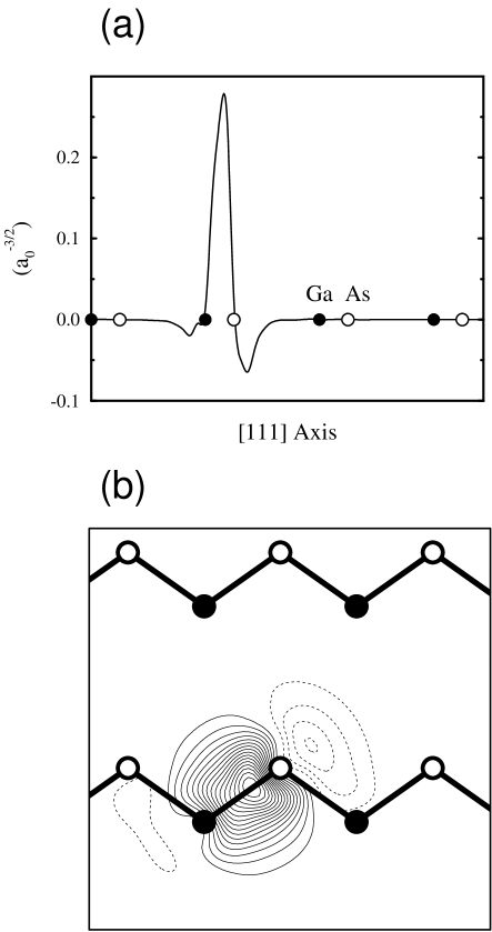
FIG. 2.: Maximally-localized Wannier function in GaAs, for the $8\times 8\times 8$ k-point sampling. (a) Profile along the Ga-As bond. (b) Contour plot in the (110) plane of the bond chains. The other Wannier functions lie on the other three tetrahedral bonds and are related by tetrahedral symmetries to the one shown.

In Fig. 2, we present plots showing one of these maximally-localized Wannier functions in GaAs, for the $8\times 8\times 8$ k-point sampling. Again, at the minimum $\Omega$, all four Wannier functions have become identical (under the symmetry operations of the tetrahedral group), and they are real, except for an overall complex phase. The shape of the Wannier functions is again that of $sp^{3}$ hybrids combining to form $\sigma$-bond orbitals; inversion symmetry is now lost, but the overall shape is otherwise closely similar to what was found in Si. The Wannier centers are still found along the bonds, but they have moved towards the As, at a position that is 0.617 times the Ga-As bond distance. It should be noted that these Wannier functions are also very similar to the localized orbitals that are found in linear-scaling approaches,[54] where orthonormality, although not imposed, becomes exactly enforced in the limit of an increasingly large localization region. This example highlights the connections between the two approaches. The characterization of the maximally-localized Wannier functions indicates the typical localization of the orbitals that can be expected in the linear-scaling approach. Moreover, such information ought to be extremely valuable in constructing an intelligent initial guess at the solution of the electronic structure problem in the case of complex or disordered systems.

TABLE III.: Localization functional $\Omega$ and its decomposition in invariant, off-diagonal, and diagonal parts, for the case of GaAs (units are Ų). The bottom valence band, the top three valence bands, and all four bands are separately included in the minimization. The star (^⋆) refers to the case in which the minimization is not actually performed, and the solution for the 1-band and 3-band cases is used. Sampling is performed with a $8\times 8\times 8$ mesh of k-points.

k set	$\Omega$	$\Omega_{\rm I}$	$\Omega_{\rm OD}$	$\Omega_{\rm D}$
1 band	$1.968$	$1.944$	$0$	$0.0238$
3 bands	$10.428$	$9.844$	$0.560$	$0.0245$
4 bands⋆	$12.396$	$8.038$	$4.309$	$0.0483$
4 bands	$8.599$	$8.038$	$0.555$	$0.0059$

As pointed out before, in GaAs we can have different choices for the Hilbert spaces that can be considered, so we also studied the case in which only the bottom band, or the top three, are used as an input for the the minimization procedure. Table III shows the spread functional and its various contributions for these different choices, where the bottom band is first treated as isolated; next the three $p$ bands are treated as a separate group; then these two solutions are used to construct a four-band solution, without further minimization; and finally, this is compared with the full four-band minimization. In composing the results for the 1-band and 3-band cases, we take the $1\times 1$ and $3\times 3$ unitary matrices that would give the minimum solution for the 1- and 3-band cases, and build from them a set of $4\times 4$ block-diagonal unitary matrices. The 4-band $\Omega$ that is obtained is exactly the sum of the two initial $\Omega$’s. Nevertheless, the bookkeeping changes: $\Omega_{\rm I}$ is reduced, with an equal and opposite contribution reappearing in $\Omega_{\rm OD}$. (The $\Omega_{\rm D}$’s sum up exactly, as they must.) If we then minimize this (saddle-point) solution, we recover the 4-band minimum: the invariant part (obviously) does not change, while $\Omega_{\rm D}$ increases to permit a larger reduction in $\Omega_{\rm OD}$, in correspondence to an increased interband mixing.

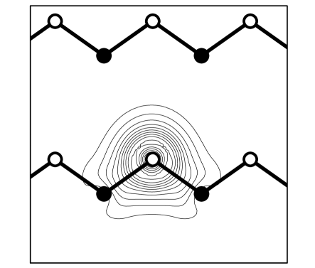
FIG. 3.: Contour plot, in (110) plane, of the maximally-localized Wannier function in GaAs for the $8\times 8\times 8$ k-point sampling when only the bottom valence band is considered.

In Fig. 3, we show the contour plot for the maximally-localized one-band Wannier function in GaAs, for the $8\times 8\times 8$ k-point sampling. The function is again real, and it shows the typical characteristics of an $s$ orbital centered around the anion; the tetrahedral symmetry of the lattice deforms the spherical orbital, introducing contributions that point along the two bond-chains (one in the (110) plane plotted, and one perpendicular to that plane). In the three-band case, on the other hand, the Wannier functions resemble three orthogonal atomic $p$ orbitals. It should be stressed that only when all the four bands are treated simultaneously do we achieve the overall maximum localization. This reinforces the picture in which the maximally localized orbitals correspond to the most natural “chemical bonds” in the system.

C Molecular C₂H₄

We have also studied the case of the ethylene molecule (C₂H₄), in order to make the connection with some standard chemistry concepts, and to highlight the relation of our formalism (derived from a k-space representation of extended Bloch orbitals) to the case of an isolated system as discussed in Sec. IV C 4. First of all, the molecule is modeled in periodic boundary conditions, in a supercell that is large enough to make the interaction with the periodic images negligible. Consequently, the band dispersion becomes also negligible, and $\Gamma$ sampling is all that is needed for total energies, forces, and densities. However, the spread functional is expected to converge slightly slower with k-point sampling, as discussed in Sec. IV C 4. We thus tested several k-point meshes. For the single k-point case, the mesh in reciprocal space is that formed by the $\Gamma$ point and all its periodical images, i.e., the reciprocal lattice vectors; our formalism remains equally applicable to such a case. One should bear in mind that if the supercell is not cubic, appropriate weight factors have to be added in the calculation of the derivatives (see Appendix B).

TABLE IV.: Coordinates (in Å) of the atoms and of the 6 Wannier centers in the ethylene molecule.

Species	$x$	$y$	$z$
H	$-1.235$	$0.936$	$0.000$
H	$1.235$	$-0.936$	$0.000$
H	$1.235$	$0.936$	$0.000$
H	$-1.235$	$-0.936$	$0.000$
C	$0.660$	$0.000$	$0.000$
C	$-0.660$	$0.000$	$0.000$
WF	$\overline{r}_{x}$	$\overline{r}_{y}$	$\overline{r}_{z}$
1	$-1.049$	$0.622$	$0.000$
2	$1.049$	$-0.622$	$0.000$
3	$1.049$	$0.622$	$0.000$
4	$-1.049$	$-0.622$	$0.000$
5	$0.000$	$0.000$	$0.327$
6	$0.000$	$0.000$	$-0.327$

We show in Table IV the coordinates for the C and H atoms at the structural minimum, together with the Wannier centers. We have used the local-density approximation for the exchange-correlation functional.[55] In this molecule, there are six occupied valence eigenstates, the lowest five being of C–H or C–C $\sigma$-bonding character, and the top (frontier) orbital being of C–C $\pi$-bonding character. If we treat the lowest five bonds as a composite group, we find as expected that the minimization of $\Omega$ leads to $\sigma$-bond-orbitals located on each of the C–H or C–C bonds. However, treating all six bands together, we find that the C–C $\pi$-bonding orbital mixes strongly with the C–C $\sigma$-bonding orbital to give two Wannier functions that are symmetrically disposed above and below the $x-y$ plane. Contour plots for the resulting C–H and C=C Wannier functions are shown in Fig. 4, and the locations of the Wannier centers are reported in Table IV. The picture that emerges from this “natural” symmetry breaking of the planar geometry is just the Lewis picture of the C=C double bond.

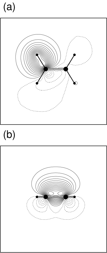
FIG. 4.: Contour plots for the maximally-localized Wannier functions in ethylene, C₂H₄. (a) One of the four C–H Wannier functions, shown in the $x-y$ plane. (b) One of the two C=C Wannier functions, shown in $x-z$ plane.

TABLE V.: The functional $\Omega$ and its decomposition, with increasing k-point sampling, for ethylene (units are Ų).

k set	$\Omega$	$\Omega_{\rm I}$	$\Omega_{\rm OD}$	$\Omega_{\rm D}$
$1\times 1\times 1$	$4.041$	$3.657$	$0.384$	$0$
$2\times 2\times 2$	$4.503$	$4.124$	$0.380$	$6\times 10^{-7}$
$3\times 3\times 3$	$4.600$	$4.222$	$0.377$	$3\times 10^{-7}$

In our calculations we have used a cubic supercell of side 7 $\AA$; this gives to each band a dispersion that is always smaller than 0.02 eV, and that originates from the interaction with the superperiodic images. Increasing the k-point sampling has negligible effects on the equilibrium positions of the C and H atoms and on the location of the Wannier centers. But it does still affect the localization functional, which displays a slower convergence with respect to the number of k-points used (although much faster than was the case for Si or GaAs). The results are summarized in Table V, where we show the $\Omega$ contributions for the maximally-localized Wannier functions with increasing k-point sampling. It is readily seen that the slow convergence is coming mostly from the invariant part of the functional; a finer k-point mesh provides both a more detailed sampling of the Brillouin Zone and a more accurate calculation of the gradients.

D LiCl

It is also interesting to look at a more ionic system, to understand the effect of electronegativity and band gap on the location and localization of the Wannier functions. We have studied rocksalt LiCl, treating all four valence bands (roughly Cl 3$s$ and 3$p$) as a unit, and again using an $8\times 8\times 8$ k-point sampling.

One could expect the Wannier functions to localize much more strongly around the anion than was the case for GaAs, and indeed this is what we find. However, we also find that the Wannier functions can reduce $\Omega$ further by mixing to form $sp^{3}$ hybrids, sitting on the vertices of a tetrahedron centered around the Cl atom, with each center at a distance of 0.449 Å from the Cl (the Li-Cl distance being 2.57 Å). We anticipated that these hybrids might prefer to align along the $\{111,\bar{1}\bar{1}1,\bar{1}1\bar{1},1\bar{1}\bar{1}\}$ or $\{11\bar{1},1\bar{1}1,\bar{1}11,\bar{1}\bar{1}\bar{1}\}$ sets of directions; if this were the case, the choice between the two sets (two degenerate global minima of $\Omega$) would constitute a kind of unphysical or “anomalous” symmetry breaking from cubic to tetrahedral. Instead, we find that $\Omega$ is, at least to our machine precision, rotationally invariant with respect to the orientation of the $sp^{3}$ hybrids, just as would be the case for an isolated Cl^- ion in free space. This implies that the tetrahedron of the Wannier centers around each Cl atom is free to rotate without any discernible decrease of localization.

Finally, consistent with the idea that a larger gap is linked to a higher degree of localization, we find a total $\Omega$=4.159 Ų, with $\Omega_{\rm I}$=3.354, $\Omega_{\rm OD}$=0.805 and $\Omega_{\rm D}$=1.2$\times$10^-5 Ų.

VII Discussion

We have discussed a technique for obtaining a set of well-localized Wannier functions for a given band or composite set of bands in a crystalline solid. We have in mind several kinds of applications for this method.

First, we believe that this approach may help to obtain chemical intuition about the nature of chemical bonds in solids, and to characterize trends in bonding properties within classes of solids. As emphasized in the introduction, the Wannier functions defined here are the natural generalization of the concept of “localized molecular orbitals” [20, 21, 22, 23, 24, 25] to the case of solids. As illustrated in the examples of GaAs and ethylene (C₂H₄) above, the determination of the Wannier functions can give chemical intuition into the nature of the bond orbitals of the material, including the spontaneous symmetry breaking that occurs in the Lewis picture of a double or triple bond. We also suspect that it may be instructive to generate, characterize and plot the Wannier functions across a series of compounds, e.g., for II-VI semiconductors as one varies from wide- to narrow-gap members, or in cubic perovskites of varying composition. Moreover, as emphasized by Hierse and Stechel,[10] the Wannier functions may be transferable to a considerable degree for similar bonds in different chemical systems (for example, for C-H or C-C bonds in a variety of hydrocarbons). It should be noted, however, that this is even more likely to be true for non-orthogonal Wannier-like functions,[10] as opposed to the orthogonal ones studied here.

Second, it is possible that the Wannier functions may prove suitable as a basis for use in constructing theories of interacting or strongly-correlated electron systems. For example, it might be possible to build good approximate correlated wavefunctions from sums of Slater determinants of the Wannier functions. For this purpose, one would clearly need to choose a set of bands that includes some low-lying unoccupied states of the one-particle mean-field Hamiltonian. Similarly, it might be possible to build accurate model Hamiltonians for for magnetic systems, or for transport properties of metals. (Again, for metals it would appear necessary to choose a composite group of bands that brackets the Fermi level, and to specify the occupation as a kind of density matrix in the Wannier indices.)

Third, the present scheme might prove useful for predicting the suitability of linear-scaling methods for different kinds of insulating materials. Since the linear-scaling methods [5] depend strongly on the localization properties of the Wannier functions (or, closely related, the density matrix), the present scheme might be a simple and useful way to characterize the degree of localization for a given target material. This information might then help predict whether the material is a good candidate for a linear-scaling method; and if so, what type of linear-scaling method is likely to work best, and what real-space cutoff parameter is likely to be required.

Finally, an important feature of the present approach is that it generates a list of the locations of the Wannier centers. This information alone can often be of crucial importance. In fact, we envisage a number of interesting applications in which one essentially throws away all other information about the Wannier functions, keeping only their locations. For example, the shift of the Wannier center away from the bond center might serve as a kind of measure of bond ionicity. Also, the vector sum of the Wannier centers immediately gives the bulk electronic polarization $\bf P$; all three Cartesian components of $\bf P$ can thus be determined simultaneously using a conventional k-mesh, instead of constructing separate special k-point strings to compute each separate Cartesian component of $\bf P$ as is needed otherwise.[14]

But more importantly, the information on the locations of the Wannier functions may open the possibility of calculating properties that cannot otherwise be obtained, especially for distorted, defective, or disordered systems. For example, it becomes possible not only to calculate the Born (dynamical) effective charge $Z^{*}$, but also to decompose it into displacements of individual neighboring Wannier centers. To illustrate this idea, we have carried out a calculation on a cubic supercell of GaAs containing 64 atoms ($\Gamma$-only k-point sampling), in which all atoms are in their equilibrium positions except for one Ga atom that is displaced by 0.1 Å along the $[111]$ direction. Observing the consequent displacement of the Wannier centers from their bulk crystalline positions, we find a total $Z_{\rm Ga}^{*}$ of 2.04, in good agreement with the established theoretical value of 1.99 as calculated by linear-response methods.[59] Moreover, in arriving at the total electronic $Z_{\rm Ga}^{*,\rm el}$=-0.96, we find contributions of -1.91, +0.65, and +0.30 from the groups of four first-neighbor, 12 second-neighbor, and remaining further-neighbor Wannier centers, respectively. It is interesting to note that inclusion of nearest-neighbor contributions alone would thus significantly overestimate the magnitude of $Z_{\rm Ga}^{*,\rm el}$, and that the second-neighbor Wannier centers move in the opposite direction to the Ga atom motion. If we repeat the calculation displacing one As atom, we obtain a total $Z_{\rm As}^{*}$ of -2.07 (the acoustic sum rule[60] is only approximately satisfied with a finite k-point sampling). The total electronic $Z_{\rm As}^{*,\rm el}$=-7.07 has now contributions of -1.74, -4.63, and -0.71 from the groups of four first-neighbor, 12 second-neighbor, and remaining further-neighbor Wannier centers, respectively.

In fact, the pattern of displacements of the Wannier centers can be regarded as defining a kind of coarse-grained representation of the polarization field, $\bf P(r)$. To illustrate this idea more directly, we have carried out a calculation for bulk GaAs in which a long-wavelength transverse optical (TO) phonon has been frozen in. We take the wavevector ${\bf q}=(\pi/4a)(\hat{x}+\hat{y})$ ($a$ is the lattice parameter) and relative displacements $\xi({\bf r})=\xi_{0}\sin({\bf q\cdot r})\hat{z}$ in a 16-atom supercell, composed of 8 unit cells repeated in the (110) direction. We assign a displacement amplitude $\xi_{0}=0.01a$ to the Ga sublattice, and $-\xi_{0}$ $M_{\rm Ga}/M_{\rm As}$ to the As sublattice ($M_{\rm Ga}$ and $M_{\rm As}$ are the masses of the two species; the center of mass doesn’t move). Observing the resulting displacements of the Wannier centers, we can obtain a picture on how the local polarization changes from cell to cell (say, by summing all the 4 Wannier centers surrounding one As atom); fitting these to the same form ${\bf P(r)}=P_{0}\sin({\bf q\cdot r})\hat{z}$, we obtain a $P_{0}$=0.249, and, via the acoustic sum rule ($Z_{\rm Ga}^{*,\rm el}+Z_{\rm As}^{*,\rm el}=-8$), we get $Z_{\rm Ga}^{*,\rm el}=-1.52$ and $Z_{\rm As}^{*,\rm el}=-6.48$. These results are only in fair agreement with the bulk values; the discrepancies might be due to the finite size of our supercell, or to not having used the proper eigenvector for the phonon mode considered. However, the main point of this demonstration is that, given the calculation on the supercell containing the frozen TO phonon, there is no other way that the transverse component of the polarization field could have been obtained. Since the mode is transverse, $\bf P(r)$ cannot be determined from the charge density; since ${\bf q}\neq{\bf 0}$, the Berry-phase approach does not apply; and since the displacement is finite, the linear-response approach is not directly applicable. However, the present scheme allows a direct finite-difference calculation of the transverse polarization field, a quantity that was previously unavailable.

It would be interesting to apply this kind of analysis to supercell simulations of amorphous systems such as $a$-H₂O or $a$-GaAs. Once again, while only the longitudinal part of $\bf P(r)$ can be determined from the charge density, a similar determination of both the longitudinal and transverse components is possible with access to the displacements of the Wannier centers, thus leading to a more complete theory of the dielectric properties of such systems. This information might be used to assist the approach of Ref. [43], in which the infrared absorption spectrum of an amorphous system is extracted from a molecular-dynamics simulation. As a limited test, we have carried out calculations for a 64-atom supercell of crystalline Si with random displacements typical of $\sim$1000K, and find that the calculation of the displaced Wannier centers is straightforward.

Finally, we conclude by pointing out that our work opens numerous possibilities for further development and future study. On a practical level, it might be useful to explore the use of more accurate, higher-order finite difference formulas for $\nabla_{\bf k}$ (see Appendix B) to see whether convergence with respect to k-point sampling can be improved. It might be interesting to apply our analysis within the semi-empirical tight-binding context, although it should be noted that matrix elements of $x$, $y$, and $z$ (and, for $\Omega_{\rm I}$, also of $r^{2}$) would be needed, in addition to the Hamiltonian and overlap matrix elements. Going beyond the scope of the present work, it might be interesting to other explore localization criteria e.g., the maximization of the Coulomb self-interaction of the Wannier functions. It would also be of great interest to develop a corresponding theory of maximally-localized non-orthogonal Wannier-like functions. (While the direct connection to the polarization properties would be lost, there would be important implications for some linear-scaling algorithms.) Finally, there are many questions of a mathematical character that deserve further study. For example, is it possible to prove that our Wannier functions (those that minimize $\Omega$) have exponential decay, even in the general non-centrosymmetric multi-band case? Are they always real, as conjectured in Sec. V B? And are there further results that can be derived regarding the interrelations between the metric tensor, the Berry connection, and the Berry curvature, as discussed in Appendix C? We hope that our work will stimulate some investigations of these questions.

A Minimization of spread functional in real space

In Sec. III above, the problem of finding the optimally localized Wannier functions for a periodic system was formulated directly in real space. In this Appendix, we briefly reformulate the problem for the case of a finite system (cluster, molecule, etc.), and sketch how the minimization of the functional can be performed in this case. This provides a complementary perspective to the k-space procedure discussed in the main text.

We change notation $|{\bf R}n\rangle\rightarrow|i\rangle$ and now refer to the $i$ as “localized orbitals” rather than “Wannier functions,” but their meaning is the same: they are a set of orthonormal orbitals spanning the Hamiltonian eigenstates in an energy range of interest (e.g., for the occupied valence states of a molecule or cluster).

Following the approach of Sec. III, we decompose $\Omega=\sum_{i}[\langle r^{2}\rangle_{i}-\bar{\bf r}_{i}^{2}]$ into an invariant part $\Omega_{\rm I}=\sum_{\alpha}{\rm tr}\,[Pr_{\alpha}Qr_{\alpha}]$ (where $P=\sum_{i}|i\rangle\langle i|$ and $Q=1-P$) and a remainder $\widetilde{\Omega}=\sum_{\alpha}\sum_{i\neq j}\,|\langle i|r_{\alpha}|j\rangle|^{2}$. Defining matrices $X_{ij}=\langle i|x|j\rangle$, $X_{{\rm D},ij}=X_{ij}\,\delta_{ij}$, $X^{\prime}=X-X_{\rm D}$, and similarly for $Y$ and $Z$, this can be rewritten

$$\widetilde{\Omega}={\rm tr}\,[X^{\prime 2}+Y^{\prime 2}+Z^{\prime 2}]\;\;.$$ (A1)

Thus if $X$, $Y$, and $Z$ could be simultaneously diagonalized, then $\widetilde{\Omega}$ could be minimized to zero, but for non-commuting matrices this is not possible. In a sense, our job is to perform the optimal approximate simultaneous co-diagonalization of the three Hermitian matrices $X$, $Y$, and $Z$ by a single unitary transformation. We are not aware of a formal solution for this problem, but a steepest-descent numerical solution is fairly straightforward. Since ${\rm tr}\,[X^{\prime}X_{\rm D}]=0$, etc.,

$$d\Omega=2\,{\rm tr}\,[X^{\prime}dX+Y^{\prime}dY+Z^{\prime}dZ]\;\;.$$ (A2)

We consider an infinitesimal unitary transformation $|i\rangle\;\rightarrow\;|i\rangle+\sum_{j}W_{ji}|j\rangle$ (where $dW$ is antihermitian), from which $dX=[X,dW]$, etc. Inserting in Eq. (A2) and using ${\rm tr}\,[A[B,C]]=\,{\rm tr}\,[C[A,B]]$ and $[X^{\prime},X]=[X^{\prime},X_{\rm D}]$, we obtain $d\Omega={\rm tr}\,[dW\,G]$ where

$$G=2\,\Bigl{\{}[X^{\prime},X_{\rm D}]+[Y^{\prime},Y_{\rm D}]+[Z^{\prime},Z_{\rm D}]\Bigr{\}}\;\;,$$ (A3)

so that the desired gradient is ${d\Omega/dW}=G$ as given above. The minimization can then be carried out using steepest descents following the general approach outlined in Sec. IV D. More sophisticated but related methods are discussed in Ref. [25].

If this approach is applied to a finite system having a crystalline interior, the solutions in the interior are expected to correspond precisely with the maximally-localized Wannier functions as determined using the k-space methods of the main text. In the vicinity of surfaces or defects, or for disordered materials, the solutions will essentially correspond to the “generalized Wannier functions” discussed by previous authors.[26, 48, 49, 50]

B Finite-difference formulas for k-space grids

We assume that the Brillouin zone has been discretized into a uniform Monkhorst-Pack mesh.[58] Let $\bf b$ be a vector connecting a k-point to one of its near neighbors, and let $Z$ be the number of such neighbors to be included in the finite-difference formulas. We seek the simplest possible finite-difference formula for $\nabla_{\bf k}$, i.e., the one involving the smallest possible $Z$. When the Bravais lattice point group is cubic, it will only be necessary to include the first shell of $Z=6$, 8, or 12 k-neighbors for simple cubic, bcc, or fcc k-space meshes, respectively. Otherwise, further shells must be included until it is possible to satisfy the condition

$$\sum_{\bf b}w_{b}\,b_{\alpha}b_{\beta}=\delta_{\alpha\beta}$$ (B1)

by an appropriate choice of a weight $w_{b}$ associated with each shell $|{\bf b}|=b$. For the three kinds of cubic mesh, Eq. (B1) is satisfied with $w_{b}=3/Zb^{2}$ (single shell). Taking next the slightly more complicated case of an orthorhombic lattice, one can let $\bf b$ run over the two nearest neighbors in each Cartesian direction ($Z=6$), with $w_{b}=1/2b_{x}^{2}$ for the two neighbors at $\pm b_{x}\hat{x}$, etc. Even in the worst case of minimal (triclinic) symmetry, only six pairs of neighbors ($Z=12$) should be needed, as the freedom to choose six weights should allow one to satisfy the six independent conditions comprising Eq. (B1).

Now, if $f(\bf k)$ is a smooth function of $\bf k$, its gradient can be expressed as

$$\nabla f({\bf k})=\sum_{\bf b}w_{b}\,{\bf b}\,[f({\bf k+b})-f({\bf k})]\;\;.$$ (B2)

We can check the correctness of this finite-difference formula by applying it to the case of a linear function $f({\bf k})=f_{0}+{\bf g\cdot k}$, for which we find $\nabla_{\alpha}f({\bf k})=\sum_{\bf b}w_{b}\sum_{\beta}b_{\alpha}g_{\beta}b_{\beta}=g_{\alpha}$. In a similar way,

$$|\nabla f({\bf k})|^{2}=\sum_{\bf b}w_{b}\,[f({\bf k+b})-f({\bf k})]^{2}\;\;.$$ (B3)

We note that improved accuracy and k-set convergence might be obtained by utilizing improved, higher-order finite-difference formulas involving more shells of neighboring k-points, but we have not explored this possibility here.

C Geometric properties and complexity of electron bands

Consider a manifold of $J$ orthonormal states $|\psi_{n}(\lambda)\rangle$, $n=1,...,J$, depending on a continuous $d$-dimensional parameter $\lambda$. Alternatively, one can view these as representing the projection $P(\lambda)=\sum_{n}|\psi_{n}(\lambda)\rangle\langle\psi_{n}(\lambda)|$. For the application to electron bands in crystals, we identify $\lambda\rightarrow\bf k$ and $\psi_{n}(\lambda)\rightarrow u_{n\bf k}$. Here, we investigate the geometric properties of such a manifold, generalizing the single-state ($J=1$) results of Refs. [34, 35, 36] to the multi-state case.

One can define two kinds of intrinsic geometric properties: a geometric distance and a geometric phase. We consider the former first. The geometric distance $D_{12}$ between two points $\lambda_{1}$ and $\lambda_{2}$ is here taken to be

$$D_{12}^{2}\,=\,{\rm tr}[P_{1}Q_{2}]\,=\,{\textstyle{1\over 2}}\,\|P_{1}-P_{2}\|^{2}\;\;,$$ (C1)

where $Q(\lambda)=1-P(\lambda)$. In the case of a single state, this becomes $D_{12}^{2}=1-|\langle\psi_{1}|\psi_{2}\rangle|^{2}$, which for small separations is consistent with the slightly different definition $D_{12}^{2}=2-2|\langle\psi_{1}|\psi_{2}\rangle|$ of Ref. [34]. Considering the distance for infinitesimal separations, one can define a Riemannian metric[34]

$$D_{\lambda,\lambda+d\lambda}^{2}\,=\sum_{\alpha\beta}\,g_{\alpha\beta}\,d\lambda_{\alpha}\,d\lambda_{\beta}\;\;.$$ (C2)

Introducing the notation $\psi_{n,\alpha}=d\psi_{n}/d\lambda_{\alpha}$, etc., and making use of

$$0=\langle\psi_{n}|\psi_{m,\alpha}\rangle+\langle\psi_{n,\alpha}|\psi_{m}\rangle\;\;,$$ (C3)

$$0=\langle\psi_{n}|\psi_{m,\alpha\beta}\rangle+\langle\psi_{n,\alpha\beta}|\psi_{m}\rangle+2\,{\rm Re}\,\langle\psi_{n,\alpha}|\psi_{m,\beta}\rangle\;\;,$$ (C4)

which follow from the fact that the $\psi_{n}$ remain orthonormal at first and second order in $d\lambda$, the metric $g_{\alpha\beta}$ becomes, after some manipulation,

$$g_{\alpha\beta}=\,{\rm Re}\,\sum_{n}\,\langle\psi_{n,\alpha}|\psi_{n,\beta}\rangle-\,\sum_{mn}\,\langle\psi_{n,\alpha}|\psi_{m}\rangle\,\langle\psi_{m}|\psi_{n,\beta}\rangle\;\;,$$ (C5)

which reduces in the single-band case to the expression of Pati.[34]

From Eq. (C1) it is obvious that the distance, and thus the metric, are gauge-invariant quantities. These are therefore intrinsic properties of the manifold. One way of thinking about the metric is to observe that for any given path in $\lambda$ space, the line integral of $g^{1/2}$ along the path provides a measure of the total “quantum distance” along the path; intuitively, it is a measure of the amount of change of character of the states as one traverses the path. The physical meaning of this distance for the case of temporal evolution of quantum states is discussed in Refs. [34, 35, 36].

The second type of geometric object that can be defined is a “geometric phase” or “Berry phase.”[37] Here, one is interested in considering closed paths in $\lambda$ space, and relating the phase (or, for the multi-state case, the unitary rotation) induced by adiabatic (“parallel”) transport along the path. The multi-state (“non-Abelian”) case has been discussed by Wilczek and Zee[38], Mead,[39] and Resta.[19] One can define a (non-gauge-invariant) Berry connection

$$A_{\alpha,nm}=i\,\langle\psi_{n}|\psi_{m,\alpha}\rangle$$ (C6)

and a (gauge-covariant) Berry curvature

$$B_{\alpha\beta}^{nm}=-\partial_{\alpha}A_{\beta,nm}+\partial_{\beta}A_{\alpha,nm}+i\,[A_{\alpha},A_{\beta}]_{nm}\;\;.$$ (C7)

The invariants of the latter, such as

$${\rm tr}\,B_{\alpha\beta}=2\,{\rm Im}\,\sum_{n}\,\langle\psi_{n,\alpha}|\psi_{n,\beta}\rangle\;\;,$$ (C8)

[see Eq. (3.29) of Ref. [19]] are thus gauge-invariant. (We shall use the notation ‘tr’ and ‘Tr’ to denote electronic and Cartesian traces, respectively.)

There is a tantalizing similarity between the metric $g_{\alpha\beta}$, Eq. (C5), and the quantum trace of the Berry curvature, Eq. (C8). In fact, defining the gauge-invariant quantity

$${\cal F}_{\alpha\beta}=\sum_{n}\,\langle\psi_{n,\alpha}|Q|\psi_{n,\beta}\rangle$$ (C9)

where again $Q=1-P$, and using Eq. (C3) to show that the second term in Eq. (C5) is intrinsically real, we obtain simply $g_{\alpha\beta}={\rm Re}\,{\cal F}_{\alpha\beta}$ and ${\rm tr}\,B_{\alpha\beta}=2\,{\rm Im}\,{\cal F}_{\alpha\beta}$. This suggests that there may be some deep connections between the two quantities.[34, 35, 36] In the case where the states $\psi_{n}$ are eigenstates of a Hamiltonian $H(\lambda)$, one moreover has[19]

$${\cal F}_{\alpha\beta}=\sum_{n=1}^{J}\,\sum_{m=J+1}^{\infty}\;{\langle\psi_{n}|H_{\alpha}|\psi_{m}\rangle\langle\psi_{m}|H_{\beta}|\psi_{n}\rangle\over(E_{n}-E_{m})^{2}}$$ (C10)

where $H_{\alpha}=dH(\lambda)/d\lambda_{\alpha}$.

We now return to the case of electron bands in crystals, $\lambda\rightarrow\bf k$ and $\psi_{n}(\lambda)\rightarrow u_{n\bf k}$, and discuss the geometric properties induced by the band projection operator $P^{\bf(k)}$. Note that $g$, $A$, and $B$ have units of $l^{2}$, $l$, and $l^{2}$, respectively. Again focusing first on the metric, and comparing Eq. (40) with the definitions (C1) and (C2), we find

$$\Omega_{\rm I}\,=\,{1\over N}\,\sum_{\bf k,b}\sum_{\alpha\beta}\,w_{b}\,g_{\alpha\beta}\,b_{\alpha}\,b_{\beta}$$ (C11)

or, using Eq. (B1) and restoring the continuum limit,

$$\Omega_{\rm I}\,=\,{V\over(2\pi)^{3}}\,\int_{\rm BZ}d{\bf k}\,{\rm Tr}\,g{(\bf k)}\;\;,$$ (C12)

where the integral is over the Brillouin zone. Thus, the invariant part of the spread functional is nothing other than the Brillouin-zone average of the trace of the metric!

It may be interesting to see whether other global properties of the metric might be given some physical interpretation. In particular, we define a dimensionless and gauge-invariant quantity

$$C=\int_{\rm BZ}d{\bf k}\;{\rm det}^{1/2}\,g({\bf k})\;\;.$$ (C13)

We shall call this the “complexity” of the bands. Mathematically, it is really nothing other than the volume of the Brillouin zone as measured according to the metric $g$. However, we have called it the “complexity” because it measures the variation of the character of the band projection operator $P^{(\bf k)}$ throughout the Brillouin zone. Everything said here applies to any isolated band or composite group of bands, but we have in mind primarily the case where all the occupied valence bands in an insulator are considered as a composite group. In this case, and assuming that one is only interested in quantities (such as total energies and forces) that can be expressed as a trace over the bands, the complexity might thus be expected to reflect (and even predict) the number of k-points needed for an accurate sampling of the Brillouin zone. We have not tested this idea numerically, but this would clearly be an interesting avenue for future exploration.

Turning now to phase properties, we note that a finite-different representation of the Berry connection is

$$A_{\alpha,mn}\,=\,i\,\sum_{b}\,w_{b}\,b_{\alpha}\left[\,M_{mn}^{\bf(k,b)}\,-\,\delta_{mn}\,\right]\;\;.$$ (C14)

Restoring the continuum limit in $k$-space, we can write

$$\bar{\bf r}_{n}\,=\,{V\over(2\pi)^{3}}\,\int_{\rm BZ}d{\bf k}\,{\bf A}_{nn}({\bf k})\;\;,$$ (C15)

and more generally,

$$\langle{\bf 0}m|{\bf r}|{\bf R}n\rangle\,=\,{V\over(2\pi)^{3}}\,\int_{\rm BZ}d{\bf k}\,{\bf A}_{mn}({\bf k})\,e^{i\bf k\cdot R}\;\;.$$ (C16)

The right-hand side is just ${\bf A}_{mn}({\bf R})$, the Fourier coefficient of the Berry curvature. Eq. (C15) is just the expression for the position of the Wannier center, which contributes to the electronic polarization.[3, 14, 16, 19] Moreover,

$$\widetilde{\Omega}_{\rm D}\,=\,\sum_{n}\,{V\over(2\pi)^{3}}\,\int_{\rm BZ}d{\bf k}\,\left|\,{\bf A}_{nn}({\bf k})\,-\,\bar{\bf r}_{n}\,\right|^{2}\;\;,$$ (C17)

$$\widetilde{\Omega}_{\rm OD}\,=\,\sum_{m\neq n}\,{V\over(2\pi)^{3}}\,\int_{\rm BZ}d{\bf k}\,\left|\,{\bf A}_{mn}({\bf k})\,\right|^{2}\;\;.$$ (C18)

Eqs. (C17-C18) show that the non-invariant parts of the spread functional are also conveniently written in terms of the Berry connection. If the above equations are reexpressed in terms of the Fourier coefficients $A_{mn}\bf(R)$, Eqs. (23) and (24) are immediately recovered.

In the single-band case, we showed in Sec. IV C 2 that the minimum value of $\widetilde{\Omega}$ could be related to the transverse part of the Berry connection, which in turn is determined by the gauge-invariant Berry curvature. In the multiband case, the Berry curvature $B_{\alpha\beta}^{mn}({\bf k})$ is no longer gauge-invariant, and it is not obvious whether it is possible to make a corresponding decomposition. Nevertheless, one can derive similar correspondences as those above for $\bf A$. So,

$$B_{\alpha\beta}^{mn}({\bf k})\,=\,-i\,\langle\,u_{m,\alpha}\,|\,Q\,|\,u_{n,\beta}\,\rangle\,+i\,\langle\,u_{m,\beta}\,|\,Q\,|\,u_{n,\alpha}\,\rangle\,\;\;,$$ (C19)

$$B_{\alpha\beta}^{mn}({\bf R})\,=\,-i\,\langle\,u_{m}\,|\,r_{\alpha}Qr_{\beta}\,-\,r_{\beta}Qr_{\alpha}\,|\,u_{n}\,\rangle\;\;.$$ (C20)

Making use of $r_{\alpha}Qr_{\beta}-r_{\beta}Qr_{\alpha}=[Pr_{\alpha}P,Pr_{\beta}P]$, one finds

$$\|\,[Pr_{\alpha}P,Pr_{\beta}P]\,\|_{\rm c}^{2}\, = \,\sum_{\bf R}\,\sum_{mn}\,|\,B_{\alpha\beta}^{mn}({\bf R})\,|^{2}$$ (C21)

$$= \,{V\over{(2\pi)^{3}}}\,\int_{\rm BZ}\,d{\bf k}\,\left\|\,B_{\alpha\beta}({\bf k})\,\right\|^{2}\;\;.$$ (C22)

Each form above is manifestly gauge-invariant and positive-definite. Thus, it can be seen that the Berry curvature will vanish if and only if the band-projected position operators $PxP$, $PyP$, and $PzP$ commute with one another; as discussed following Eq. (21), this is also just the condition that $\widetilde{\Omega}$ vanishes at the minimum.

REFERENCES

- [1] G.H. Wannier, Phys. Rev. 52, 191 (1937).
- [2] W. Kohn, Phys. Rev. 115, 809 (1959).
- [3] E.I. Blount, Solid State Physics 13, 305 (1962).
- [4] W. Kohn, Phys. Rev. B 7, 4388 (1973).
- [5] G. Galli, Curr. Opin. Sol. State Mater. Sci. 1, 864 (1996).
- [6] G. Galli and M. Parrinello, Phys. Rev. Lett. 69, 3547 (1992).
- [7] F. Mauri, G. Galli, and R. Car, Phys. Rev. B 47, 9973 (1993); F. Mauri and G. Galli, Phys. Rev. B 50, 4316 (1994).
- [8] P. Ordejón, D. Drabold, M.P. Grumbach, and R.M. Martin, Phys. Rev. B 48, 14646 (1993); Phys. Rev. B 51, 1456 (1995).
- [9] W. Kohn, Chem. Phys. Lett. 208, 167 (1993).
- [10] W. Hierse and E. B. Stechel, Phys. Rev. B 50, 1781 (1994).
- [11] J. Kim, F. Mauri and G. Galli, Phys. Rev. B 52, 1640 (1995).
- [12] E. Hernández and M.J. Gillan, Phys. Rev. B 51, 10157 (1995); E. Hernández, M. J. Gillan, and C.M. Goringe, Phys. Rev. B 53, 7147 (1996).
- [13] P. Ordejón, E. Artacho and J.M. Soler, Phys. Rev. B 53, R10441 (1996).
- [14] R.D. King-Smith and D. Vanderbilt, Phys. Rev. B 47, 1651 (1993).
- [15] D. Vanderbilt and R.D. King-Smith, Phys. Rev. B 48, 4442 (1993).
- [16] R. Resta, Rev. Mod. Phys. 66, 899 (1994).
- [17] G. Ortiz and R.M. Martin, Phys. Rev. B 49, 14202 (1994).
- [18] R.W. Nunes and D. Vanderbilt, Phys. Rev. B 50, 17611 (1994).
- [19] R. Resta, Berry Phase in Electronic Wavefunctions, Troisième Cycle Lecture Notes (Ecole Polytechnique Fédérale, Lausanne, Switzerland, 1996).
- [20] S.F. Boys, Rev. Mod. Phys. 32, 296 (1960).
- [21] J.M. Foster and S.F. Boys, Rev. Mod. Phys. 32, 300 (1960).
- [22] C. Edmiston and K. Ruedenberg, Rev. Mod. Phys. 35, 457 (1963).
- [23] S.F. Boys, in Quantum Theory of Atoms, Molecules, and the Solid State, P.-O. Löwdin, ed. (Academic Press, New York, 1966), p. 253.
- [24] H. Weinstein, R. Pauncz, and M. Cohen, Adv. At. Mol. Phys. 7, 97 (1971).
- [25] J.M. Leonard and W.L. Luken, Theoret. Chim. Acta 62, 107 (1982); Int. J. Quant. Chem. 25, 355 (1984).
- [26] W. Kohn and J. Onffroy, Phys. Rev. B 8, 2485 (1973).
- [27] P.W. Anderson, Phys. Rev. Lett. 21, 13 (1968).
- [28] D. Bullett, in Solid State Physics: Advances in Research and Applications, edited by H. Ehrenreich and D. Turnbull (New York, Academic, 1980), p. 129.
- [29] W.M.C. Foulkes and D.M. Edwards, J. Phys. Cond. Matt. 5, 7987 (1993).
- [30] We find empirically that the maximally localized Wannier functions are always real, once the arbitrary overall phase is removed. This observation is discussed and justified in Sec. V B.
- [31] S. Kivelson, Phys. Rev. B 26, 4269 (1982).
- [32] Q. Niu, Mod. Phys. Lett. B 5, 923 (1991).
- [33] A. Nenciu and G. Nenciu, J. Phys. A 15, 3313 (1982); G. Nenciu, Rev. Mod. Phys. 63, 91 (1991).
- [34] A.K. Pati, Physics Letters A 159, 105 (1991).
- [35] J. Anandan and Y. Aharonov, Phys. Rev. Lett. 65, 1697 (1990).
- [36] A.K. Pati and A. Joshi, Phys. Rev. A 47, 98 (1993).
- [37] M. V. Berry, Proc. R. Soc. Lond. A 392, 45 (1984).
- [38] F. Wilczek and A. Zee, Phys. Rev. Lett. 52, 2111 (1984).
- [39] C.A. Mead, Rev. Mod. Phys. 64, 51 (1992).
- [40] M.-C. Chang and Q. Niu, Phys. Rev. B 53, 7010 (1996).
- [41] G. Weinreich, Solids: Elementary Theory for Advanced Students (Wiley, New York, 1965), Ch. 8.
- [42] This discussion also applies to the k-point sampling in the surface-normal direction for periodic slab supercell calculations.
- [43] A. Debernardi, M. Bernasconi, M. Cardona and M. Parrinello, submitted to Appl. Phys. Lett; P.L. Silvestrelli, M. Bernasconi and M. Parrinello, submitted to Chem. Phys. Lett.
- [44] S. Satpathy and Z. Pawlowska, Phys. Stat. Sol. (b) 145, 555 (1988).
- [45] G. Nenciu, Commun. Math. Phys. 91, 81 (1983).
- [46] J. des Cloizeaux, Phys. Rev. 135, A685 (1964).
- [47] J. des Cloizeaux, Phys. Rev. 135, A698 (1964).
- [48] J.J. Rehr and W. Kohn, Phys. Rev. B 10, 448 (1974).
- [49] M.R. Geller and W. Kohn, Phys. Rev. B 48, 14085 (1993).
- [50] A. Nenciu and G. Nenciu, Phys. Rev. B 47, 10112 (1993).
- [51] E.O. Kane and A.B. Kane, Phys. Rev. B 17, 2691 (1978).
- [52] C. Tejedor and J.A. Verges, Phys. Rev. B 19, 2283 (1979).
- [53] M.R. Pederson and C.C. Lin, Phys. Ref. B 35, 2273 (1987).
- [54] P. Fernández, A. Dal Corso, F. Mauri, and A. Baldereschi, Phys. Rev. B 55, R1909 (1997).
- [55] See, e.g., R. O. Jones and O. Gunnarsson, Rev. Mod. Phys. 61, 689 (1989).
- [56] M. C. Payne, M. P. Teter, D. C. Allan, T. A. Arias, and J. D. Joannopoulos, Rev. Mod. Phys. 64, 1045 (1992); D. Vanderbilt, Phys. Rev. B 41, 7892 (1990).
- [57] J. S. Lin, A. Qteish, M. C. Payne, and V. Heine, Phys. Rev. B 47, 4174 (1993).
- [58] H.J. Monkhorst and J.D. Pack, Phys. Rev. B 13, 5188 (1976).
- [59] S. de Gironcoli, S. Baroni, and R. Resta, Phys. Rev. Lett. 62, 2853 (1989).
- [60] R. Pick, M. H. Cohen and R. M. Martin, Phys. Rev. B 1, 910 (1970).