Eu-Eu exchange interaction and Eu distribution in Pb_1-xEu_xTe from magnetization steps

Abstract

The magnetization of Pb_1-xEu_xTe samples with $x$ = 1.9, 2.6 and 6.0% was measured at 20 mK in fields up to 50 kOe, and at 0.6 K in fields up to 180 kOe. The 20 mK data show the magnetization steps (MSTs) arising from pairs and from triplets. The pair MSTs are used to obtain the dominant Eu-Eu antiferromagnetic exchange constant, $J/k_{B}=-0.264\pm 0.018$ K. The exchange constant for triplets is the same. Comparison of the magnetization curves with theoretical simulations indicates that the Eu ions are not randomly distributed over all the cation sites. The deviation from a random distribution is much smaller if $J$ is assumed to be the nearest-neighbor exchange constant $J_{1}$ rather than the next-nearest-neighbor exchange constant $J_{2}$. On this basis, $J$ is tentatively identified as $J_{1}$. However, the possibility that $J=J_{2}$ cannot be excluded completely. To obtain agreement with the data, it must be assumed that the Eu ions tend to bunch together. Comparision with microprobe data indicates that the length scale for these concentration variations is smaller than a few $\mu$m. The theoretical simulations in the present work improve on those performed earlier by including clusters larger than three spins.

I INTRODUCTION

An important group of dilute magnetic semiconductors (DMS) are lead salts in which a fraction of the Pb ions have been replaced by Eu ions.[1] Pb_1-xEu_xTe is one member of this group. The other members are Pb_1-xEu_xSe and Pb_1-xEu_xS. All these materials have the rock-salt structure, with an fcc cation lattice. The Eu²⁺ ion, with 7 electrons in the half-filled 4$f$ shell, has zero orbital angular momentum and total spin S=7/2. EPR data show that in Pb_1-xEu_xTe $g=1.98$ and that the spin hamiltonian for the Eu²⁺ ion contains a very small crystal-field anisotropy.[2]

It has been known for several years that the Eu–Eu exchange interaction in these IV–VI DMS is two orders of magnitude smaller than the Mn–Mn exchange interaction in the traditional II–VI DMS (e.g., Cd_1-xMn_xTe). In both types of DMS the exchange interaction is antiferromagnetic (AF), but the leading Eu–Eu exchange constant $J$ is of order $-0.1$ K, compared to $-10$ K for the Mn–Mn exchange constant.

Much of the early information concerning these Eu–Eu exchange interactions came from measurements of the Curie-Weiss temperature $\theta$, and from analysis of high-field magnetization data at $T=4.2$ K.[3, 4, 5] As discussed later, both of these methods yield only a rough estimate of the dominant AF exchange constant $J$. In the present paper we present an accurate determination of $J$ in Pb_1-xEu_xTe using the magnetization-steps (MSTs) method.[6, 7] Because $|J|$ is of order 0.1 K, the observation of the MSTs required the use of a dilution refrigerator operating well below 0.1 K.

In addition to yielding $J$, the low-temperature magnetization data also gave information about the distribution of the Eu ions over the cation sites . Such information is not readily available by other means. The analysis indicates that the distribution is not perfectly random (equal probability of occupation of all cation sites in the crystal). Instead, the Eu ions tend to bunch together. Another important issue is whether the dominant AF exchange constant $J$ corresponds to the nearest-neighbor (NN) or to the next-nearest-neighbor (NNN) exchange constant, $J_{1}$ or $J_{2}$ , respectively. This issue is addressed on the basis of the results for the Eu spatial distribution.

II THEORY

Much of the relevant theory was discussed in a recent paper on the MSTs in Pb_1-xEu_xSe.[8] We refer the reader to this earlier paper, and confine ourselves here to a summary of the main points. Some newer theoretical results are also mentioned.

As a first approximation we consider a simple model which captures the main features of the experimental data. In this “single-$J$” model for a DMS, only one AF exchange constant $J$ is included. Other exchange constants, and all anisotropies, are neglected. In this model each Eu ion on the fcc sublattice belongs to a particular type of “cluster”. The cluster types considered explicitly in Ref. [8] are: singles (isolated magnetic ions which are not connected by any exchange bonds), pairs, open triplets (OTs), and closed triplets (CTs). More recently the six types of quartets in the fcc lattice were considered also.[9]

Assuming that $J$ is negative (antiferromagnetic), the magnetization curve at low $T$ ($k_{B}T<<|J|$) for clusters of a given type has two main features: a quick saturation of the zero-field moment followed by a series of MST’s. [8, 9] This behavior is illustrated by the exact calculation of the magnetization curve for small clusters in this simple model. We will use normalized fields $h_{n}=g\mu_{B}H_{n}/|J|$ for the step positions. Pairs of Eu²⁺ ions ($S=7/2$) have no zero-field moment. The seven MSTs from pairs occur at normalized fields $h_{n}=2,4,...14$. Thus the pairs saturate at $g\mu_{B}H=14|J|$. The next most important clusters are open triplets. They have a zero-field groundstate with a net spin of 7/2 which saturates quickly. The MSTs occur at $h_{n}=9,11...21$. Closed triplets have their MSTs at $h_{n}=1,3...21$. Note that the last three MSTs due to triplets occur when the pairs are already saturated. For five of the six types of quartets the series of MSTs end at 28$|J|$; only the “string quartet” ramp ends at a lower field $g\mu_{B}H=24.2|J|$.[9]

The exchange constant $J$ is usually obtained from the observed $H_{n}$ for pairs since, except for singles, these are the most numerous. As was done in Ref. [8], we estimate an uncertainty in the determination of $J$ due to simplifications introduced by the single-$J$ model. The cubic crystal-field anisotropy, the dipole-dipole interaction, and exchange constants other than $J$ basically shift and broaden the MSTs. Their effects on the positions of the MSTs from pairs are included in the equation

$$g\mu_{B}H_{n}=2n|J|+\Delta_{n}$$ (1)

with $n=1,2...7$. The shifts $\Delta_{n}$ depend on $n$, the orientation of the sample (anisotropy) and the concentration (further neighbor exchange constants). We have calculated the magnetization and step postition of pairs taking into account the cubic crystal field and dipole-dipole interactions, using known parameters.[2] If $J$ is determined from a fit to Eq. (1), assuming a constant $\Delta_{n}$ (the procedure used below), the resulting error due to the crystal field anisotropy is less than 5%. The error due to dipole-dipole interactions is less than 1%.

Exchange interactions with further neighbors (not included in the single-$J$ model will also shift and broaden the MSTs.[10] These effects will be discussed later in connection with the data analysis.

The magnetization $M$ of the sample as a whole is obtained by adding the contributions of the various cluster types. The contribution of each cluster type is the product of the magnetization per cluster and the number of clusters of that type. To calculate the number of clusters of a given type one needs to know how the magnetic ions are distributed over the cation sites. Normally, a random distribution is assumed. The populations of the various cluster types are then well known.[9, 11] As discussed later, deviations from a random distribution can be detected by analyzing the measured magnetization curve at low temperatures. The ability to detect such deviations is a major advantage. Any tendency of the magnetic ions to bunch together or to avoid each other is revealed. The determination of the AF exchange constant $J$ is independent of the spatial distribution however.

In Ref. [8] the theoretical simulations of the magnetization curves included clusters up to triplets. In the present work the simulations were improved by adding the contributions of the six types of quartets.[9] In addition a rough estimate of the contribution of clusters larger than quartets was also included, as will be discussed shortly, so that all the spins were accounted for.

Clusters larger than quartets (quintets, sextets, etc.) will be referred to collectively as “others”. If the zero-field ground state of any such cluster has a net spin then this net spin will align rapidly with $H$ at low $T$. At higher fields a series of MSTs will occur. In practice, the MSTs from large clusters are very small in size, so that they are not resolved. The series of MSTs from a given cluster type then merges to form a ramp. The ramp ends at a field which depends on the cluster type.

The magnetization curve of the others is therefore a sum of many initial fast rises of $M$ followed by a superposition of many ramps ending at different fields. Here, we use an approximation in which the contribution of the others is represented by a single initial fast rise of $M$ followed by one ramp. The initial fast rise is approximated by a Brillouin function for spin 7/2 with a saturation value corresponding to 1/5 of the saturation value of the others. The 1/5 weight is motivated by earlier results for the initial rise of the magnetization.[6] The remaining magnetization rise (4/5 of the saturation value of the others) is approximated by a single ramp which starts at $H=0$ and ends at $g\mu_{B}H=35|J|$. The latter value is expected to be slightly higher than the average saturation value for all quintets but lower than the average saturation value of sextets.

For our samples, the contribution of others to the magnetization was small, only 0.2% of the saturation magnetization $M_{0}$ for $x=1.9\%$, and only 0.6% of $M_{0}$ for $x=2.6\%$. Even for the sample with $x=6\%$ the others contributed only 9% of $M_{0}$. Our approximation for the contribution of the others should therefore be adequate.

III EXPERIMENTAL TECHNIQUES

The three Pb_1-xEu_xTe samples were grown by the Bridgman method. The Eu concentration $x$ was determined from the saturation magnetization. A moment of $6.93\mu_{B}$ per Eu ion (based on $S=7/2$ and $g=1.98$) was assumed. A small correction for the lattice susceptibility, $\chi_{d}=-3\times 10^{-7}$ emu/g, was applied.[3] The results for the three samples gave $x$ = 1.9, 2.6 and 6.0%. These values are supported by the Curie constants, obtained from susceptibility data, which gave $x$ = 1.9, 2.4, and 5.9%, respectively. We shall adopt the first set of values, which we regard as more accurate.

The Eu concentration $x$ was also obtained from microprobe measurements. Approximately 35 spots on a single surface of each of the samples were probed. Each spot had a diameter of 5 $\mu$m, and probed the Eu concentration to a depth of about 2 $\mu$m. The average values for $x$ and the standard deviations were $1.7\pm 0.3\%,2.5\pm 1.1\%$, and $5.6\pm 0.2\%$. The large standard deviation for the second sample is due to a small region of higher concentration near one corner. The other two samples, particularly the one with the highest concentration, were quite homogeneous on length scales larger than several $\mu$m.

Magnetization measurements at 20 mK were made using a force magnetometer which operated in the mixing chamber of a plastic dilution refrigerator. This equipment was described earlier.[7, 8, 12, 13] The main magnetic field $H$, up to 50 kOe, was generated by a superconducting magnet. The force was produced by a superimposed dc field gradient, $dh/dz=0.8$ kOe/cm, which was generated by an independent set of superconducting coils. With this gradient the variation of the field over the volume of the sample was less than 0.2 kOe. None of the samples were oriented, so that the direction of the field relative to the crystallographic axes was not known. As discussed later, the anisotropy in Pb_1-xEu_xTe is small, so that field orientation is not critical.

The magnetization was also measured in fields up to 180 kOe using a vibrating sample magnetometer (VSM) which was adapted for use in a Bitter magnet. The samples were immersed in liquid ³He at 0.6 K. Other magnetization data were taken with a SQUID magnetometer system [14] at temperatures above 2 K and in fields up to 50 kOe. Among the data taken with this system were the low-field susceptibility data used to obtain the Curie constant and the Curie-Weiss temperature $\theta$.

IV RESULTS AND DISCUSSION

A Magnetization curves

FIG. 1.: Top half of the magnetization curve at 20 mK for the sample with $x$ = 1.9%. The magnetization $M$ has been normalized to its saturation value $M_{0}$.

FIG. 2.: Field derivative of the normalized magnetization $m=M/M_{0}$ for the three samples at 20 mK. These results were obtained by a numerical differentiation of the magnetization curves.

Figure 1 shows the top half of the magnetization curve at 20 mK for $x=1.9\%$. The fast rise at the lowest fields is due to the alignment of singles, with minor contributions from other clusters with zero-field moments. This initial fast rise of $M$ is followed by a large ramp on which six MSTs are clearly visible. The six MSTs are due to pairs. Only six, instead of seven, MSTs are visible because the first MST is masked by the large initial fast rise of $M$ on which it is superimposed. The ramp due to pairs ends near 28 kOe. It is followed by a much less steep ramp due to open triplets (OTs) which ends near 43 kOe. (The OT ramp is predicted to start well before the pair ramp ends, but because the pair ramp is so much steeper the OT ramp does not stand out in this field region.) For this sample, with the lowest concentration, the magnetization becomes practically saturated once the OT ramp ends.

The lowest curve in Fig. 2 shows the differential susceptibility (field derivative of the magnetization) obtained numerically from the data in Fig. 1. The six MSTs due to pairs appear as large peaks. Three much smaller peaks are seen between 34 and 43 kOe. These are the last MSTs from the OTs. To our knowledge this is the first clear observation of MSTs from triplets in a DMS. The other two curves in Fig. 2 show similar results for pair and triplet MSTs in the other two samples.

FIG. 3.: Magnetization curves for $x$ = 1.9 and 6.0% at 0.6 K. These results have been corrected for the lattice diamagnetism. Also shown are the magnetization curves at 20 mK, with the vertical scale adjusted so that they match the 0.6 K data at 50 kOe.

Figure 3 shows magnetization curves for two of the samples at 0.6 K. These curves extend to fields of about 180 kOe. Also shown, for comparison, are the corresponding magnetization curves at 20 mK, adjusted so that they agree with the 0.6 K data at 50 kOe. The main differences between the 0.6 K and 20 mK data are that at 0.6 K the initial rise of $M$ is more gradual, the pair ramp is more rounded, and the pair MSTs are not resolved. These differences are the expected effect of temperature. The data at 0.6 K show that for $x=1.9\%$ complete saturation is achieved near 60 kOe. For $x=6.0\%$ however, the approach to saturation is more gradual because a larger percentage of the spins are in large clusters which saturate more slowly.

B Dominant AF exchange constant $J$

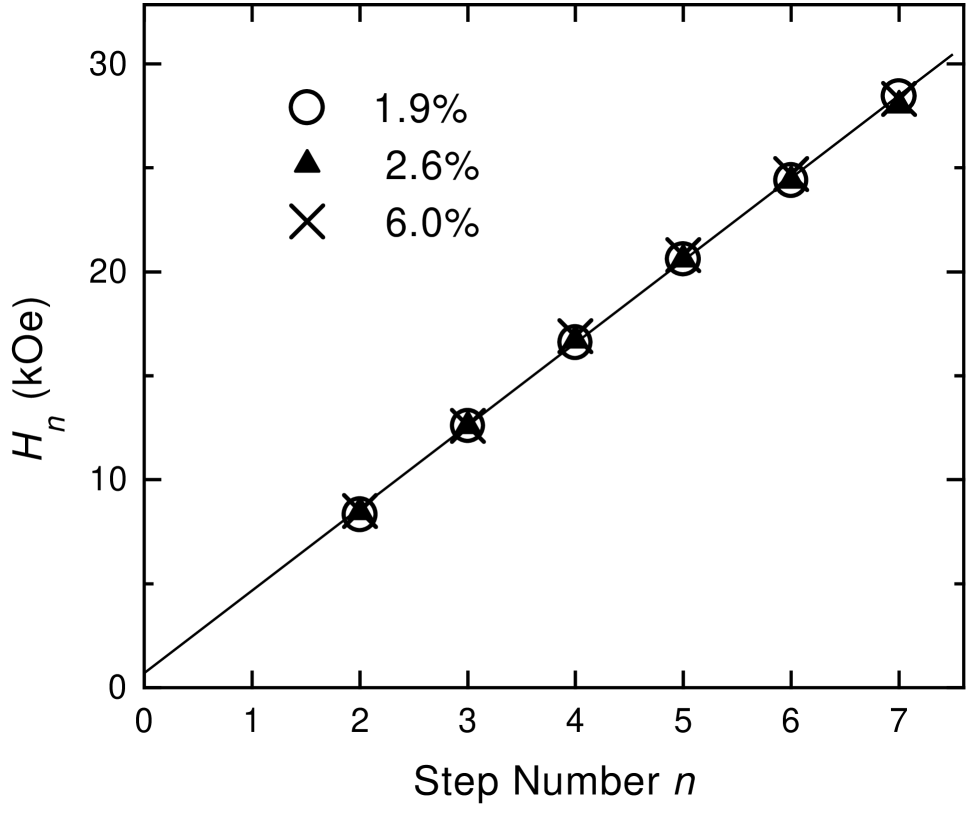
FIG. 4.: The fields $H_{n}$ at the MSTs from pairs as a function of the step number $n$. The straight line represents Eq. (1) with the average values for $J$ and $\Delta_{n}$.

In all three samples the pair and triplets involving the exchange constant $J$ gave rise to distinct ramps on which well-resolved MSTs were observed. No additional ramps or MSTs from any other exchange constant were found. The single-$J$ model therefore seems to be appropriate for describing the magnetization curves. Additional evidence that the corrections for the single-$J$ model are small will be discussed later.

The fields $H_{n}$ at the pair MSTs were obtained from the peaks in Fig. 2. Figure 4 shows a plot of these fields for the three samples. Because the first MST was not observed, the plot is only for $n=2$–7. It is evident that $H_{n}$ is approximately linear in $n$, so that Eq. (1) with a constant $\Delta_{n}$ is a good approximation (see Ref. [15]).

The values for $J$ obtained from least squares fits to Eq. (1), holding $\Delta_{n}$ constant, were the same for all three samples within 2%. The average value was $J/k_{B}=-0.264$ K. The values for $\Delta_{n}$ obtained from fits of the three data sets to Eq. (1) were all positive. The average was $\Delta_{n}=0.69$ kOe, which is only a fraction of the spacing $\Delta H=4$ kOe between successive MSTs.

As far as further neigbor exchange interactions are concerned, we can say the following. The data show that any other AF exchange constant is at least a factor of 3 smaller than the observed $J$. If this were not the case, another noticeable ramp ending between 10 kOe and 30 kOe should have been present, leading to a change of slope in this field region. Such a change of slope was not observed. Furthermore, the observed MSTs show only a small amount of non-thermal broadening and $\Delta_{n}$ depends only weakly on $x$. These observations show that the magnetization above about 10 kOe is very little affected by other (smaller) exchange constants originating from further neigbors.

The following arguments indicate that the quoted value $J/k_{B}=-0.264$ K corresponds to the largest AF exchange constant. The 0.6 K data in Fig. 3 show no other MSTs or ramps in fields up to 175 kOe. This means that if there were any larger AF exchange constant, its magnitude should have exceeded 12 K. On the other hand the Curie-Weiss temperatures discussed below rule out such a large AF exchange constant. Thus, the observed MSTs gave the largest $J$.

Our final result is then that the dominant exchange constant has the value $J/k_{B}=-0.264\pm 0.018$ K. The 7% uncertainty is motivated by the calculations of the corrections mentioned in Sec. II, and the observation that further neighbor interactions affect the MSTs very little. This $J$ for Pb_1-xEu_xTe is only slightly larger than $-0.24$ K for Pb_1-xEu_xSe.[8] There was no measurable dependence of $J$ on $x$ in the present Pb_1-xEu_xTe samples (see Fig. 4), despite the fact that the band gap changes by nearly a factor of 2 as $x$ changes from 1.9 to 6.0%.[1] The fields at the three observed MSTs from OTs, above 32 kOe, are close to those expected from the value of $J$ derived from the pair steps. This means that the exchange constants for pairs and triplets are the same (within a few percents), as expected.

Low-field susceptibility data were taken at temperatures down to 2 K. The most accurate result for $\theta$ was for the sample with $x=6.0$%. With the usual assumptions [16] the value $\theta=-1.9$ K gave $J/k_{B}=-0.25$ K (assuming $J=J_{1}$). The results for the other two samples, with lower $x$, were $J/k_{B}=-0.30$ ($x=2.6\%$) and $-0.22$ K ($x=1.9\%$), but these were judged to be less accurate. The values found by Gorska et al. [3] were $J/k_{B}=-0.38$ K for $x=3\%$, and $-0.27$ K for $x=6\%$. The spread in the values of $J$ obtained from $\theta$ shows that that the experimental uncertainty is not negligible, especially for low concentrations. Determining $J$ from the Curie-Weiss $\theta$ has several other drawbacks. First, it assumes that the distribution of the Eu ions is random, which, as discussed later, may not be exactly true for Pb_1-xEu_xTe. Second, $\theta$ depends on all exchange constants. Third, even when one $J$ is much larger than all the others, its estimate depends on whether it is identified as $J_{1}$ (between NNs, as was done above) or $J_{2}$ (between NNNs). The identification of $J$ as $J_{2}$ would lead to an estimate of $J$ which is larger by a factor of 2 compared to $J=J_{1}$. The MSTs method is a direct determination of $J$, which is independent of the identification of $J$, and is also independent of the spatial distribution of the Eu ions.

Gorska et al. [3] also determined $J$ by analyzing the magnetization curve at 4.2 K. At this relatively high temperature, $k_{B}T=16|J|$, the MSTs are not resolved, and the ramps due to pairs and OTs do not stand out clearly. The analysis which was performed fitted the magnetization curve to a sum of two contributions: one from singles and the other from “PAIRS”. The value for $J$ was deduced from the PAIR contribution. The results were $J/k_{B}=-0.43$ K for $x=3\%$, and $-0.50$ K for $x=6\%$. The reason that these values are much higher than our value of $-0.264$ K, is that the assumed “PAIRS” actually included not only true pairs but also triplets, quartets, and larger clusters. Since the saturation field of a cluster increases with cluster size, the net effect was that the assumed PAIRS saturated at higher fields than true pairs. This caused the deduced $J$ to be higher than the true $J$. It is probably significant that the fitted $J$ was larger for $x=6\%$ than for $x=3\%$, because the percentage of large clusters increases with $x$.

C Eu distribution and the identity of $J$

FIG. 5.: Comparison between the measured magnetization curve at 20 mK with computer simulations based on the $J_{1}$ - and $J_{2}$ models. a) $x$ = 1.9%. b) $x$ = 2.6%.

FIG. 6.: Comparison between the measured magnetization curve for $x$ = 6.0% and computer simulations based on the $J_{1}$ - and $J_{2}$ models. a) $T=20$ mK, b) $T=0.6$ K.

The identity of the dominant AF exchange constant $J$, whether it is $J_{1}$ for NNs or $J_{2}$ for NNNs, is a significant issue. Normally, exchange constants decrease rapidly with distance, so that the dominant $J$ is between NNs. This expected normal behavior has been found in all Mn-based II–VI DMS.[6] On the other hand, in pure EuTe the largest exchange constant is $J_{2}$, which is antiferromagnetic with a value of about $-0.2$ K. The exchange constant $J_{1}$ in EuTe is ferromagnetic and smaller in magnitude.[17, 18] Thus, after $J$ was measured in the present work, it was still not obvious whether it was $J_{1}$ or $J_{2}$.

To address this problem the measured magnetization curves were compared with computer simulations based on the two competing hypotheses: $J=J_{1}$ ($J_{1}$ model), or $J=J_{2}$ ($J_{2}$ model). Both models are single-$J$ models. The simulations were similar to those in Ref. [8] except that they also included the quartets and the others. We also chose to normalize the magnetization curves to the saturation value $M_{0}$ rather than to the data point at the highest field (see Ref.[19]). The key assumption in the simulations was that the Eu ions were distributed randomly, i.e., the probability of occupation of each cation site in the crystal was $x$. The simulations with the $J_{1}$ - and $J_{2}$ models lead to different magnetization curves, essentially because there are 12 NNs but only 6 NNNs in the fcc cation lattice. This difference means that in the $J_{2}$ model the number of singles is higher and the populations of pairs and larger clusters are lower.

Figure 5 compares the magnetization curves at 20 mK, for $x=1.9$ and 2.6%, with simulations based on the two models. To account for the somewhat larger observed width of the MSTs than that expected from thermal broadening alone, the simulations of data at 20 mK used an effective temperature of 100 mK. This change has no effect on the discussion below. [8] The simulation of data at 0.6 K were made with the actual temperature. From the figure it is clear that the $J_{1}$ model simulation is closer to the data, but even this model fails to reproduce the measured curves exactly. The deviations are more pronounced for $x=2.6$%. The observed initial rise of $M$ is smaller than predicted, indicating that even the $J_{1}$ model overestimates the number of singles. Furthermore, the observed slope between 30 and 40 kOe is higher than predicted by both models. This means that there are more triplets and/or larger clusters than calculated using a random distribution. The same features are also seen in Fig. 6, which is for $x=6.0\%$ at 20 mK and at 0.6 K. The $J_{1}$ model is closer to the data, but even compared to this model the actual number of singles is lower and the number of triplets and/or larger clusters is higher.

These results indicate that the local Eu concentration in the vicinity of a typical Eu ion is higher than the average concentration for the sample as a whole. Thus, the Eu ions tend to bunch together, leading to an inhomogeneous Eu distribution. The size of the regions with higher Eu concentration cannot be inferred from analysis of the magnetization curves alone. The microprobe measurements (Sec. III) examined the concentration variations on length scales greater than a few $\mu$m. The attempt to account for the magnetization curves by using the microprobe results as the local concentration profile was unsuccessful. This is particularly evident for the sample with $x=6.0\%$, in which the microprobe concentration showed very little variation with position. Combining the analysis of the magnetization data with the microprobe results we conclude that the length scale of the concentration inhomogeneities was smaller than a few $\mu$m.

A quantitative measure of the degree to which the Eu ions bunch together can be obtained by introducing the concept of a local concentration $x_{L}$. The simple picture which is behind this concept presumes that there is a typical local concentration in the vicinity of a typical Eu ion. It can differ from the average concentration $x$ for the sample as a whole. The populations of the various clusters are calculated assuming that the probability of occupation of each cation sites in the vicinity of a Eu ion is $x_{L}$ instead of $x$. The value of $x_{L}$ is found by varying the Eu concentration in the simulation until a match with the experimental magnetization curve is achieved. Using this procedure the following results were obtained for the samples with $x$ = 1.9, 2.6 and 6.0%. With the $J_{1}$ model, $x_{L}$ = 2.5, 3.8, and 7.7%, respectively. With the $J_{2}$ model, $x_{L}$ = 4.7, 7, and 14%, respectively. Obviously, a much smaller difference between $x_{L}$ and $x$ is required to achieve agreement with the $J_{1}$ model.

In the discussion above, we have assumed that the deviations of the data from a single-$J$ model were due to the assumption of a random distribution. An alternative would be to question the validity of the single-$J$ model itself. It is known that long range exchange interactions between further neighbors can influence the magnetization process in diluted magnetic semiconductors.[10, 20, 21, 22] Such long-range interactions may be important in small-gap DMS, such as the present system. The key question here is whether long-range interactions could have affected the magnetization in fields above 10 kOe significantly, since the conclusion of a non-random distribution was based on the data at these high fields, especially above 30 kOe.

The effects of further neighbors (distant neighbors) on the magnetization curve have been treated using several approximate methods. One approach starts from the clusters in the single-J model, but then subjects these clusters to effective fields arising from further neighbors.[10] Alternative approaches use more general spin clusters which include further neighbors within the clusters, so that the intracluster interactions already include the further neighbors.[20, 21, 22] Since our analysis started from the single-J model, the first approach (effective fields acting on the single-J clusters) is more convenient here. The effective fields from further neighbors slow down the alignment of spins which are singles, and they shift and broaden the ramps and MSTs arising from larger clusters (e.g. pairs and triplets). These effects increase with the Eu concentration $x$. We now present several arguments which indicate that in the present work the further-neighbor effective fields were far too weak to significantly affect the magnetization curve well above 10 kOe.

At 20 mK the magnetization rises very quicly at low $H$ (Figs. 1 and 5). The singles seem to become practically saturated at about 2 kOe. Considering that the cubic crystal field anisotropy also slows down the alignment of the singles,[8] we conclude that typical further-neighbor effective fields acting on singles are less than about 1 kOe. Such weak effective fields are unlikely to have a significant effect on the magnetization well above 10 kOe.

The fields $H_{n}$ at the MSTs from pairs are shifted by the further-neighbors effective fields.[10] These shifts, included in the $\Delta_{n}$ of Eq. (1), are predicted to increase with $x$. However, the results in Fig. 4 indicate that the $\Delta_{n}$ are all less than about 1 kOe. Also, despite the factor-of-three change in $x$, the fields $H_{n}$ do not vary by more than a fraction of 1 kOe. This means that typical further-neighbor effective fields acting on pairs were no more than a fraction of a kOe, even for the sample with $x=6$%. Typical effective fields acting on triplets and quartets should not be higher by more than a factor of 2 or so. It is very unlikely that such weak effective fields will have a significant effect on the magnetization curve well above 10 kOe.

The spread in the magnitude of the effective field acting on different pairs gives rise to a broadening of the MSTs from pairs.[10] Such a broadening should increase with $x$. The fact that well resolved MSTs were observed even for $x=6$% means that the spread in the effective fields was considerably smaller than the 4 kOe separation between the MSTs. Thus not only was the average effective field small, but the spread was also small. Such a distribution of effective fields should not have a significant effect on the magnetization curve well above 10 kOe.

The final argument in support of a non-random distribution is based on an analysis of the change in the slope of the magnetization curve near 43 kOe. This change occurs when the triplet ramp ends. (The change in slope is visible in Figs. 1 and 5, but is clearer in expanded plots of the magnetization curves at 20 mK.) The magnitude of this change in slope is related to the number of triplets. Analysis of the data in all three samples indicates a significantly larger number of triplets than predicted assuming a random distribution. Further-neighbor interactions cannot account for the significanly larger change in slope which was observed.

Claims of a non-random distribution in II-VI DMS have been made more than a decade ago (see e.g. Ref. [23]). However, MST studies showed that the distribution in such DMS was in fact random.[24, 6] Here, in our Pb_1-xEu_xTe samples, we find a small non-randomicity which we believe to be genuine. In Ref. [8] (Pb_1-xEu_xSe) deviations of the data with the $J_{1}$-model were also found, but the simulations included only clusters up to triplets. A re-analysis of those data with our improved model, which includes quartets and an approximation for larger clusters, still does not lead to perfect agreement. As in the present work, good agreement with the data is obtained if small deviations from a random distribution are assumed (and that $J=J_{1}$). The non-randomicity in the Pb_1-xEu_xSe samples is smaller than that in the Pb_1-xEu_xTe samples.

Returning to the issue of the identity of $J$ , there are two possibilities. Either $J$ is $J_{1}$ in which case the Eu ions have only a fairly modest tendency to bunch together, or $J$ is $J_{2}$ with a very large increase of the local Eu concentration. Because the usual distribution of magnetic ions in a DMS is random,[6] we believe that the first possibility is more likely. On this basis we tentatively identify $J=-0.264\pm 0.018$ K as $J_{1}$. However, since the actual distribution is unknown, the possibility that it is $J_{2}$ cannot be excluded entirely. If one accepts that $J$ is $J_{1}$ then the exchange constants in Pb_1-xEu_xTe when $x$ is low are very different from those in EuTe.[17, 18] Such a difference may be the result of a different band structure and a different position of the Eu levels.

V Acknowledgments

We are grateful to C. Merlet of the University of Montpellier II for assistance in the microprobe measurements, and to M.T. Liu for help in some of the magnetization measurements. The work in Brazil was supported by CNPq, FAPESP, and FINEP. The work in the U.S. was partially supported by NSF Grants Nos. DMR-9219727 and INT-9216424. The work in France was supported by CNRS. The work in Poland was supported by the Polish Committee for Scientific Research. The Francis Bitter National Magnet Laboratory was supported by NSF.

REFERENCES

- [1] G. Bauer and H. Pascher in Diluted Magnetic Semiconductors, edited by Mukesh Jain, World Scientific, Singapore (1991).
- [2] G.B. Bacskay, P.J. Fensham, I.M. Ritchie, and R.N. Ruff J. Chem. Phys. Solids 30, 713 (1969).
- [3] M. Gorska, J.R. Anderson, G. Kido and Z. Golacki, Solid State Commun. 75, 363 (1990).
- [4] M. Gorska, J.R. Anderson, G. Kido, S.M. Green and Z. Golacki, Phys. Rev. B 45, 11702 (1992).
- [5] J.R. Anderson, G. Kido, Y. Nishina, M. Gorska, L. Kowalczyk and Z. Golacki, Phys. Rev. B 41, 1014 (1990).
- [6] Y. Shapira, J. Appl. Phys. 67, 5090 (1990); Y. Shapira in Semimagnetic Semiconductors and Diluted Magnetic Semiconductors, edited by M. Averous and M. Balkanski (Plenum, New York, 1991).
- [7] For a recent review of the magnetization-steps method see V. Bindilatti, N.F. Oliveira, Jr., E. ter Haar, and Y. Shapira, in the Proc. of the 21st Intl. Conf. on Low Temp. Physics (LT21), Prague, 1996: Czech. J. Phys. 46 Suppl. 6, 3255 (1996).
- [8] V. Bindilatti, N.F. Oliveira Jr., Y. Shapira, G.H. McCabe, M.T. Liu, S. Isber, S. Charar, M. Averous, E.J. McNiff, Jr., Z. Golacki, Phys. Rev. B 53, 5472 (1996).
- [9] M.T. Liu, Y. Shapira, E. ter Haar, V. Bindilatti and E.J. McNiff, Jr., Phys. Rev. B 54, 6457 (1996). More recently these results were extended to quartets composed of spins S= 7/2 (E. ter Haar and M.T. Liu, unpublished).
- [10] B.E. Larson, K.C. Haas, and R.L. Aggarwal, Phys. Rev. B 33, 1789 (1986).
- [11] R.E. Behringer, J. Chem. Phys. 29, 537 (1958); M.M. Kreitman and D.L. Barnett, ibid 43, 364 (1965).
- [12] V, Bindilatti and N.F. Oliveira, Jr., Physica, B 195-196, 63 (1994).
- [13] E. ter Haar, R. Wagner, C.M.C.M. van Woerkens, S.C. Steel, G. Frossati, L. Skrbek, M.W. Meisel, V. Bindilatti, A.R. Rodrigues, R.V. Martin and N. F. Oliveira Jr., J. Low Temp. Phys. 99, 151 (1995).
- [14] Quantum Design Inc, San Diego, CA - USA.
- [15] Detailed examination of the observed spacings between successive MSTs shows that, for each of the samples, these spacings vary relative to the mean value by up to 10%. Some of this variation is due to experimental uncertainties but the main cause is probably the cubic crystal field anisotropy. In that case, in Eq. (1) is not exactly independent of . Nevertheless, making a fit with constant should give quite an accurate value for .
- [16] J. Spalek, A. Lewicki, Z. Tarnawski, J.K. Furdyna, R.R. Galazka, and Z. Obuszko, Phys. Rev. B 33, 3407 (1986).
- [17] N.F. Oliveira, Jr., S. Foner, Y. Shapira, and T.B. Reed, Phys. Rev. B 5, 2634 (1972).
- [18] A. Mauger and C. Godart, Phys. Rep. 141, 51 (1986).
- [19] The only significant difference between the two normalization procedures was for at 20 mK, because was not saturated at the maximum field of 50 kOe. The normalization in this case was based on the good match between the data at 20 mK and 0.6 K for fields above 15 kOe, as shown in Fig. 3(b). It was assumed that this good match persisted above 50 kOe.
- [20] C.J.M. Denissen and W.J.M. de Jonge, Solid State Commun., 57, 503 (1986).
- [21] A. Twardowski, H.J.M. Swagten, W.J.M. de Jonge and M. Demianiuk, Phys. Rev. B 36, 7013 (1987).
- [22] T.Q. Vu, V. Bindilatti, Y. Shapira, E.J. McNiff, C.C. Agosta, J. Papp, R. Kershaw, K. Dwight and A. Wold, Phys. Rev B 46, 11617 (1992).
- [23] R.R. Galazka, S. Nagata and P.H. Keesom, Phys. Rev. B 22, 3344 (1980).
- [24] Y. Shapira, S. Foner, D.H. Ridgley, K. Dwight and A. Wold, Phys. Rev. B 30, 4021 (1984).