Cooling dynamics of a dilute gas of inelastic rods: a many particle simulation

Abstract

We present results of simulations for a dilute gas of inelastically colliding particles. Collisions are modelled as a stochastic process, which on average decreases the translational energy (cooling), but allows for fluctuations in the transfer of energy to internal vibrations. We show that these fluctuations are strong enough to suppress inelastic collapse. This allows us to study large systems for long times in the truely inelastic regime. During the cooling stage we observe complex cluster dynamics, as large clusters of particles form, collide and merge or dissolve. Typical clusters are found to survive long enough to establish local equilibrium within a cluster, but not among different clusters. We extend the model to include net dissipation of energy by damping of the internal vibrations. Inelatic collapse is avoided also in this case but in contrast to the conservative system the translational energy decays according to the mean field scaling law, $E(t)\propto t^{-2}$, for asymptotically long times.

]

I Introduction

In a recent paper [1], hereafter referred to as I, we discussed the properties of inelastic two particle collisions, starting from a Hamiltonian model for one dimensional elastic rods. Within this model, the coefficient of restitution $\epsilon$ does not only depend on the relative velocity of the colliding particles, but in addition becomes a stochastic quantity, depending on the state of excitation of the internal vibrations. Here we extend the analysis to a discussion of the many body dynamics of a one-dimensional gas of granular particles, modelled as elastic rods. We concentrate on dilute granular systems in the ”grain inertia” regime, where two particle collisions dominate the dynamics. It was shown in I that successive collisions are to a very good approximation uncorrelated, so that the many body dynamics is a random Markov process. Consequently, the collisions are simulated by a Monte Carlo algorithm: velocities are updated with a random coefficient of restitution, drawn from the appropriate probability distribution. In between collision events, particles move freely like in an event driven algorithm.

We focus here on the cooling properties of a large system (10000 particles) in the inelastic regime and refer to cooling as the decay of translational energy with time. We observe the evolution of spatial structures, without running into problems with inelastic collapse, which is always avoided by the algorithm. The most prominent spatial structures are large clusters of particles, which are seen to form and decay by colliding with other clusters. The velocity distribution within a cluster is to a good approximation Maxwellian, whereas the global velocity distribution shows significant deviations from Maxwellian, indicating that local equilibrium has been established within a cluster, but not among different clusters.

The model is extended to include net dissipation, i.e. irreversible energy loss, in a phenomenological way by simply introducing a single relaxation time for the decay of the energy of internal vibrations. The final state of this model is one big cluster with all particles at rest. The dynamics with dissipation resembles a deterministic system (i. e. with constant coefficient of restitution) as long as no inelastic collapse is threatening. When the collision frequency increases dramatically, then ultimately the time between collisions will become smaller than the decay time for the internal energy, so that the vibrations no longer decay in between collisions. Then the model effectively reduces to the above stochastic one without dissipation and no inelastic collapse occurs. The kinetic energy of translation follows on average the mean field scaling law $E(t)\propto t^{-2}$.

Several groups have simulated onedimensional granular media using event driven algorithms with constant coefficient of restitution. For $(1-\epsilon)\geq const./N$ a divergence of the collision frequency in finite time, i.e. inelastic collapse is observed. This leads to a breakdown of the algorithm and one either has to restrict oneself to the quasielastic regime, where $\epsilon$ is sufficiently close to one or additional assumptions about the dynamics of clusters have to be made. Bernu and Mazighi [3] investigate a column of beads colliding with a wall. McNamara and Young [4] and Sela and Goldhirsch [5] discuss the cooling dynamics of a granular gas in the quasielastic regime. They observe the evolution of spatial structures and a bimodal velocity distribution. The critical wavelength of the instability is related to the minimum number of particles for inelstic collapse to occur, given a fixed value of $\epsilon$. Clement et al. [6] and Luding et al. [7] study a vertical column of beads in a gravitational field with a vibrating bottom plate. For $\epsilon$ close to one they observe a fluidization transition, whereas for $\epsilon\ll 1$ a bifurcation scenario is seen to take place. The latter has also been observed by Luck et al. [8] for a single bead on a vibrating plane.

All of the above simulations use a coefficient of restitution which is independent of the impact velocity whereas experiments on ice spheres reveal a velocity dependence of $\epsilon$ [9]. There have also been several attempts to calculate the velocity dependence of the coefficient of restitution by extending the static theory of Hertz [10] to viscoelastic behaviour. One either assumes a phenomenological damping term [11] in the equation of motion for the deformation or alternatively uses a quasistatic approximation [12, 13] for low relative impact velocities. As a result of either approximation the coefficient of restitution becomes velocity dependent. Simulations of large systems with strongly inelastic collisions have been performed with this model [14].

Another approach is based on phenomenological wave theory. Here one assumes that two colliding bodies do not vibrate before collision and that the impact triggers a travelling elastic wave in both of them. For one dimensional rods this ansatz yields [15] $\epsilon=l_{1}/l_{2}$, independent of the relative velocity of the colliding particles. Here $l_{1}$ ($l_{2}$) denotes the length of the shorter (longer) rod. As shown in I, these results are contained in our model.

Our paper is organized as follows. In the next section we review the model of I, discuss the probability distribution of $\epsilon$ and define the algorithm for the many body dynamics. Results of simulations are presented in sec. III. We first discuss global quantities, like the time decay of the kinetic energy and the total number of collisions as a function of time. Subsequently we analyse the local structure with help of the paircorrelation function and discuss the formation and decay of particle clusters, as well as the distribution of the particles’ velocities. In sec. IV the model with dissipation of vibrational energy is introduced. Finally in sec. V we summarize our results and give an outlook to forthcoming work.

II Markovian dynamics of inelastic rods

We first review the Hamiltonian model of I and summarize the properties of two particle collisions. We then show that the transition probabilities of the resulting Markov process obey detailed balance and introduce the algorithm for the dynamics of the many-body system.

A Two-particle collisions

Our starting point are the Hamiltonian equations of motion of a system of $N$ elastic rods of homogeneous mass density. The particles are placed on a ring of circumference $L$. Each rod is characterized by its length $l_{i}$, total mass $m_{i}$ and centre of mass position $R_{i}(t)$. Its vibrational excitations are described by $N_{mod}$ normal modes $q_{i}^{\nu}(\nu=1,\ldots,N_{mod})$ of wavenumber $k_{i,\nu}=\pi\nu/l_{i}$ and frequency $\omega_{i,\nu}=ck_{i,\nu}$. The only important material parameter for our model is the sound velocity $c$. We model collisions of the rods by a short range repulsive potential $V(r)=B\exp{(-\alpha r)}$, which depends on the momentary end-to-end distance $r$ between the colliding rods, thus coupling translational and vibrational degrees of freedom. We shall be interested in the hard core limit, which can be achieved by letting $\alpha\to\infty$ . The total Hamiltonian of our model reads:

$${\cal H} = {\cal H}_{bath}\left\{p_{i}^{(\nu)},q_{i}^{(\nu)}\right\}+{\cal H}_{tr}\left\{P_{i}\right\}+{\cal H}_{int}\left\{R_{i},q_{i}^{(\nu)}\right\}$$ (1)

$$= \sum\limits_{i=1}^{N}\sum\limits_{\nu=1}^{N_{mod}}\left\{\frac{{p_{i}^{(\nu)}}^{2}}{2m_{i}}+m_{i}\omega_{i,\nu}^{2}\frac{{q_{i}^{(\nu)}}^{2}}{2}\right\}+\sum\limits_{i=1}^{N}\frac{P_{i}^{2}}{2m_{i}}+$$ (3)

$$\sum\limits_{i=1}^{N-1}Be^{-\alpha\left(R_{i+1,i}+\sqrt{2}\sum\limits_{\nu}\left(q_{i+1}^{(\nu)}-(-1)^{\nu}q_{i}^{(\nu)}\right)\right)}\quad.$$

Here $R_{i+1,i}=R_{i+1}-R_{i}-(l_{i+1}-l_{i})/2$ is the end-to-end distance of two undeformed neighbouring rods and $P_{i}(t)$ and $p_{i}(t)$ denote the conjugate momenta for the centre of mass and the amplitude of vibration. The first term, ${\cal H}_{bath}$, models the internal vibrations, the second term, ${\cal H}_{tr}$, the translational motion, and the third term, ${\cal H}_{int}$, the interaction between the rods.

In I we have analysed the statistical properties of two-particle collisions by numerically integrating the full Hamiltonian dynamics for the case $N=2$ with length ratio $\gamma=l_{1}/l_{2}$. The main results are the following. Equipartition among the vibrational states of a rod is achieved fast (after about five collisions) as compared to the relaxation of the translational velocity, which happens on a time scale of about 80 collisions. The coefficient of restitution of two successive collisions is to a very good approximation uncorrelated. Based on these observations a simplified description was achieved in I by integrating out the internal degrees of freedom, which can be done exactly for a single two particle collision. One is left with an effective equation of motion for the rescaled relative velocity of the two rods $w(\tau)=\dot{R}_{2,1}(t)/\dot{R}_{2,1}(0)-1$. Here $\tau=ct/l$ and $l=2l_{1}l_{2}/(l_{1}+l_{2})$ denotes an effective length which is always chosen much larger than the range of the potential, i.e. $\alpha l\gg 1$. Based on the observation of fast equipartition among the vibrational states, these are modelled by a thermalized bath, characterized by a temperature $T_{B}=E_{bath}/N_{mod}$, where the vibrational energy of a rod is given by the sum of the energies of the individual modes: $E_{bath}=\sum_{\nu=1}^{N_{mod}}E_{\nu}$. Thus $q_{i}^{\nu}(0)$ and $p_{i}^{\nu}(0)$ are taken as independent, canonically distributed random variables

$$\langle q_{i}^{(\nu)}(0)\rangle = \langle p_{i}^{(\nu)}(0)\rangle\,\,=\,0$$ (4)

$$\left\langle(q_{i}^{(\nu)}(0))^{2}\right\rangle = \left\langle\left(\frac{p_{i}^{(\nu)}(0)}{m_{i}\omega_{i,\nu}}\right)^{2}\right\rangle=\frac{T_{B}}{m_{i}\omega_{i,\nu}^{2}}.$$ (5)

Under these assumptions the relative velocity $w(\tau)$ obeys a stochastic equation of motion

$$\frac{d}{d\tau}w(\tau) = \frac{1}{\kappa}\exp\bigg{\{}\kappa\big{(}\tau-\tau_{0}-w(\tau)-$$ (7)

$$\quad\sum\limits_{i=1}^{2}\sum\limits_{n=1}^{\infty}w(\tau-n\Gamma_{i})+q(\tau)\big{)}\bigg{\}},$$

where $\kappa=-\frac{\alpha l}{c}\dot{R}_{2,1}(0)$ and $\tau_{0}=\alpha R_{2,1}(0)/\kappa$. The coefficient of restitution is given by

$$\epsilon=\lim_{\tau\to\infty}w(\tau)-1$$ (8)

and thus becomes a stochastic variable, depending on the state of the vibrational bath before the collision. $q(\tau)$ is a Gaussian random noise with zero mean and covariance

$$C_{q}(\tau) = \langle q(\tau^{\prime})q(\tau^{\prime}+\tau)\rangle$$ (9)

$$= \Biggl{\{}\sum_{i=1}^{2}\frac{1}{2\Gamma_{i}}\Biggl{(}\tau-\frac{\Gamma_{i}}{2}-\Gamma_{i}\sum_{n=1}^{\infty}\theta(\tau-n\Gamma_{i})\Biggr{)}^{2}-$$ (11)

$$\quad\frac{\Gamma_{1}\Gamma_{2}}{24}\Biggr{\}}\sigma^{2},$$

$$\sigma^{2} = \frac{T_{B}}{2E_{tr}}.$$ (12)

Here, $\theta$ denotes the Heaviside step function and $E_{tr}=\mu(\dot{R}_{2,1}(0))^{2}/2$ is the translational energy of the colliding rods in their center of mass frame of reference. The $\Gamma_{i}$ which appear in eqs. (7) and (9) are determined by the length ratio $\gamma$ of the rods according to $\Gamma_{1}=1+\gamma$ and $\Gamma_{2}=1+\frac{1}{\gamma}$ and $\mu=m_{1}m_{2}/(m_{1}+m_{2})$ is the effective mass. The stochastic process $\{q(\tau)\}$ is simply related to two periodic brownian bridge processes [16] with periods $\Gamma_{1}$ and $\Gamma_{2}$ respectively.

In the hard core limit ($\kappa\to\infty$) the stochastic equation for the rescaled relative velocity $w(\tau)$ (eq. (7)) can be solved by saddle point methods, yielding

$$w(\tau) = \max\left(0,f(\tau)\right),\quad\mbox{where}$$ (13)

$$f(\tau) = \max_{0\leq\tau^{\prime}\leq\tau}\biggl{\{}\tau^{\prime}-\tau_{0}-\sum_{i,\nu}w(\tau^{\prime}-\nu\Gamma_{i})+q(\tau^{\prime})\biggr{\}}.$$ (14)

The duration of the collision as well as the final velocity are stochastic variables. The collision is ended when the memory terms in eq. (13) overcompensate the gain from the other terms $\tau^{\prime}-\tau_{0}+q(\tau^{\prime})$, which are on average increasing.

B Transition Probability

The results of the preceding section are interpreted as a Markov process in discrete time, which accounts for transitions of the translational energy upon successive collisions. During a collision $E_{tr}$ changes to a new value $E^{\prime}_{tr}=E_{tr}\epsilon^{2}$. The probability for this transition is determined by the probability density for the coefficient of restitution $p_{\beta}(\epsilon)$ according to

$$p_{\scriptscriptstyle T_{B}}(E_{tr}\rightarrow E^{\prime}_{tr}) = \frac{1}{2\epsilon E_{tr}}p_{\beta}\!(\epsilon)\Biggr{|}_{\epsilon=\sqrt{\frac{E^{\prime}_{tr}}{E_{tr}}}}\quad,$$ (15)

$$\beta = \frac{E_{tr}}{T_{B}}$$ (16)

($T_{B}$ here denotes the bath temperature of both rods, under the assumption that the temperatures are equal. If that is not the case, one would have to replace the index $\beta$ by two indices $\beta_{1}$ and $\beta_{2}$. Here, we use only one index for notational simplicity.)

Changes in the bath temperature are not independent, but determined by energy conservation:

$$T^{\prime}_{B}=T_{B}+\frac{1-\epsilon^{2}}{2N_{mod}}E_{tr}$$ (17)

The stationary state of the Markov process is known: after cooling, the system of two particles, each equipped with an internal bath, evolves into a stationary state with a Boltzmann distribution for $E_{tr}$

$$p_{\scriptscriptstyle T_{B}^{0}}^{stat}(E_{tr})=\frac{1}{T_{B}^{0}}\exp\left(-\frac{E_{tr}}{T_{B}^{0}}\right)$$ (18)

with the bath temperature $T_{B}^{0}=\frac{E_{tot}}{2N_{mod}+1}$ where $E_{tot}$ is the total energy of the system.

It can be proven [17] that this collision process obeys detailed balance, which gives the following relation for $p_{\beta}(\epsilon)$ (this relation only holds if the temperature of both rods is indeed equal, i. e. $\beta_{1}=\beta_{2}=\beta$):

$$p_{\beta}(\epsilon)e^{-\beta}=p_{\epsilon^{2}\beta}\left(\frac{1}{\epsilon}\right)e^{-\epsilon^{2}\beta}$$ (19)

When the temperatures of the baths of oscillators are zero, i. e. $q(\tau)=0$ for all $\tau$, the collision is deterministic. For this case, the coefficient of restitution is equal to $\gamma$, the ratio of the lengths of the rods (see I and [15]). Thus in the limit of small temperatures, $p_{\beta}(\epsilon)$ should approach a $\delta$-Function centered around $\gamma$.

At large temperatures, on the other hand, simulations suggest the (quite sensible) result that $p_{\beta}(\epsilon)$ is a uniform distribution, i. e. all possible $\epsilon$’s are equally probable.

It can be shown from equation (13) that for $\gamma=1$ the collision is always deterministic, i. e. $\epsilon=1$ for any realisation of the stochastic process ${q(\tau)}$. This interesting result will have implications on our setup of the simulations (see sec. II C).

C Algorithm

We now consider the dynamic evolution of $N$ particles on a ring of circumference $L+\sum_{i=1}^{N}l_{i}$. $L$ is thus the total length of the interparticle spacings. For the following arguments the actual lengths of the particles are unimportant because the point in time when a collision occurs depends only on the end-to-end distance and the outcome of a collision depends only on the length ratio. In order to keep the notation simple we map the system to an equivalent one consisting of $N$ point particles on a ring of circumference $L$. Each particle is characterized by its position $R_{i}(t)$, its velocity $\dot{R}_{i}(t)$, the temperature of its internal bath $T_{B}^{(i)}(t)$. The $N_{mod}$ internal modes of one rod are represented by one degree of freedom only, namely $T_{B}^{(i)}=\sum_{\nu=1}^{N_{mod}}E_{i}^{\nu}/N_{mod}$. The rods are assigned alternating lengths such that the ratio $\gamma$ for each collision has a fixed value, in our case $0.8$. The ratio of masses is also given by $\gamma$, assuming the same homogeneous mass density for both kinds of rods. We choose rods of alternating length because due to the result given at the end of sec. II B a length ratio of $\gamma=1$ implies $\epsilon=1$ always which would correspond simply to a standard one dimensional hard sphere gas.

The model we use is a hybrid of an event driven algorithm and a Monte Carlo simulation. The particles move freely in between collisions, as in event driven algorithms. When two particles collide their states are updated stochastically, according to the distribution of $\epsilon$.

It is convenient to introduce dimensionless variables $x_{i}=R_{i}N/L$ and $v_{i}=\dot{R}_{i}\sqrt{\mu/T_{0}}$. $T_{0}$ serves as an energy scale and will be identified with the homogeneous initial granular temperature of the many particle system. Time is measured in units of $L\sqrt{\mu/T_{0}}/N$.

For the algorithm we only need relative distances and velocities

$$\Delta x_{i} = \biggl{\{}\begin{array}[]{rcl}x_{i+1}-x_{i}&\mbox{for}&1\leq i\leq N-1\\ N+x_{1}-x_{N}&\mbox{for}&i=N\end{array}$$ (22)

$$\Delta v_{i} = \biggl{\{}\begin{array}[]{rcl}v_{i+1}-v_{i}&\mbox{for}&1\leq i\leq N-1\\ v_{1}-v_{N}&\mbox{for}&i=N\end{array}$$ (25)

The algorithm is defined by iteration of the following steps:

1. Calculate the time difference $\Delta t$ for the next collision to take place:

   $$\Delta t=\min_{\{i|\Delta v_{i}<0\}}\left(-\frac{\Delta x_{i}}{\Delta v_{i}}\right)$$ (26)

   The pair of particles which is going to collide next is denoted by $(i_{0},i_{0}+1)$.

2. The relative distances of all particles are updated according to:

   $$\Delta x_{i}(t+\Delta t)=\Delta x_{i}(t)+\Delta v_{i}(t)\Delta t.$$ (27)

   For the designated pair $(i_{0},i_{0}+1)$ we obtain $\Delta x_{i_{0}}(t+\Delta t)=0$.

3. The kinetic energy of relative motion of the pair $(i_{0},i_{0}+1)$ as well as the mean local bath temperature are calculated according to $E_{tr}=\Delta v^{2}_{i_{0}}/2$ and $T_{B}=(T_{B}^{(i_{0})}+T_{B}^{(i_{0}+1)})/2$. Subsequently, a random value of $\epsilon$ is chosen from the probability distribution $p_{\beta}(\epsilon)$, presently calculated by numerically solving eq. (13) and applying eq. (8).

4. The bath temperatures and relative velocities are updated

   $$T_{B}^{(i_{0})}(t+\Delta t) = T_{B}^{(i_{0}+1)}(t+\Delta t)$$ (28)

   $$= T_{B}+\frac{1-\epsilon^{2}}{2N_{mod}}E_{tr}$$ (29)

   $$\Delta v_{i_{0}-1}(t+\Delta t) = \Delta v_{i_{0}-1}(t)+\frac{1+\epsilon}{2}\Delta v_{i_{0}}(t)$$ (30)

   $$\Delta v_{i_{0}}(t+\Delta t) = -\epsilon\Delta v_{i_{0}}(t)$$ (31)

   $$\Delta v_{i_{0}+1}(t+\Delta t) = \Delta v_{i_{0}+1}(t)+\frac{1+\epsilon}{2}\Delta v_{i_{0}}(t).$$ (32)

5. Continue with step 1.

III Simulations

Many-body simulations using the above algorithm have been performed to study the cooling dynamics of the system. More precisely, we focus here on the intermediate range of timescales where equipartition among the internal modes has already been achieved and the final equilibrium state of equipartition among all degrees of freedom is not yet reached. As shown below this time range extends over several orders of magnitude.

We assume that two particle collisions dominate the dynamic evolution of the system. This is justified for a dilute granular gas. The typical time of interaction in our model is given by $t_{int}=2l/c$, i.e. the time a signal needs to travel back and forth on a rod. Hence in principal, two colliding rods can interact with a third one. This will be highly unlikely, as long as the time between collisions is much longer than $t_{int}$. This requires $2l/c\ll L/(N|\dot{R}_{i+1,i}|)$. So either the length of the rods has to be chosen sufficiently small as compared to the mean distance $L/N$ or the initial velocities $|\dot{R}_{i+1,i}|$ should be small compared to the velocity of sound. The latter is a material parameter and can have quite high values for hard materials (e.g. for steel, $c\sim 10^{4}m/s$), favouring short interaction times. In a standard event-driven simulation inelastic collapse occurs when the number of particles is sufficiently large, resulting in a diverging collision frequency. This would clearly violate the condition that the time between two collisions is long compared to $t_{int}$. However, since our algorithm avoids the inelastic collapse, as will be discussed below, we will still make use of the assumption that three or more particle collisions will not be important.

A system of 10000 particles has been simulated and for most part a length ratio $\gamma=0.8$ has been used. We start from a spatially homogeneous distribution of particles having a maxwellian velocity distribution with $\langle\frac{\Gamma_{j}}{2}v_{j}^{2}\rangle=\frac{1}{2}$ ($j=1(2)$ stands for the shorter (longer) species of rods). We use $N_{mod}=1000$ vibrational modes per particle. Initially the internal bath temperature $T_{B}^{(i)}$ of each particle is set to 0.

Our simulations were performed on a cluster of Linux workstations with Pentium processors. The longest runs took about three weeks of computer time.

A Global quantities

Kinetic energy

The time development of the total kinetic energy, which is given by

$$E_{kin}=\sum_{i=1}^{N}\frac{\Gamma_{i}}{2}v_{i}^{2}$$ (33)

in our rescaled units, is shown in fig. 1, in comparison with results for the deterministic model with constant $\epsilon$.

FIG. 1.: Reduction of the kinetic energy per particle as a function of time. The curve for the deterministic coefficient of restitution breaks off because an inelastic collapse occured. The dot-dashed line shows the average energy per vibrational mode for the 50 particle run and illustrates that equipartition holds in the stationary state.

For small times the curves for the deterministic and the stochastic dynamics are rather similar. In the initial stage very little energy is stored in the internal modes and hence the coefficient of restitution is approximately given by the deterministic value. However the deterministic dynamics runs very quickly into the inelastic collapse, as can be seen from the total number of collisions which is shown as a function of time in fig. 2. When this happens, the simulation gets stuck so that the curve for the kinetic energy breaks off in fig. 1.

FIG. 2.: Number of collisions as a function of time. The inset shows a comparison of the deterministic model (dashed line) and the stochastic model (solid line). (The units on the axes of the inset are the same as on the regular axes.) The deterministic model quickly runs into the inelastic collapse, seen by the diverging number of collisions. The dotted lines shows the theoretical number of collisions as a function of time in the stationary state according to eq. (35) for the 10000 and the 50 particle runs. The data for the 50 particle run has been scaled by a factor of 100 in order to fit on the graph.

The stochastic dynamics shows completely different behaviour: The kinetic energy continues to decrease until equilibrium is reached, where $E_{kin}$ continues to fluctuate around the stationary value which is given by $E_{kin}^{stat}=E_{kin}(t=0)/(2N_{mod}+1)$. (The final state has not quite been reached for the 10000 particle run in the time interval that is shown in fig. 1.)

The final state of our stochastic model is a consequence of the idealised assumption that the total system be conservative. In a more realistic model of granular media one expects the particles to be at rest in the final state. In sec. IV we shall present a phenomenological extension of our model, which does take into account energy dissipation of the microscopic degrees of freedom. In the final state of the model with energy dissipation all particles are at rest.

Collision rate

Simple mean field arguments [5] have been used to derive scaling laws for the time evolution of kinetic energy and collision rate. One assumes that the particle velocities are uncorrelated and Gaussian distributed. For a constant coefficient of restitution one obtains $E_{kin}(t)\sim t^{-2}$ and $\dot{N}_{coll}\sim\ln t$. Neither scaling law fits our data, as can be seen from figs. 1 and 2. McNamara and Young [4] have already pointed out that the mean field scaling laws are only applicable in the quasi elastic regime, where no inelastic collapse occurs. Otherwise the assumption of uncorrelated Gaussian velocities breaks down. In the stochastic model we have additional fluctuations of the coefficient of restitution, which invalidate the derivation of the above scaling laws. Hence it is no surprise that the data disagree with these relations.

The rate of collisions becomes constant as the stationary state is approached, as can be seen from fig. 2. The average collision rate is given by $\dot{N}_{coll}=N\overline{\Delta v}/(2\overline{\Delta x})$. In the stationary state the velocities are indeed uncorrelated Gaussian variables, distributed according to

$$p_{j}(v)=\left(\frac{2\pi}{2N_{mod}+1}\right)^{-1/2}\exp{\left(-\frac{\Gamma_{j}v^{2}}{2(2N_{mod}+1)^{-1}}\right)},$$ (34)

where $j=1(2)$ again stands for the shorter (longer) type of rods. We assume $\overline{\Delta x}=1$ and perform the average over velocities to obtain

$$\dot{N}_{coll}^{stat}=\frac{N}{2\sqrt{\pi(2N_{mod}+1)}}.$$ (35)

This result is in very good agreement with the simulations of the 50 particle system in the stationary state (see fig. 2). The 10000 particle system is also approaching the correct value as it gets closer to the stationary state.

B Local quantities

Particle density

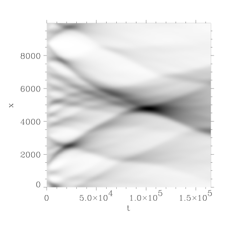
FIG. 3.: Time evolution of the particle density. Dark regions indicate high density.

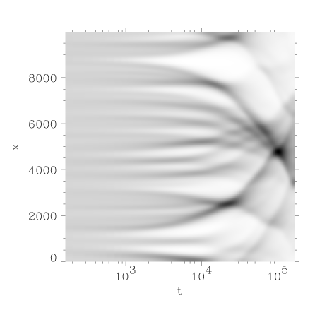
FIG. 4.: The same as fig. 3 on a logarithmic time scale

As is well known, inelastic particles without internal structure tend to cluster in one dimension. This clustering leads to a break down (inelastic collapse) of the system if $\epsilon$ is constant and less than a critical value that depends solely on the number of particles. In our model particles have internal degrees of freedom and the translational energy is not completely lost in a collision but is stored in the internal vibrations and can be transferred back to the translational motion. Due to the properties of $p_{\beta}(\epsilon)$ (see section II B), the probability for this to happen gets larger as the translational energy decreases. Therefore clusters do form but dissolve after a while and no inelastic collapse takes place.

We start again from a spatially homogeneous distribution of particles and analyse evolving spatial structures with help of a coarse grained density $\rho$. We divide the total length of the ring into a hundred bins and count the number of particles in each bin. The coarse grained density is defined as the actual number of particles in each bin divided by the average.

The time evolution of $\rho$ is shown in fig. 3 on a linear time scale and in fig. 4 on a logarithmic time scale. Several phases in the cooling process can be identified. First, the particles start to form clusters and voids as they lose kinetic energy in collisions (initially, when $T_{B}$ is small compared to the translational energy, the coefficient of restitution is always close to $\gamma$). After these clusters have formed, one observes collisions of clusters, forming larger clusters. Simultaneously the dissolution of clusters starts to set in, the remains being sent outwards to join neighbouring clusters. The biggest clusters and voids are seen to survive for times of order $10^{4}$. This complex interaction of forming and dissolving clusters continues with a clear tendency to form fewer and larger clusters. Finally these large clusters dissolve to establish the equilibrium state, i. e. equipartition among all degrees of freedom.

For 10000 particles it takes a time of order $10^{5}$ until the cooling dynamics is finished and the equilibrium state for the larger system is reached, whereas for 50 particles it takes only a time of order $10^{3}$ (see fig. 1). The equilibrium state is reached only after the formation and dissolution of essentially one final large cluster. In a smaller system the end of the cascade of clusters of increasing size is reached earlier, simply because there are fewer particles.

Phase space

The complete information about the state of the system at time $t$ is contained in a phase space plot, as shown in fig. 5. Within a cluster of particles we expect frequent collisions and hence an effective transfer of kinetic energy to internal vibrations. Frequently regions of high average density are characterized by particle velocities centered around zero. However, we also observe clusters with an average nonzero velocity, resulting at a later time in collisions of clusters. One such collision of two clusters can be traced in fig. 5 around $x\sim 2500$. In fig 5a (a snapshot taken at $t=14000$) one observes two clusters both with nonzero average velocity moving towards each other, wheras in fig 5b (taken at $t=20000$) the clusters have collided and formed a larger one.

(a)

(b)

FIG. 5.: Phase space plot of the system at two different times.

We also see around $x\sim 1000$ the occurrence of a stripe-shaped fluctuation in the phase-space plot. This type of fluctuation has already been observed and discussed by McNamara and Young [4] and Sela and Goldhirsch [5]. It gives rise to the formation of clusters out of an initially homogeneous region. Thus figure 5 shows that the dynamics of our system are indeed rather complex as formation, movement, interaction and dissolution of clusters all happen simultaneously.

Local kinetic energy

It is interesting to see how the kinetic energy is spatially distributed. We define a coarse grained kinetic energy density similar to the coarse grained density by summing the kinetic energies of all particles inside a bin and dividing by the number of particles in the bin.

One might be tempted to conjecture that the local kinetic energy is in some way correlated to the clustering because most collisions occur within the clusters. Fig. 6 (as an example) reveals, however, that this is generally not the case: although the kinetic energy shows some structure there is no visible correlation to the density, not even in a state as the one shown in fig. 6, where all the particles are extremely clustered. Fig. 6 is a snapshot of the system at time $t=100343$ (cf. figs. 3 and 4).

FIG. 6.: Comparison of the local kinetic energy (dashed line) and particle density (solid line).

Velocity distribution

In the cooling stage, the system is still far from equilibrium, so that the velocity distribution of the particles is not expected to be a Maxwell distribution. It is therefore interesting to test what kind of distribution the velocities really follow.

Data analysis shows that the velocity distribution of ${\it all}$ particles is indeed not a Gaussian distribution (see fig. 7). There are relatively large deviations especially near the maximum of the curve. If one restricts the data analysis to only those particles inside a single cluster, however, one finds that the velocity distribution of these is to a much better degree gaussian, considering that there are only about 1/10th of the total number of particles in the cluster. This can be well understood because there are many collisions between particles inside a cluster and thus a local equilibrium is reached, resulting in a Maxwellian distribution. On the other hand the velocity distribution of all particles reflects the velocity distribution of the clusters. As long as the complicated process of forming and dissolution of clusters is underway, the clusters are naturally

FIG. 7.: Velocity distribution of all particles (circles) and the particles inside one particular cluster (triangles) at time $t=14000$. The cluster chosen for this curve is centered around $x=2000$ (cf. figs. 3, 4 and 5a)

far away from equilibrium. This leads to the observed deviations from the gaussian curve.

Since our system is far away from the quasielastic limit, we see quite a different velocity distribution than MacNamara and Young [4], who simulated a one dimensional system of quasielastic particles. They observed a bimodal velocity distribution because the particles tend to concentrate on the upper and lower edges of a band in a phase space plot similar to fig. 5. In our simulation, the situation is much more complex because of the formation of many clusters, each with its own velocity distribution.

Correlation function

The inelasticity of collisions leads to a clustering of particles, as can be seen in figs. 3 and 4. Williams [18] has described a one dimensional system of individually heated granular particles. He found that the pair correlation function, defined by $g(x)=\frac{1}{N-1}\sum_{i\neq j}\delta(x-|x_{i}-x_{j}|)$ of the system in the steady state approximately follows a power law. Here, we observe quite a different behaviour of the correlation function (see fig. 8).

FIG. 8.: The pair correlation function $g(x)$ of the system at $t=14000$.

Instead of showing a divergence at zero separation, it levels off to a plateau. The explanation for such a different behaviour lies in the mechanism of heating: When the particles are heated individually, i. e. when they are driven by a random force, they will half of the time be kicked back in the direction of the particle that they last collided with. Thus there is some additional tendency for the particles to stick together. In our model, however, the particles will only change their velocity when they collide, thus favouring larger distances.

It should be noted that the correlation function in fig. 8 is not that of the steady state of our system but a snapshot taken during the cooling process. The steady state of our model is trivial, implying a constant correlation function, $g(x)\equiv 1$.

IV Damped internal modes

So far we have considered a conservative system, i. e. the total energy of translational motion and internal vibrations is conserved. Such a model gives rise to a stationary equilibrium state in which equipartition among all degrees of freedom holds, so that the translational momenta are of order $O(1/\sqrt{N_{mod}})$. To model granular media, one should take into account additional dissipative mechanisms, which result in a decrease of the total energy so that the particles are truly at rest in the stationary state. One such mechanism is black body radiation.

A simple way to model this effect is to let the bath temperature of each particle decay in time. Hence we suggest the following modification of the algorithm of sec. II C. Inbetween collisions the particles move freely and their bath temperature decreases according to a simple exponential decay

$$T_{B}^{i}(t)=T_{B}^{i}(t_{i})\exp{(-(t-t_{i})\nu)}\quad\mbox{for}\quad t>t_{i}$$ (36)

Here $t_{i}$ denotes the instant of time when the last collision of particle $i$ took place. The same decay frequency $\nu$ is used for all particles. The updating of relative velocities and bath temperatures in a collision is unchanged as compared to sec. II C.

We expect that the effect of such a dissipative mechanism will strongly depend on the frequency of collisions as compared to $\nu$. If collisions are rather infrequent, then the decay will be effective and the bath of the particles will cool down in between collisions. The resulting dynamics should resemble the deterministic case and hence one should observe a strong increase in the collision frequency, because the system is developing towards inelastic collapse. When this happens, the collision frequency becomes comparable or even smaller than the decay rate $\nu$. In that case the internal modes can no longer relax in between collisions. In the limit of very high collision frequencies the bath temperatures are effectively non-decaying, so that one recovers the algorithm of sec. II C without any dissipation. Hence we expect to see the system develop towards inelastic collapse with a strong increase in collision frequency, followed by a period of time where the collision frequency levels off.

These expectations are confirmed by numerical simulations of once again 10000 particles with $\nu=0.01$. In fig. 9 we show the total number of collisions as a function of time. One clearly observes rather sharp steps followed by smoother regions, as explained above. In fig. 10 we show the decrease in total kinetic energy as a function of time. Steep regions of the collision frequency correspond to steep regions in the energy plot because the frequent collisions among clustered particles draw much energy out of the system.

FIG. 9.: Number of collisions as a function of time for the dissipative system.

FIG. 10.: Decrease of the total kinetic energy as a function of time for the dissipative system.

An important question is the following: What is the stationary state of the system with dissipation and how long does the system need to relax to the stationary state? The final state should be one big cluster, with all particles at rest. As explained above, the dynamics with dissipation resemble the dynamics of a deterministic system as long as no inelastic collapse is at hand. For this reason it can be expected that the kinetic energy on the average follows the mean field result $E\sim t^{-2}$, occasionally disrupted by the occurence of a cluster, which is however quickly dissolved. Simulations show that this behaviour can indeed be observed, see fig. 11. Since the above mentioned scaling law never permits the energy to become exactly 0 in a finite time, the stationary state (which has energy 0) can also never be reached in finite time.

FIG. 11.: Decrease of the kinetic energy as a function of time for 50 dissipative particles. The dashed line shows the $E\sim t^{-2}$ relation.

V Conclusion

We have presented the results of simulations performed on a recently developed model for a one dimensional granular medium. The model allows for an algorithm which is a hybrid of Monte Carlo and Event Driven and which avoids the inelastic collapse. Thus, we have been able to perform long simulations on a large system far away from the quasielastic limit. The model in its simplest form conserves energy: translational energy can be transferred to internal vibrational modes of the particles and vice versa. Starting from a state with no internal modes excited, there is a long cooling regime, extending over several orders of magnitude in time, before the stationary state, characterized by equipartition of energy, is reached. The decrease of kinetic energy during this cooling stage shows considerable deviations from the mean field result $E_{kin}\sim t^{-2}$. We have also observed a complex process of cluster forming, movement, interaction and dissolution. Inside the clusters we find that the particles are close to local equilibrium, which is indicated by the fact that a Maxwellian velocity distribution with in general nonzero mean velocity holds for particles in the cluster.

The model has been extended to include net dissipation of energy by exponential damping of the internal modes. In this case, the algorithm still shows no inelastic collapse. On the average, the decrease of the kinetic energy follows the mean field result but with considerable fluctuations due to the complex cluster dynamics which are still a feature of the model with energy dissipation.

Thus our model, which is based on a microscopic mechanism for the loss of translational energy during collisions, is well suited as a starting point for simulation and theoretical description of one dimensional granular media. Unlike many other models, it makes use of an exact treatment of the collision dynamics of the colliding rods and hence offers a possible intuitive way of understanding the precise manner in which translational energy is removed from a granular system. Future work will use this model to investigate the properties of driven granular assemblies. In our model a specific mechanism – transfer of translational energy to internal vibrations – has been analysed to develop a microscopic basis for an effective coefficient of restitution. One may wonder which of our results depend on the particular mechanism. To study this question, we are presently investigating distributions $p_{\beta}(\epsilon)$ which are only restricted by detailed balance and not derived from a microscopic model. One may also try to extend our analysis to higher dimensional objects like disks or spheres. In the simplest geometry these objects are colliding in a one dimensional tube, so that no tangential forces like coulomb friction have to be considered. Our microscopic model is easily generalized to this case and allows for investigating how effectively energy of translation is transferred to elastic vibrations [20]. The frequently used quasistatic approximation of Hertz implies no energy transfer at all.

REFERENCES

- [1] G. Giese and A. Zippelius, Phys. Rev. E54, 4828 (1996). A short summary of the results has been published in [2].
- [2] G. Giese in D. E. Wolf, M. Schreckenberg, and A. Bachem (eds.): Traffic and Granular Flow (World Scientific, Singapore 1996), p. 335.
- [3] B. Bernu and R. Mazighi, J. Phys. A 23, 5745 (1990);
- [4] S. McNamara and W. R. Young, Phys. Fluids 4, 496 (1992) and S. McNamara and W. R. Young, Phys. Fluids 5, 34 (1993).
- [5] N. Sela and I. Goldhirsch, Phys. Fluids 7, 507 (1995).
- [6] E. Clement, S. Luding, A. Blumen, J. Rajchenbach and J. Duran, Intern. J. Mod. Phys. B7, 1807 (1993);
- [7] S. Luding, E. Clement, A. Blumen, J. Rajchenbach, and J. Duran, Phys. Rev. E49, 1634 (1994).
- [8] J. M. Luck and Anita Mehta, Phys. Rev. E48, 3988 (1993).
- [9] A. P. Hatzes, F. G. Bridges, and D. N. C. Lin, Mon. Not. R. astr. Soc. 231, 1091 (1988); K. D. Supulver, F. G. Bridges, and D. N. C. Lin, Icarus 113, 188 (1995)
- [10] H. Hertz, J. Reine Angew. Math. 92, 156 (1996).
- [11] Th. Poeschl, Z. Phys. 46, 142 (1928).
- [12] Y.- H. Pao, J. Appl. Phys. 26, 1083 (1955).
- [13] N. V. Brilliantov, F. Spahn, J. M. Hertzsch, and T. Poeschel, Phys. Rev. E53, 5382 (1996); J. M. Hertzsch, F. Spahn, and N. V. Brilliantov, J. Phys. (Paris) II, 5, 1725 (1995).
- [14] J. Hertzsch, H. Scholl, F. Spahn, and I. Katzorke, Astron. & Astrophys. 320, 319 (1997); F. Spahn, U. Schwarz, and J. Kurths, Phys. Rev. Lett. 78, 1596 (1997).
- [15] For a pedagogical discussion of the wave theory of elastic rods see e.g. D. Auerbach, Am. J. Phys. 62, 522 (1994).
- [16] see e.g. P. E. Kloeden and E. Platen, Numerical solution of stochastic differential equations (Springer, Berlin, 1992), p. 42.
- [17] T. Aspelmeier and A. Zippelius, to be published.
- [18] D. R. M. Williams, Physica A233, 718 (1996).
- [19] Y. Du, H. Li, and L. P. Kadanoff, Phys. Rev. Lett. 74, 1268 (1995); R. Mazighi, B. Bernu, and F. Delyon,Phys. Rev. E50, 4551 (1994);
- [20] F. Gerl, private communication