Pairing correlation in the two- and three-leg Hubbard ladders
— Renormalization and quantum Monte Carlo studies

Abstract

In order to shed light whether the ‘even-odd conjecture’ (even numbers of legs will superconduct accompanied by a spin gap while odd ones do not) for correlated electrons in ladder systems, the pairing correlation is studied for the Hubbard model on a two- and three-leg ladders. We have employed both the weak-coupling renormalization group and the quantum Monte Carlo (QMC) method for strong interactions. For the two-leg Hubbard ladder, a systematic QMC (with a controlled level spacings) has detected an enhanced pairing correlation, which is consistent with the weak-coupling prediction. We also calculate the correlation functions in the three-leg Hubbard ladder and show that the weak-coupling study predicts the dominant superconductivity, which refutes the naive even-odd conjecture. A crucial point is a spin gap for only some of the multiple spin modes is enough to make the ladder superconduct with a pairing symmetry (d-like here) compatible with the gapped mode. A QMC study for the three-leg ladder endorses the enhanced pairing correlation.

I Introduction

Over the past several years, strongly correlated electron systems with quasi-one-dimensional (1D) ladder structures have received much attention theoretically and experimentally. Experimental studies have received much impetus, since cuprate compounds containing such structures have been fabricated recently.[2]

The idea was inspired theoretically in 1986, when Schulz[3] conjectured the following. If we consider a gas of repulsively interacting electrons on a ladder, the undoped system will be a Mott insulator, so that we may consider the system as an $S=1/2$ antiferromagnetic (AF) Heisenberg magnet on a ladder. Then an AF ladder with $N$-legs should be similar to a AF $S=N/2$ single chain, which is exactly Haldane’s system.[3, 4, 5] For the latter Haldane’s conjecture predicts that the spin excitation should be gapless for a half-odd-integer spin ($N$: odd) or gapful for an integer spin ($N$: even). If the situation would be similar in ladders, a ladder having an even number of legs will have a spin gap, which should indicate that the ground state is a ‘spin liquid’ where the quantum fluctuation is so large that spins cannot order. On the other hand an odd number of legs will have gapless spin excitations, which should indicate that the ground state has an AF order. The presence of a spin gap in the former case may be a good news for superconductivity, since, there is a body of ideas dictating that a way to obtain superconductivity is to carrier-dope a system that has a spin gap in the course of the study of high-$T_{C}$ superconductivity. Such a scenario has been put forward by Rice et al.[6]

As far as the spin gap is concerned, both theoretical[7, 8, 9, 10, 11] and experimental[12, 13, 14, 15] studies on the undoped-ladder systems have indeed supported the conjecture.

The spin-gap conjecture has recently been confirmed experimentally[12, 13, 14]. Namely, a class of cuprates, Sr_n-1Cu_nO_2n-1, has $n$-leg ladders on a CuO₂ plane, and the two-leg ladders in SrCu₂O₃ exhibit a spin-liquid behavior characteristic of finite spin-correlation lengths, while the three-leg ladders in Sr₂Cu₃O₅ have an AF behavior.

Rice et al. have further conjectured for doped systems that an even-numbered ladder should have a dominant interchain d-wave-like pairing correlation as expected from the persistent spin gap away from half-filling.[6] The conjecture is partly based on an exact diagonalization study for finite systems for a two-leg $t-J$ ladder by Dagotto et al.[7] This was then followed by analytical[16] and numerical[10, 17, 18, 19, 20, 21] works on the doped $t-J$ ladder, which support the dominant pairing correlation in a certain region. In the phase diagram, the region for the dominant pairing correlation appears at lower values of exchange coupling $J$ than in the case of a single chain. Experimentally Uehara et al.[22] have recently observed superconductivity in a two-leg ladder material Sr_0.4Ca_13.6Cu₂₄O_41.84 under high pressures.

The Hubbard models on ladders are also of interest, since the Hubbard model may be regarded as an effective model for cuprates (Fig.1). Since there is no exact solution for the Hubbard ladder, a most reliable analytical method at present is the weak-coupling theory,[23, 24] which, in the continuum limit, linearizes the band structure around the Fermi points to treat the interaction with a perturbative renormalization group.

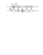
FIG. 1.: Two-leg Hubbard ladder model; $t(t_{\perp})$ and $U$ are the intrachain(interchain) hopping and the on-site interaction, respectively.

The weak-coupling theory has been applied to the two-leg Hubbard ladder. [27, 28, 30, 31] At half-filling, the system reduces to a spin-liquid insulator having both charge and spin gaps[27] with a finite SDW correlation length. Although one might expect that the Hubbard ladder would not exhibit a sizeable spin gap at half-filling unlike the $t-J$ ladder, the spin gap for the Hubbard model estimated with DMRG by Noack et al.[32, 33] is as large as 0.13$t(\sim 400$K for $t\sim 0.3$eV for $U=8t$ with $t_{\perp}=t$, which should correspond to the cuprates). The magnitude of the spin gap is comparable with the spin gap ($\sim$ 400K) experimentally estimated from the magnitude of susceptibility for SrCu₂O₃.

When the carrier is doped, the weak-coupling theory supports the dominance of the pairing correlation whose symmetry is the same as that of the $t-J$ ladder. The relevant scattering processes at the fixed point in the renormalization flow are the pair-tunneling process across the bonding and the anti-bonding bands (Fig.2), and the backward-scattering process within each band. The importance of the pair-tunneling across the two bands (which exists in two or larger numbers of legs) for the dominance of pairing correlation in the two-leg Hubbard ladder is reminiscent of the Suhl-Kondo mechanism, that was proposed back in the 1950’s for superconductivity in the transition metals with two (s- and d-like) bands.[34, 35] Muttalib and Emery have shown another example of the pair-tunneling mechanism for superconductivity with purely repulsive interactions.[36] More recently, the superconductivity in $t-t^{\prime}-U$ model, which may be relevant for the chains that alternate with the ladder layers in the cuprates[29], has also been studied analytically[37] and numerically[38] as a 1D ladder-like system.

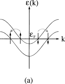
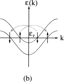
FIG. 2.: Relevant pair-tunneling processes in two-leg Hubbard ladder; Fig.(a) (Fig.(b)) is the forward (backward) type pair-tunneling process.

The properties of the weak-coupling Hubbard ladder are similar to those of the $t-J$ ladder for the regime where the pairing correlation is dominant: in addition to the existence of the spin gap, the duality relation[30, 31], which suggests that the exponent for the pairing correlation $(\sim r^{1/(2K_{\rho}}))$ should be reciprocal to that for the $4k_{F}$ CDW correlation $(\sim r^{(2K_{\rho}}))$, holds in both the weak-coupling Hubbard ladder and the $t-J$ ladder.[18, 19, 21] Here $K_{\rho}$ is the critical exponent for the gapless charge mode, which tends to unity in the weak-coupling limit. The similarity may come from the form of the excitation gaps in the bosonization description. In both $t-J$ and Hubbard ladders[30], the only gapless mode is a charge mode with none of the spin modes being gapless (‘C1S0’ phase in the language of the weak-coupling theory[27]).

However, there is a serious reservation for the weak-coupling theory. First, whether the model in the continuous limit is indeed equivalent to the lattice model is not obvious. More serious is the problem that the perturbational renormalization group is guaranteed to be valid only for an infinitesimally small interaction strengths in principle. Specifically, when there is a gap in the excitation, the renormalization flows into a strong-coupling regime, so that the perturbation theory may well break down even for small interaction strengths. A way to check the reliability of the weak-coupling theory is to treat finite systems with larger $U$ with numerical calculations such as exact diagonalization, density-matrix renormalization group (DMRG), or quantum Monte Carlo (QMC) methods[25, 26]. Numerical calculations, on the other hand, have drawbacks due to finite-size effects. Thus the weak-coupling theory and the numerical methods should be considered as being complementary.

Specifically, the dominance of the pairing correlation is indeed a subtle problem in numerical calculations. Existing numerical results[32, 33, 39, 40, 47] do appear to be controversial, where some of the results are inconsistent with the weak-coupling prediction as detailed in Sec.II.

If we ignore these controversies, most of the existing theories support the dominance of the pairing correlation in the doped two-leg ladders. Then, an even more important unresolved problem for superconductivity in the doped ladders is the ‘even-odd’ conjecture. One can naively expect that the absence of spin gaps in odd-numbered legs will signify an absence of dominating pairing correlation, which will end up with an ‘even-odd conjecture for superconductivity’. Indeed there has not been works looking into the pairing correlation functions for the three-leg ladder, which is the simplest realization of odd-numbered legs. White et al.[41] have studied two holes doped in the $t-J$ ladders at half-filling to find that two holes are bound in even-numbered (two or four) legs, while they are not in odd-numbered (three or five) legs, but (i)the existence of a binding energy for two carriers is not directly connected with the occurrence of superconductivity, and (ii)the $t$-$J$ model and the Hubbard model may exhibit different behaviors.

Thus the second purpose of the present paper is to study the pairing correlation in Hubbard ladder models with three legs as compared with the two-leg case.

The organization of the present paper is as follows. We first study the two-leg Hubbard ladder model[42] having intermediate interaction strengths with the QMC method in Sec.II. A new ingredient in this study is that we pay a special attention to the non-interacting ($U=0$) single-particle energy levels which are discrete in finite systems. We have found that if we make the levels on the two bands aligned (within an energy that is smaller than the spin gap) to mimic the thermodynamic limit, the weak-coupling result (an enhanced pairing correlation in the present case) is in fact reproduced for intermediate $U$. Further we check the effects of the inter- and intra-band Umklapp-scattering processes, which are expected to be present at the special band fillings from the weak-coupling theory[27].

In Sec.III we study three(odd)-leg Hubbard ladder model (Fig.3) with the weak-coupling theory[43] using the enumeration of gapless modes by Arrigoni.[44] The system has one gapless spin mode and two gapful spin modes. Thus the gapful and the gapless spin modes coexist. The existence of the gapful modes is a result of the relevant interband pair-tunneling process across the top and the bottom bands (Fig.4). We find that this gives rise to a dominant pairing correlation across the central and the edge chains reflecting the gapful spin modes, which coexists with the subdominant but power-law decaying SDW correlation reflecting the gapless spin mode. Thus the Suhl-Kondo-like mechanism for superconductivity exists not only in two-leg systems but also in a three(odd)-leg system as well, while the SDW correlation also survives as expected. Schulz[45] also found similar results independently.

FIG. 3.: Three-leg Hubbard ladder model; $t(t_{\perp})$ and $U$ are the intrachain (interchain) hopping and the on-site interaction, respectively.

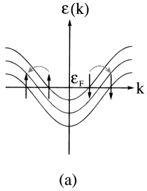
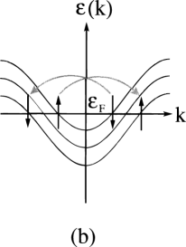
FIG. 4.: Relevant pair-tunneling processes in the three-leg Hubbard ladder; Fig.(a) (Fig.(b)) is the forward (backward) type pair-tunneling process.

We then study the three-leg Hubbard ladder model in Sec.IV with a QMC calculation[46] as in the two-leg case. The technique to detect the enhanced pairing correlation in the two-leg case is also valid in the three-leg case. We found that the enhancement of the pairing correlation persists for the intermediate interaction strengths. We also study the effects of the Umklapp processes at special band fillings as in the two-leg case.

The above numerical calculations for two or three legs are performed in a condition that the one-body energy levels are close to each other. We believe this condition mimics the situation in the thermodynamic limit. In Sec.V, a circumstantial evidence for this is given by a QMC calculation of the pairing correlation in the 1D attractive Hubbard model, which can be exactly solved with the Bethe Ansatz[49], so that the exact asymptotic form of the correlation functions and the values of the spin gap are known at arbitrary values of parameters.

II Quantum Monte Carlo study of the pairing correlation in the two-leg Hubbard ladder

In this section, we study the pairing correlation for the two-leg Hubbard ladder (Fig.1). The Hamiltonian of the two-leg Hubbard ladder is given in standard notations as

$${\cal H} = -t\sum_{\alpha i\sigma}(c_{\alpha i\sigma}^{\dagger}c_{\alpha i+1\sigma}+{\rm h.c.})$$ (2)

$$-t_{\perp}\sum_{i\sigma}(c_{1,i\sigma}^{\dagger}c_{2,i\sigma}+{\rm h.c.})+U\sum_{\alpha i}n_{\alpha i\uparrow}n_{\alpha i\downarrow},$$

where $\alpha(=1,2)$ specifies the chains and $t(t_{\perp})$ is the intra(inter)-chain hopping.

From an analytical point of view, if the system is free from Umklapp processes, the weak-coupling theory with the bosonization combined with the renormalization-group techniques [27, 28, 30, 31] has indeed shown that the the two-leg Hubbard ladder has a spin gap and that the correlation function of the interchain d-wave-like pairing order parameter, $O_{i}=(c_{1i\uparrow}c_{2i\downarrow}-c_{1i\downarrow}c_{2i\uparrow})/\sqrt{2}$, decays as $\sim r^{-1/(2K_{\rho})}$ as a result of the relevant pair-tunneling process (Fig.2), where $K_{\rho}$ is the critical exponent for the total-charge-density mode being only gapless and tends to unity in the weak-coupling limit.

Since SDW and $2k_{F}$ CDW correlations have to decay exponentially in the presence of a spin gap in a two-leg ladder, the only phase competing with pairing correlation will be $4k_{F}$ CDW correlation, which should decay as $r^{-2K_{\rho}}$. Hence the pairing correlation dominates over all the others if $K_{\rho}>1/2$. In numerical calculations, however, the dominance of the pairing correlation in the Hubbard ladder appears to be a subtle problem. Namely, a DMRG study by Noack et al. for the doped Hubbard ladder with $n=0.875$, $U/t=8$, and $t_{\perp}=t$ shows no enhancement of the pairing correlation over the $U=0$ result[32, 33], while they do find an enhancement at $t_{\perp}=1.5t$[33, 47]. Asai performed a quantum Monte Carlo (QMC) calculation for a 36 rungs ladder with $n=0.833$, $U/t=2$ and $t_{\perp}=1.5t$[40], in which no enhancement of the pairing correlation was found. On the other hand, Yamaji et al. have found an enhancement for the values of the parameters when the lowest anti-bonding band levels for $U=0$ approach the highest occupied bonding band levels, although their results have not been conclusive due to the small system sizes ($\leq 6$ rungs).[39] Thus, the existing analytical and numerical results appear to be controversial in the two-leg Hubbard ladder.

Another point is that the above results are obtained away from special fillings where the Umklapp-scattering processes are irrelevant. Recently, Balents and Fisher[27] proposed a weak-coupling phase diagram (Fig.5) which displays the numbers of the gapless spin and charge phases on the $t_{\perp}-n$ plane (where $n$ is the band filling). The effects of the Umklapp processes are also discussed there. At half-filling the interband Umklapp processes become relevant resulting in a spin-liquid insulator in which the pairing correlation decays exponentially. In addition, the intraband Umklapp process within the bonding band becomes relevant resulting in a gap in one charge mode in a certain parameter region where the bonding band is reduced to a half-filled band. This phase is called ‘C1S2’ phase because there are one gapless and two gapfull charge modes, while the phase at half-filling is called ‘C0S0’ phase because there is no gapless phase. We can expect that the pairing correlation decays exponentially or is at least suppressed reflecting the existence of the charge gap, although the direct calculation of the pairing correlation has not been done. Thus we also study the effects of the Umklapp processes in this section, keeping in mind the above weak-coupling results.

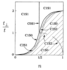
FIG. 5.: Phase diagram in the weak-coupling limit ($U\rightarrow 0$) given in ref. [39]; the numbers of the gapless charge and spin modes ($x$ and $y$, respectively) are denoted as C$x$S$y$ and $n$ is the band filling. In the dark region both of the two bands cross the Fermi level.

In the remaining of this section, we perform an extensive projector QMC calculation[25, 26] to investigate the ground state correlation function $P(r)\equiv\langle O_{i+r}^{\dagger}O_{i}\rangle$ for the pairing in the Hubbard ladder[42] with $t_{\perp}\sim t$, especially in order to clarify the origin of the discrepancies among the existing results. We conclude that the discreteness of energy levels in finite systems affects the pairing correlation enormously.

The details of the QMC calculation are the following. We assumed the the periodic boundary conditions along the chain direction, $c_{N+1}\equiv c_{1}$ (where $N$ labels the rungs) and took the non-interacting Fermi sea as the trial state The projection imaginary time $\tau$ was taken to be $\sim 60/t$. We need such a large $\tau$ to ensure the convergence of especially the long-range part of the pairing correlation. This sharply contrasts with the situation for single chains, where $\tau\sim 20/t$ suffices for the same sample length as considered here. The large value of $\tau$, along with a large on-site repulsion $U$, makes the negative-sign problem serious, so that the calculation is feasible for $U/t\leq 2$. In the Trotter decomposition, the imaginary time increment $[\tau/$(number of Trotter slices)] is taken to be $\leq 0.1$. We have concentrated on band fillings for which the closed-shell condition (no degeneracy in the non-interacting Fermi sea) is met. We set $t=1$ in the remaining of this section.

In the beginning we show in Fig.6 the result for $P(r)$ for $t_{\perp}=0.98$ and $t_{\perp}=1.03$ with $U=1$ and the band filling $n=0.867=52$ electrons/ (30 rungs $\times$ 2 legs). The $U=0$ result (dashed line) for these two values of $t_{\perp}$ are identical because the Fermi sea remains unchanged. However, if we turn on $U$, the 5% change in the $t_{\perp}=0.98\rightarrow 1.03$ is enough to cause a dramatic change in the pairing correlation: for $t_{\perp}=0.98$ the correlation has a large enhancement over the $U=0$ result at large distances, while the enhancement is not seen for $t_{\perp}=1.03$.

FIG. 6.: Pairing correlation function, $P(r)$, plotted against the real-space distance $r$ in a 30 rungs Hubbard ladder having 52 electrons for $U=1$ with $t_{\perp}=0.98$ ($\Box$) and $t_{\perp}=1.03$ ($\diamond$ ). The dashed line is the noninteracting result for the same system size, while the straight dotted line represents $\propto 1/r^{2}$. The solid line is a fit to the $U=1$ result with $t_{\perp}=0.98$ (see text).

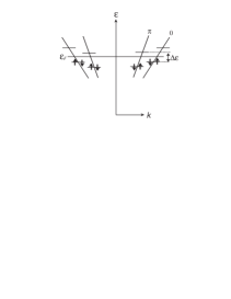
FIG. 7.: Schematic image of the discrete energy levels of both bonding ($0$) and anti-bonding ($\pi$) bands for $U=0$.

In fact we have deliberately chosen these values to control the alignment of the discrete energy levels at $U=0$. Namely, when $t_{\perp}=0.98$, the single-electron energy levels of the bonding and anti-bonding bands for $U=0$ lie close to each other around the Fermi level with the level offset ($\Delta\varepsilon$ in Fig.7) being as small as 0.004, while they are staggered for $t_{\perp}=1.03$ with the level offset of 0.1. On the other hand, the size of the spin gap is known to be around $0.05$ for $U=8$,[47, 33] and is expected to be of the same order of magnitude or smaller for smaller values of $U$. The present result then suggests that if the level offset $\Delta\varepsilon$ is too large compared to the spin gap (which should be O(0.01) for $U\sim t$,[33]) the enhancement of the pairing correlation is smeared. By contrast, for a small enough $\Delta\varepsilon$, by which an infinite system is mimicked, the enhancement is indeed detected in agreement with the weak-coupling theory, in which the spin gap is assumed to be infinitely large at the fixed point of the renormalization flow. Similar situation is also found in the case of a QMC study of the pairing correlation in the $t-t^{\prime}-U$ model.[38]

Our result is reminiscent of those obtained by Yamaji et al.,[39] who found an enhancement of the pairing correlation in a restricted parameter regime where the lowest anti-bonding levels approach the highest occupied bonding levels. They conclude that the pairing correlation is dominant when the anti-bonding band ‘slightly touches’ the Fermi level. However, our result in Fig.6 is obtained for the band filling for which no less than seven out of 30 anti-bonding levels are occupied at $U=0$. Hence the enhancement of the pairing correlation is seen to be not restricted to the situation where the anti-bonding band edge touches the Fermi level.

However, one might consider that the enhancement of the pairing correlation in such a condition for the one-body energy levels should be rather due to finite size effects, although we believe the condition is generally relevant for bulk systems. To clarify this point, we will further give a circumstantial evidence to justify that the condition for the one-body energy levels is relevant for bulk systems by a QMC study for 1D attractive Hubbard model in Sec.V.

Now, let us more closely look into the form of $P(r)$ for $t_{\perp}=0.98$. It is difficult to determine the exponent from results for finite systems, but here we attempt to fit the data by assuming a trial function expected from the weak-coupling theory. Namely, we have fitted the data with the form,

$$P(r) = \frac{1}{4\pi^{2}}\sum_{d=\pm}\{cr_{d}^{-1/2}$$ (4)

$$+[(2-c)-\cos(2k_{F}^{0}r_{d})-\cos(2k_{F}^{\pi}r_{d})]r_{d}^{-2}\}$$

with the least-square fit (by taking logarithm of the data). Because of the periodic boundary condition, we have to consider contributions from both ways around, so there are two distances between the $0$-th and the $r$-th rung, i.e, $r_{+}=r$ and $r_{-}=N-r$. The periods of the cosine terms are assumed to be the non-interacting Fermi wave numbers of the bonding and the anti-bonding bands in analogy with the single-chain case.

The overall decay should be $1/r^{2}$ as in the pure 1D case in the weak-coupling limit. We have assumed the form $c/r^{1/2}$ as the dominant part of the correlation at large distances because this is what is expected in the weak-coupling theory. Here $c$ is the only fitting parameter in the above trial function. A finite $U\sim 1$ may give some correction, but the result (solid line in Fig.6) fits to the numerical result surprisingly accurately with a best-fit $c=0.10$. If we least-square fit the exponent itself as $1/r^{\alpha}$, we have $\alpha<0.7$ with a similar accuracy. Thus a finite $U$ may change $\alpha$, but $\alpha>1$ may be excluded. To fit the short-range part of the data, a non-oscillating $(2-c)/r^{2}$ term is required, which is not present in the weak-coupling theory. We believe that this is because the weak-coupling theory only concerns with the asymptotic form of the correlation functions.

In Fig.7, we show a result for a larger system size (42 rungs) for a slightly different electron density, $n=0.905$ with 76 electrons and $t_{\perp}=0.99$. We have again an excellent fit with $c=0.07$ this time.

FIG. 8.: Plot similar to that in Fig.6 for a 42 rungs system having 76 electrons with $t_{\perp}=0.99$.

In Fig.8, we display the result for a larger $U=2$. We again have a long-ranged $P(r)$ at large distances, although $P(r)$ is slightly reduced from the result for $U=1$. This is consistent with the weak-coupling theory, in which $K_{\rho}$ is a decreasing function of $U$ so that after the spin gap opens for $U>0$, the pairing correlation decays faster for larger values of $U$.

FIG. 9.: Plot similar to that in Fig.6 for $U=2$.

Now we explore the effects of the Umklapp processes. For that purpose we concentrate on the filling dependence for a fixed interaction $U=2$. We have tuned the value of $t_{\perp}$ to ensure that the level offset $(\Delta\varepsilon)$ at the Fermi level is as small as O($0.01$) for $U=0$. In this way, we can single out the effects of the Umklapp processes from those due to large values of $\Delta\varepsilon$. If we first look at the half-filling (Fig.10), the decaying form is essentially similar to the $U=0$ result. At half-filling, the interband Umklapp processes emerge and, according to the weak-coupling theory, open a charge gap, which results in an exponential decay of the pairing correlation. (We should note that there are two kinds of charge gaps. The one, which is produced by the pair-tunneling processes, causes the long range order of the Josephson phase resulting in the enhancement of the pairing correlation, while the other, which is produced by the Umklapp processes, causes the long range order of the phase of the CDW resulting in the suppression of the pairing correlation)

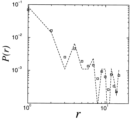
FIG. 10.: Pairing correlation $P(r)$ ($\Box$) against $r$ for a 30 rungs system for $U=2$ with $t_{\perp}=0.99$ and 60 electrons (half-filled). The dashed line represents the non-interacting result.

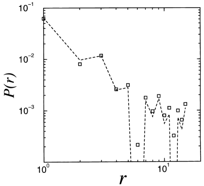
FIG. 11.: Pairing correlation $P(r)$ ($\Box$) against $r$ for a 30 rungs system for $U=2$ with $t_{\perp}=1.01$ and 40 electrons (half-filled bonding band). The dashed line represents the non-interacting result.

It is difficult to tell from our data whether $P(r)$ decays exponentially. This is probably due to the smallness of the charge gap. In fact, the DMRG study by Noack et al.[32, 33] have detected an exponential decay for larger values of $U$, for which a larger charge gap is expected.

When $n$ is decreased down to 0.667 (Fig.11), we again observe an absence of enhancement in $P(r)$. This is again consistent with the weak-coupling theory[27]: for this band filling, the number of electrons in the bonding band coincides with $N(=30)$ at $U=0$, i.e., the bonding band is half-filled. This will then give rise to intraband Umklapp processes within the bonding band resulting in the ‘C1S2’ phase as discussed in Section 2.1. The spin gap is destroyed and the singlet-pair of electrons or holes are prevented from forming, so that the pairing correlation will no longer decay slowly there. Noack et al.[33] have suggested that the suppression of the spin gap and the pairing correlation function around $t_{\perp}=0.4t$ in ref.[47] may be due to the intraband Umklapp process.

In this section, we have detected the enhancement of the pairing correlation which is consistent with the weak-coupling theory.

We have also seen that there are three possible causes that reduce the pairing correlation function in the Hubbard ladder:

(i) the discreteness of the energy levels,

(ii) reduction of $K_{\rho}$ for large values of $U/t$, and

(iii) effect of intra- and interband Umklapp processes around specific band fillings.

The discreteness of the energy levels is a finite-size effect, while the others are present in infinite systems as well. We can make a possible interpretation for the existing results in terms of these effects. For 60 electrons on 36 rungs with $t_{\perp}=1.5t$ in ref.[40], for instance, the non-interacting energy levels have a significant offset $\sim 0.15t$ between bonding and anti-bonding levels at the Fermi level, which may be the reason why the pairing correlation is not enhanced for $U/t=2$. For a large $U/t(=8)$ in ref.[32, 47, 33], (ii) and/or (iii) in the above may possibly be important in making the pairing correlation for $t_{\perp}=t$ not enhanced. The effect (iii) should be more serious for $t_{\perp}=t$ than for $t_{\perp}=1.5t$ because the bonding band is closer to the half-filling in the former. On the other hand, the discreteness of the energy levels might exert some effects as well, since the non-interacting energy levels for a 32-rung ladder with 56 electrons $(n=0.875)$ in an open boundary condition have an offset of $0.15t$ at the Fermi level for $t_{\perp}=t$ while the offset is $0.03t$ for $t_{\perp}=1.5t$.

Let us comment on a possible relevance of the present result to the superconductivity reported recently for a cuprate ladder[22], especially for the pressure dependence. The material is Sr_0.4Ca_13.6Cu₂₄O_41.84, which contains layers consisting of two-leg ladders and those consisting of 1D chains. Superconductivity is not observed in the ambient pressure, while it appears with $T_{C}\sim 10K$ under the pressure of 3 GPa or 4.5 GPa, and finally disappears at a higher pressure of 6 GPa. This material is doped with holes with the total doping level of $\delta=0.25$, where $\delta$ is defined as the deviation of the density of electrons from the half-filling. It has been proposed that at ambient pressure the holes are mostly in the chains, while high pressures cause the carrier to transfer into the ladders[48]. If this is the case, and if most of the holes are transferred to the ladders at 6 GPa, the experimental result is consistent with the present picture, since there is no enhancement of the pairing correlation for $\delta=0$ and $\delta\sim 0.3$ due to the Umklapp processes as we have seen. Evidently, further investigation especially in the large-$U$ regime is needed to justify this speculation.

III Weak-coupling study of correlation functions in the three-leg Hubbard ladder

In this section, we study correlation functions for the three(odd)-leg Hubbard ladder by the weak-coupling theory. As discussed in Sec.I, an increasing fascination in ladder systems has been caused by an ‘even-odd’ conjecture for the existence of spin gap by Schulz[3] and independently by Rice et al.[6] at half-filling. When the system is doped with carriers, it is naively supposed that an even-numbered ladder should exhibit superconductivity with the interchain singlet pairing as expected from the persistent spin gap, while an odd-numbered ladder should have the usual $2k_{F}$ SDW reflecting the gapless spin excitations.

Theoretically, however, whether the ‘even-odd’ conjecture for superconductivity continues to be valid for triple chains remains an open question. There had been no results for the pairing correlation function in the three-leg $t-J$ or Hubbard ladder (Fig.3).

On the other hand, Arrigoni has looked into a three-leg with weak Hubbard-type interactions by the usual perturbational renormalization-group technique, which is quite similar to that developed by Balents and Fisher for the two-leg case,[27] to conclude that gapless and gapful spin excitations coexist there.[44]

Namely, he has actually enumerated the numbers of gapless charge and spin modes on the phase diagram spanned by the doping level and the interchain hopping. He found that, at half-filling, one gapless spin mode exists for the interchain hopping comparable with the intrachain hopping, in agreement with some experimental results and theoretical expectations (Fig.12). Away from the half-filling, on the other hand, one gapless spin mode is found to remain at the fixed point in the region where the fermi level intersects all the three bands in the noninteracting case. From this, Arrigoni argues that the $2k_{F}$ SDW correlation should decay as a power law as expected from experiments.

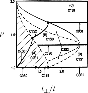
FIG. 12.: Phase diagram in the weak-coupling limit ($U\rightarrow 0$) given in ref. [53]; the numbers of the gapless charge and spin modes ($x$ and $y$, respectively) are denoted as C$x$S$y$ and $\rho\equiv 2-n$ ($n$ is the band filling). In the dark region all the three bands cross the Fermi level.

On the other hand, his result also indicates that two gapful spin modes exist in addition. While a spin gap certainly favors a singlet superconducting (SS) correlation when there is only one spin mode, we are in fact faced here with an intriguing problem of what happens when gapless and gapful spin modes coexist, since it may well be possible that the presence of gap(s) in some out of multiple spin modes may be sufficient for the dominance of a pairing correlation. Furthermore, as discussed below, the gaps of two spin modes emerge as an effect of the pair-tunneling process across the top and the bottom bands (Fig.4). This is reminiscent of the two-leg case and of the Suhl-Kondo mechanism. [34, 35] These have motivated us, in this section, to actually look at the correlation functions using the bosonization method[23] at the fixed point away from half-filling. Although in the three-leg case, we can consider the two boundary conditions across the legs, i.e., open boundary condition (OBC) and periodic boundary condition (PBC), here we concentrate on the open boundary condition (OBC) across the chains, where the central chain is inequivalent to the two edge chains. The reason is that we would like to (i) study the realistic boundary condition corresponds to cuprates, and (ii) to avoid the frustration introduced in the periodic three-legs.

We find that the interchain SS pairing across the central and edge chains is the dominant correlation, which is indeed realized due to the presence of the two gapful spin modes. On the other hand, the SDW correlation, which has a slowly-decaying power law for the intra-edge chain reflecting the gapless spin mode, coexists but is only subdominant. [43] Recently Schulz[45] has independently shown similar results for a subdominant $2k_{F}$ SDW and the interchain pairing correlations which are given in this section.

A Model and the Calculation

The three-leg Hubbard model with OBC is defined by the following Hamiltonian,

$$H= -t\sum_{\mu i\sigma}(c^{\dagger}_{\mu i\sigma}c_{\mu i+1\sigma}+{\rm h.c.})$$ (7)

$$-t_{\perp}\sum_{i\sigma}(c^{\dagger}_{\alpha i\sigma}c_{\beta i\sigma}+c^{\dagger}_{\beta i\sigma}c_{\gamma i\sigma}+{\rm h.c.})$$

$$+U\sum_{\mu i}n_{\mu i\uparrow}n_{\mu i\downarrow},$$

where $t(t_{\perp})$ is the intra-(inter-)chain hopping, $i$ labels the rung while $\mu=\alpha,\beta,\gamma$ labels the leg (with $\beta$ being the central one). In the momentum space we have

$$H= \sum_{k\sigma}\left(-2t{\rm cos}(k)-\sqrt{2}t_{\perp}\right)a^{\dagger}_{1k\sigma}a_{1k\sigma}$$ (11)

$$-2t\sum_{k\sigma}{\rm cos}(k)a^{\dagger}_{2k\sigma}a_{2k\sigma}$$

$$+\sum_{k\sigma}\left(-2t{\rm cos}(k)+\sqrt{2}t_{\perp}\right)a^{\dagger}_{3k\sigma}a_{3k\sigma}$$

$$+U\sum({\rm terms\ of\ the\ form}\ a^{\dagger}a^{\dagger}aa).$$

Here $a_{jk\sigma}$ annihilates an electron with lattice momentum $k$ in the $j$-th band ($j=1,2,3$), where $a_{jk\sigma}$ is related to $c_{\mu k\sigma}$ (the Fourier transform of $c_{\mu i\sigma}$) through a linear transformation,

$$\left(\begin{array}[]{c}c_{\alpha k\sigma}\\ c_{\beta k\sigma}\\ c_{\gamma k\sigma}\end{array}\right)=\left(\begin{array}[]{ccc}\frac{1}{2}&\frac{1}{\sqrt{2}}&\frac{1}{2}\\ \frac{1}{\sqrt{2}}&0&-\frac{1}{\sqrt{2}}\\ \frac{1}{2}&-\frac{1}{\sqrt{2}}&\frac{1}{2}\end{array}\right)\left(\begin{array}[]{c}a_{1k\sigma}\\ a_{2k\sigma}\\ a_{3k\sigma}\end{array}\right).$$ (21)

Hereafter we linearize the band structure around the fermi points as usual and neglect the difference in the fermi velocities of three bands, as is done for calculating the correlation functions directly in the weak-coupling theory for the two-leg case,[28, 31] which will be acceptable for the weak interchain hopping. These approximations enable us to calculate the correlation functions. The difference in fermi velocities of three bands will not be important qualitatively as long as we consider the case where three bands cross the fermi energy, for which Arrigoni’s result falls on the same strong coupling fixed point on the plane of interchain hopping and filling. In the following, we focus on the case in which all of three bands are away from half-filling.

The part of the Hamiltonian, $H_{\rm d}$, that can be diagonalized in the bosonization only includes forward-scattering processes in the band picture, and has the form

$$H_{\rm d} = H_{\rm spin}+H_{\rm charge},$$ (22)

$$H_{\rm spin} = \sum_{i}\frac{v_{\sigma i}}{4\pi}\int\ dx[\frac{1}{K_{\sigma i}}(\partial_{x}\phi_{i+})^{2}+K_{\sigma i}(\partial_{x}\phi_{i-})^{2}],$$ (23)

$$H_{\rm charge} = \sum_{i}\frac{v_{\rho i}}{4\pi}\int\ dx[\frac{1}{K_{\rho i}}(\partial_{x}\chi_{i+})^{2}+K_{\rho i}(\partial_{x}\chi_{i-})^{2}].$$ (24)

Here $\phi_{i+}$ is the spin phase field of the $i$-th band, $\chi_{i+}$ is the diagonal charge phase field, while $\phi_{i-}$($\chi_{i-}$) is the field dual to $\phi_{i+}$($\chi_{i+}$), $K_{\sigma i}$($K_{\rho i}$) the correlation exponent for the $\phi$($\chi_{i}$) phase with $v_{\sigma i}$($v_{\rho i}$) being their velocities. For the Hubbard-type interaction, we have $v_{\sigma i}=v_{F}$, $K_{\sigma i}$=1 for all $i$’s, while $v_{\rho 1}=v_{F}$, $v_{\rho 2}=v_{F}\sqrt{1-4g^{2}}$, $v_{\rho 3}=v_{F}\sqrt{1-g^{2}/4}$, $K_{\rho 1}=1$, $K_{\rho 2}=\sqrt{(1-2g)/(1+2g)}$, $K_{\rho 3}=\sqrt{(1-g/2)/(1+g/2)}$, where $g=U/2\pi v_{F}$ is the dimensionless coupling constant. The derivation of the above equation is given in the Appendix.

The diagonalized charge field $\chi_{i\pm}$ is linearly related to the initial charge field $\theta_{i\pm}$ of the $i$-th band as

$$\left(\begin{array}[]{c}\theta_{1\pm}\\ \theta_{2\pm}\\ \theta_{3\pm}\end{array}\right)=\left(\begin{array}[]{ccc}\frac{1}{\sqrt{2}}&\frac{1}{\sqrt{3}}&\frac{1}{\sqrt{6}}\\ 0&\frac{1}{\sqrt{3}}&-\sqrt{\frac{2}{3}}\\ -\frac{1}{\sqrt{2}}&\frac{1}{\sqrt{3}}&\frac{1}{\sqrt{6}}\end{array}\right)\left(\begin{array}[]{c}\chi_{1\pm}\\ \chi_{2\pm}\\ \chi_{3\pm}\end{array}\right),$$ (34)

where both $\theta_{i\pm}$ and $\phi_{\pm}$ are related to the field operator for electrons $\psi_{i+(-)\sigma}$, which annihilates an electron on the right-(left-) going branch in band $i$ as

$$\psi_{i+(-)\sigma}(x) = \frac{\eta_{i+(-)\sigma}}{2\pi\Lambda}{\rm exp}\{\pm ik_{iF}x$$ (36)

$$\pm\frac{i}{2}[\theta_{i+}(x)\pm\theta_{i-}(x)+\sigma(\phi_{i+}(x)\pm\phi_{i-}(x))]\}.$$

Here the $\eta_{ir\sigma}$’s are Haldane’s $U$ operators [50] which ensure the anti-commutation relations between electron operators through the relation, $\{\eta_{ir\sigma},\eta_{i^{\prime}r^{\prime}\sigma^{\prime}}\}_{+}=2\delta_{ii^{\prime}}\delta_{rr^{\prime}}\delta_{\sigma\sigma^{\prime}}$, $\eta_{ir\sigma}^{\dagger}=\eta_{ir\sigma}$.

There are still many scattering processes corresponding to both the backward and the pair-tunneling scattering processes, which cannot be treated exactly. Arrigoni examined the effect of such scattering processes by the perturbational renormalization-group technique. He found that the backward-scattering interaction within the first or the third band turn from positive to negative as the renormalization is performed and that the pair-tunneling processes across the first and third bands also become relevant. As far as the relevant scattering processes are concerned, the first (third) band plays the role of the bonding (anti-bonding) band in the two-leg case. At the fixed point the Hamiltonian density, $H^{*}$, then takes the form, in term of the phase variables,

$$H^{*} = -\frac{g_{b}(1)}{\pi^{2}\Lambda^{2}}{\rm cos}(2\phi_{1+}(x))-\frac{g_{b}(3)}{\pi^{2}\Lambda^{2}}{\rm cos}(2\phi_{3+}(x))$$ (38)

$$+\frac{2g_{ft}(1,3)}{\pi^{2}\Lambda^{2}}{\rm cos}(\sqrt{2}\chi_{1-}(x)){\rm sin}\phi_{1+}(x){\rm sin}\phi_{3+}(x),$$

where both $g_{b}(1)$ and $g_{b}(3)$ are negative large quantities, and $g_{ft}(1,3)$ is a positive large quantity.

This indicates that the phase fields $\phi_{1+}$, $\phi_{3+}$, and $\chi_{1-}$ are long-range ordered and fixed at $\pi/2$, $\pi/2$, and $\pi/\sqrt{2}$, respectively, which in turn implies that the correlation functions that contain $\phi_{1-}$, $\phi_{3-}$, and $\chi_{1+}$ fields decay exponentially. The renormalization procedure will affect the velocities and the critical exponents for the gapless fields, $\chi_{2\pm}$, $\chi_{3\pm}$, and $\phi_{2\pm}$, so that we should end up with renormalized $v^{*}$’s and $K^{*}$’s.

In principle, the numerical values of renormalized $v^{*}$’s and $K^{*}$’s for finite $g$ may be obtained from the renormalization equations as has been attempted for a double chain by Balents and Fisher [27], although it would be difficult in practice. However, at least in the weak-coupling limit, $g\rightarrow 0$, to which our treatment is meant to fall upon, we shall certainly have $v^{*}\simeq v_{F}$ and $K^{*}\simeq 1$ for gapless modes even after the renormalization procedure.

B Results for the Correlation Functions

Now we are in position to calculate the correlation functions, since the gapless fields have already been diagonalized, while the remaining gapful fields have the respective expectation values. The details of the calculation of the correlation functions are given in the Appendix. The two-particle correlation functions which include the following two particle operators in the band description are shown to have a power-law decay:

(1) operators constructed from two operators involving only the second band (since the charge and the spin phases are both gapless, electrons in this band should have the usual TL-liquid behavior),

(2) order parameters of singlet superconductivity within the first or third band, $\psi_{1+\uparrow(\downarrow)}\psi_{1-\downarrow(\uparrow)}$, $\psi_{3+\uparrow(\downarrow)}\psi_{3-\downarrow(\uparrow)}$.

As a result, the order parameters that possess power-law decays should be the following,

(A) The correlations within each of the two edge ($\alpha$ and $\gamma$) chains or across the two edge chains:

(a) $2k_{F}$ CDW,

$O_{{\rm intra}2k_{F}{\rm CDW}}=\psi_{\alpha(\gamma)+\uparrow}^{\dagger}\psi_{\alpha(\gamma)-\uparrow}$;

$O_{\rm interCDW}=\psi_{\alpha(\gamma)+\uparrow}^{\dagger}\psi_{\gamma(\alpha)-\uparrow},$

(b) $2k_{F}$ SDW,

$O_{\rm intraSDW}=\psi_{\alpha(\gamma)+\uparrow}^{\dagger}\psi_{\alpha(\gamma)-\downarrow}$;

$O_{\rm interSDW}=\psi_{\alpha(\gamma)+\uparrow}^{\dagger}\psi_{\gamma(\alpha)-\downarrow}$,

(c) singlet pairing (SS),

$O_{\rm intraSS}=\psi_{\alpha(\gamma)+\uparrow}\psi_{\alpha(\gamma)-\downarrow}$;

$O_{\rm interSS}=\psi_{\alpha(\gamma)+\uparrow}\psi_{\gamma(\alpha)-\downarrow}$,

(d) triplet pairing (TS),

$O_{\rm intraTS}=\psi_{\alpha(\gamma)+\uparrow}\psi_{\alpha(\gamma)-\uparrow}$;

$O_{\rm interTS}=\psi_{\alpha(\gamma)+\uparrow}\psi_{\gamma(\alpha)-\uparrow}$,

(B) The $4k_{F}$ CDW which is written with four electron operators,

$O_{4k_{F}{\rm CDW}}=\psi_{\nu+\uparrow}^{\dagger}\psi_{\nu+\downarrow}^{\dagger}\psi_{\nu-\uparrow}\psi_{\nu-\downarrow}\ \ \ (\nu=\alpha,\beta,\gamma)$,

(C) The singlet pairing across the central chain ($\beta$) and edge chains (Fig.13),

$O_{\rm CESS}=\sum_{\sigma}\sigma(\psi_{\alpha+\sigma}+\psi_{\gamma+\sigma})\psi_{\beta-,-\sigma}$.

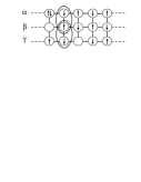
FIG. 13.: Schematic picture for the interchain (CESS) pairing in the doped three-leg Hubbard ladder.

In the band picture we can rewright $O_{\rm CESS}$ as comprising

$$O_{\rm CESS}\sim\sum_{\sigma}\sigma(\psi_{1+\sigma}\psi_{1-,-\sigma}-\psi_{3+\sigma}\psi_{3-,-\sigma}).$$ (39)

We cannot easily name the symmetry of the pairing, although we naively might call this pairing d-wave-like in a similar sense as in the two-leg case, in which a pair is called d-wave when the pairing, in addition to being off-site, consists of a bonding band and an anti-bonding band pairs with opposite signs.[27, 28, 30, 31, 33] Thus the edge-chain SDW correlation has a power-law decay, while the SDW correlation within the central chain decays exponentially since it consists of the terms containing $\phi_{1-}$ and/or $\phi_{3-}$ phases. Although we consider the case away from half-filling, the SDW correlation should obviously be more enhanced at half-filling. The experiments at half-filling do not contradict the present results, since the experiments should detect the total SDW correlation of all the chains and the SDW correlation is more enhanced at half-filling. However the present theory corresponds only to the infinitesimally small interaction in principle, although the actual cuprates have a strong interactions between electrons.

Intra- or inter-edge correlation functions have to involve forms bilinear in $a_{2k\sigma}$ in eq.(21). They are described in terms of the charge field $\theta_{2}$ for the second band, which does not contain $\chi_{1}$, a phase-fixed field (see eq.(34)). Thus the edge-channel correlations are completely determined by the character of the second band (the Luttinger-liquid band), while the other phase fields, being gapful, are irrelevant. The final result for the edge-channel correlations at large distances, up to $2k_{F}$ oscillations, is as follows regardless of whether the correlation is intra- or inter-edge:

$$\langle O_{2k_{F}{\rm CDW}}(x)O_{2k_{F}{\rm CDW}}^{\dagger}(0)\rangle \sim x^{-\frac{1}{3}(K_{\rho 2}^{*}+2K_{\rho 3}^{*})-1},$$ (40)

$$\langle O_{\rm SDW}(x)O_{\rm SDW}^{\dagger}(0)\rangle \sim x^{-\frac{1}{3}(K_{\rho 2}^{*}+2K_{\rho 3}^{*})-1},$$ (41)

$$\langle O_{\rm SS}(x)O_{\rm SS}^{\dagger}(0)\rangle \sim x^{-\frac{1}{3}(\frac{1}{K_{\rho 2}^{*}}+\frac{2}{K_{\rho 3}^{*}})-1},$$ (42)

$$\langle O_{\rm TS}(x)O_{\rm TS}^{\dagger}(0)\rangle \sim x^{-\frac{1}{3}(\frac{1}{K_{\rho 2}^{*}}+\frac{2}{K_{\rho 3}^{*}})-1}.$$ (43)

(where we have put $K_{\sigma}^{*}=1$ for the present spin-independent interaction.[45]) In addition, the $4k_{F}$ CDW correlation decays as

$$\langle O_{4k_{F}{\rm CDW}}(x)O_{4k_{F}{\rm CDW}}^{\dagger}(0)\rangle\sim x^{-\frac{2}{3}(2K_{\rho 2}^{*}+K_{\rho 3}^{*})}.$$ (44)

By contrast, if we look at the pairing $O_{\rm CESS}(x)$ across the central chain and the edge chains, this pairing, which circumvents the on-site repulsion and is linked by the resonating valence bonding across the neighboring chains, is expected to be stronger than other correlations as in the two-leg case. The correlation function for $O_{\rm CESS}(x)$ is indeed calculated to be

$$\langle O_{\rm CESS}(x)O_{\rm CESS}^{\dagger}(0)\rangle\sim x^{-\frac{1}{3}(\frac{1}{K_{\rho 2}^{*}}+\frac{1}{2K_{\rho 3}^{*}})}.$$ (45)

From the calculations given in the Appendix, we can see that the interchain pairing exploits the charge gap and the spin gaps to reduce the exponent of the correlation function, in contrast to the intra-leg pairing. In addition to that, we also find that the roles of the first (third) band corresponds to those of the bonding (anti-bonding) band in the two-leg case, as far as the dominant pairing correlation is concerned. If we consider the weak-interaction limit ($U\rightarrow+0$) as in the two-leg case, all the $K^{*}$’s will tend to unity, where the CESS correlation decays as $x^{-1/2}$ while those of other correlations decays as $x^{-2}$ at long distances. Thus, at least in this limit, the CESS correlation dominates over the others. The duality (which dictates that the pairing and density-wave exponents are reciprocal of each other[30]) is similar to that in the two-chain case, in which the interchain SS decays as $x^{-1/2}$ while that of the $4k_{F}$ CDW decays as $x^{-2}$.

In this section, we have studied correlation functions using the bosonization method at the renormalization-group fixed point, which was obtained by Arrigoni, away from half-filling in the region where the fermi level intersects all the three bands in the non-interacting case. We found that the interchain singlet pairing across the central chain and either of the edge chains is the dominant correlation contrary to the naive ‘even-odd’ conjecture for the superconductivity in ladder systems, while the SDW correlations in two edge chains coexist but are subdominant. The power law decay of the SDW correlation does not contradict with the even-odd conjecture at the half-filling, where the Umklapp scattering play a important role resulting in an enhancement of the SDW correlation.

The renormalization study is valid only for infinitesimally small interaction strengths and sufficiently small interchain hoppings in principle, while the actual cuprates have strong interactions between electrons, so that the relevance of the present results to the real materials is uncertain. However the present study suggests an important theoretical message that the dominance of superconductivity only requires the existence of gap(s) in some spin modes when there are multiple modes in multi-leg ladder systems no matter whether the number of legs is odd or even.

IV QMC study of the pairing correlation in the three-leg Hubbard ladder

In the previous section, we have discussed the correlation functions in the three-leg Hubbard ladder within the weak-coupling theory. A key point in the previous section is that the gapless and the gapful spin excitations coexist in a three-leg ladder and the modes give rise to a peculiar situation where a specific singlet pairing across the central and edge chains (CESS pairing), that may be roughly a d-wave pairing, is dominant, while the $2k_{F}$ SDW on the edge chains simultaneously shows a subdominant but still long-tailed (power-law) decay associated with the gapless spin mode. This result is stimulating since it serves as a counter-example of a naive ‘even-odd’ conjecture.

However, there is a serious question about these weak-coupling results as discussed in the two-leg case in Sec.II. First, only for infinitesimally small interactions and sufficiently small hoppings are the results in Sec.III guaranteed to be valid in principle. Furthermore, when there is a gap in the excitation, the renormalization flows into a strong-coupling regime, so that the weak-coupling theory might break down even for small $U$. Hence it is imperative to study the problem from an independent numerical method for an intermediate strength of the Hubbard $U\sim t$ and an interchain hopping $t_{\perp}\sim t$. Although such a comparison of the numerical result for $U\sim t$ with the weak-coupling theory has been done for the two-leg system in Sec.II, this does not necessarily shed light on the situation in the three-leg case, where gapless and gapful modes coexist. In this section, it is shown that the QMC result for the three-leg Hubbard ladder indeed turns out to exhibit an enhancement of the pairing correlation even for finite coupling constants, $U/t=1\sim 2$.[46]

In addition, we also study the effects of various Umklapp processes at special fillings as in the two-leg case keeping in mind the above Arrigoni’s work[44] which also studied the effects of some Umklapp processes with the weak-coupling theory.

Throughout this section, we concentrate on the case in which all three bands cross the Fermi surface to explore the properties of a three-band system.

The projector Monte Carlo method is employed [25, 26] to investigate the ground-state pairing correlation function $P(r)\equiv\langle O^{\dagger}_{j}O_{j+r}\rangle$, where $O_{i}\equiv O_{CESS}(i)=(c_{\alpha i\sigma}+c_{\gamma i\sigma})c_{\beta i-\sigma}-(c_{\alpha i-\sigma}+c_{\gamma i-\sigma})c_{\beta i\sigma}$. We assume the periodic boundary condition along the chain direction, $c_{N+1}\equiv c_{1}$, where $N$ is the number of rungs. We first consider the case where the intra- and the inter-band Umklapp processes are irrelevant because that is where the above-mentioned weak-coupling theory is valid. The details of the QMC calculation are similar to those for our QMC study for the two-leg case. Specifically, the negative-sign problem makes the QMC calculation feasible for $U\leq 2t$ as in the two-leg case. We set $t=1$ hereafter.

In the two-leg case with a finite $U$, we have found an interesting property for finite systems: the pairing correlation is enhanced in agreement with the weak-coupling theory only when the single-electron energy levels of the bonding and the anti-bonding bands lie close to each other around the Fermi level (which is certainly the case with an infinite system). When the levels are misaligned (for which a 5% change in $t_{\perp}$ is enough), the enhancement of the pairing correlation dramatically vanishes. In the weak-coupling theory, the ratio of the spin gap to the level offset is assumed to be infinitely large at the fixed point of the renormalization flow, so that the spin gap should naturally be detectable in finite systems only when the level offset is smaller than the gap.

We have found that this applies to the three-leg ladder as well, i.e., the pairing correlation is enhanced when the single-electron levels of the first and third bands lie close to each other. Hence we concentrate on such cases hereafter.

In the beginning we show in Fig.14 the result for $P(r)$ for $t_{\perp}=0.92$ with $U=1$ with the band filling $n=0.843=86$ electrons/(34 rungs$\times$ 3 sites). For this choice of $t_{\perp}$ the levels in the first and the third bands lie close to each other around the Fermi level within 0.01. We can see that a large enhancement over the $U=0$ result at large distances indeed exists. This is the key result of this section.

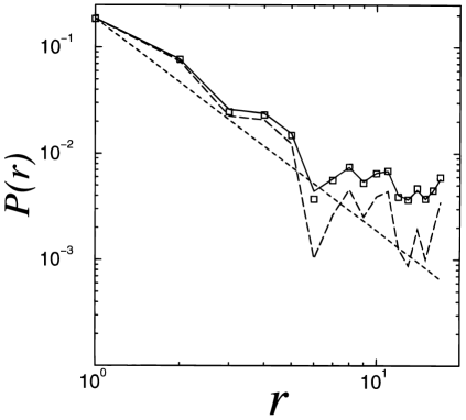
FIG. 14.: QMC result for the pairing correlation function, $P(r)(\Box)$, plotted against the real space distance $r$ in a three-leg Hubbard ladder with 34 rungs having 86 electrons for $U=1$ with $t_{\perp}=0.92$. The dashed line is the noninteracting result for the same system size, while the straight dashed line represents $\sim r^{-2}$. The solid line is a fit to a trial function (see text).

Although it is difficult to determine the decay exponent of $P(r)$, we can fit the data by supposing a trial function as expected from the weak-coupling theory as we did in the two-leg case,

$$P(r) = \frac{1}{\pi^{2}}\sum_{d=\pm}\{cr_{d}^{-1/2}$$ (47)

$$+[(2-c)-\cos(2k_{F1}r_{d})-\cos(2k_{F3}r_{d})]r_{d}^{-2}\}$$

Here $k_{F1}(k_{F3})$ is the non-interacting Fermi wave number of the first (third) band, while a constant $c$, which should vanish for $U=0$, is here least-square fit (by taking logarithm of the data) as $c=0.05$. As in the two-leg case, since we assume the periodic boundary condition, we have to consider contributions from both ways around, so there are two distances between the 0-th and the $r$-th rung, i.e., $r_{+}=r$ and $r_{-}=N-r$. The overall decay should be $1/r^{2}$ as in the single-chain case, while the term $c/r^{1/2}$, the dominant correlation at large distances, is borrowed from the weak-coupling result.[43, 45] The QMC result for a finite $U=1$ fits to the trial form (solid line in Fig.14) surprisingly accurately. A finite $U$ may give some corrections to these functional forms, but even when we best-fit the exponent itself as $c/r^{\alpha}$ in place of $c/r^{1/2}$, we obtain $\alpha<0.7$ with a similar accuracy.

In Fig.15, we show the result for a larger interaction $U=2$. The result again shows an enhanced pairing correlation at large distances. However, the enhancement is slightly reduced than that in the $U=1$ case. This is consistent with the weak-coupling theory, in which $K^{*}_{\rho}$’s should decrease with $U$.

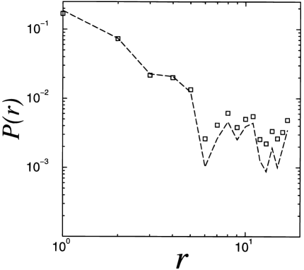
FIG. 15.: Plot similar to that in Fig.14 for $U=2$.

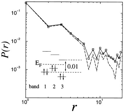
FIG. 16.: Similar plot as in Fig.14 for a 38 rungs system having 82 electrons for $U=1$ with $t_{\perp}=0.685$. The inset schematically depicts the positions of energy levels for the noninteracting case.

Furthermore, we study if the presence of the second band around $E_{F}$ can be detrimental to superconductivity. In Fig.16, we make the single-electron energy levels of all the three bands lie close to each other around the Fermi level. This is accomplished here for $t_{\perp}=0.685$ and the band filling $n=0.719=82$ electrons/(38 rungs $\times$ 3 sites). The highest occupied level of the second band then lies between that of the first band and the lowest unoccupied level of the third band (lying above the highest occupied level of the first band by as small as 0.01, inset of Fig.16).

The result in Fig.16 for $U=1$ shows that the pairing correlation is enhanced as well. Thus we may consider that the second band does not hinder the enhancement of the pairing correlation in other bands. This is also consistent with the weak-coupling theory, in which all of the scattering processes connected with the second band are irrelevant. The fit of the correlation function to the trial one is again excellent with $c=0.03$.

In the remaining of this section, we discuss the effects of the Umklapp processes at special fillings to clarify the doping dependence. In the three-leg Hubbard model, the Umklapp processes can play an important role at specific band fillings.

Arrigoni[44] also studied the effect of Umklapp processes within the weak-coupling theory, although he did not calculate the correlation functions directly (see Fig.12). He studied two cases that have the relevant Umklapp processes.

(i) the half-filled case.

(ii) the case when the bottom band is half-filled, in which the intraband Umklapp process may become relevant within the first band.

In both cases, the Umklapp processes become relevant. In the former case, the system has a gapless spin excitation suggesting a power-law decaying AF correlation, as discussed by Arrigoni, for $t_{\perp}\sim t$, a region of interest. The phase is called a ‘C1S1’ regime, since there is one gapless mode in charge or spin mode. Although the existence of a gapless charge mode suggests that the system is not an insulator, a full charge gap is expected to appear for sufficiently large $U$. Then, the pairing correlation will be suppressed, although the direct calculation has not been done. (As discussed in Sec.II, there are two kinds of charge gaps. The one, which is produced by the pair-tunneling processes, favors the pairing correlation as in the previous section, while the other, which is produced by the Umklapp processes, suppress the pairing correlation as in the present section.)

In the latter case, the Umklapp process also becomes relevant resulting in a ‘C2S3’ phase with the two gapless charge modes and three gapless spin modes and the singlet-pair of holes or electrons is prevented from binding. Thus the pairing correlation will be not enhanced because of the absence of gapful spin mode(s). This situation is reminiscent of the two-leg case, in which the spin gap is destroyed when the bonding band is half-filled. The Umklapp process within the first band in the present case is identified with that in the bonding band in the two-leg case, since the first (third) band corresponds to the bonding (anti-bonding) band as far as the pairing correlation is concerned as discussed in Sec.III.

Given this situation, our motivation here is to look at the pairing correlation and, in addition, to explore in which case the Umklapp scattering does or does not affect the pairing correlation. We study the above two cases and also study the case in which the second band is half-filled. Namely, we wish to see whether both the first and the third bands, which involve the pairing order parameter, are affected by an indirect effect of the Umklapp process in the second band. Such a situation emerges in ladder systems with three or larger number of legs.

We have tuned the value of $t_{\perp}$ to ensure that the level offset $(\Delta\varepsilon)$ between the first and the third bands at the Fermi level is as small as O($0.01$) for $U=0$ to single out the effect of Umklapp processes from those due to large values of $\Delta\varepsilon$. Ideally, we should make the single electron energy levels of all the three bands lie close to each other around the Fermi level but that is impossible within the tractable system sizes. However, when the Umklapp process is relevant within the first or the third band, the aligned levels of the bands should favor the pairing, so that if the pairing correlation is suppressed, we can infer that the suppression is not an artifact. On the other hand, when the level of the second band is misaligned from $E_{F}$, one may naively think that the effect of the Umklapp process within the band becomes obscured. However, the effect of the Umklapp processes should in fact be enhanced when the highest occupied level derivate from $E_{F}$, since the Umklapp processes become well-defined if the highest occupied level is doubly occupied.

In the beginning we look at the half-filling (Fig.17). Indeed, no enhancement of the pairing correlation is found and the over all decaying form is similar to the $U=0$ result as in the two-leg case at half-filling.

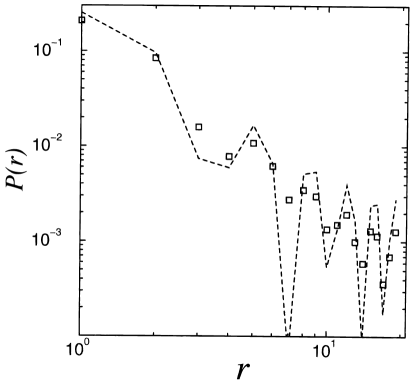
FIG. 17.: Pairing correlation $P(r)$ ($\Box$) against $r$ for a 38 rungs system for $U=2$ with $t_{\perp}=0.955$ and 114 electrons (half-filling). The dashed line represents the noninteracting result.

When $n$ is decreased to make the second band half-filled, the enhanced pairing correlation is found (Fig.18). Possibilities are either the Umklapp process is not relevant, or it is relevant but does not affect the other bands. In the latter case, a density-wave correlation might be dominant due to a charge gap opening by the Umklapp scattering. However, at least in the sense of the weak-coupling theory, the charge gap in the second band only enhances the density-wave correlation at long distances from $r^{-2}$ to $r^{-1}$ (unity, the value of the exponent, comes from the gapless spin mode and it should be independent to $U$) in the weak-coupling limit and thus the pairing correlation may still remain dominant for small $U$.

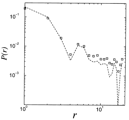
FIG. 18.: Pairing correlation $P(r)$ ($\Box$) against $r$ for a 38 rungs system for $U=2$ with $t_{\perp}=0.87$ and 110 electrons (the half-filled second band). The dashed line represents the noninteracting result.

Although we cannot decide which of the above two possibilities applies, we do have a unique situation where the pairing correlation is enhanced despite the Umklapp processes being possible. This interesting situation does not appear in the two-leg ladder.

Lastly, we study the case so that the first band is half-filled when $n$ is further decreased and $t_{\perp}$ is also decreased (Fig.19). In this case, we again observe no enhancement in $P(r)$, as expected from the weak-coupling theory and the above discussion.

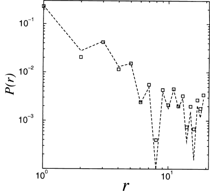
FIG. 19.: Pairing correlation $P(r)$ ($\Box$) against $r$ for a 38 rungs system for $U=2$ with $t_{\perp}=0.725$ and 74 electrons (the half-filled first band). The dashed line represents the noninteracting result.

In this section, we have shown with the projector quantum Monte Carlo method that the enhancement of the pairing correlation expected from the results in the previous section is indeed found even for the intermediate interaction strengths($U\sim 2t$) and the interchain hoppings($t_{\perp}\sim t$). The features of the enhancement is similar to that in the two-leg case.

We have also studied the cases where the Umklapp processes can be relevant. Especially, we found that the enhancement of the pairing correlation is not affected by the intraband Umklapp process within the second band which does not involve the pairing order parameter.

V Pairing correlation in finite systems — a case study for the 1D attractive Hubbard model

As we have seen in sections 2 (two-leg ladder) and 4 (three-leg ladder), QMC result for the pairing correlation in Hubbard ladders are consistent with the weak-coupling prediction when the highest occupied level and the lowest unoccupied level (called the level offset $\Delta\epsilon$ hereafter) in the relevant free-electron bands are made to lie close to each other. A similar situation is also found to occur in a QMC study of the single chain with distant transfers ($t-t^{\prime}-U$ model).[38]

We believe that small level offsets should be required to mimic the thermodynamic limit (bulk systems), where this quantity is infinitesimal. However, we have to quantify the criterion systematically. Otherwise, the results obtained in the previous section may be taken as an uncontrolled finite size effect. In this section we actually give a circumstantial evidence for justifying that we can indeed quantify this, with which we can tell that the results in the previous sections are meaningful.

We start with asking ourselves the following question. Let us take a model (such as the attractive Hubbard model with an attractive interaction $U<0$) that is known to superconduct. For a bulk system we know that the pairing correlation should have an slowly decaying asymptotic behavior for arbitrary $U\neq 0$, but in a numerical calculation such as QMC the tractable system size is limited, so that it is inconceivable that a slowly decaying asymptotic behavior is obtained even for, say, $|U|=0.01t$. So the question is what is the requirement for such an asymptotic behavior to be detectable in finite size systems.

We shall conclude in this section that the level offset as compared with the spin gap is the key ingredient. The criterion will also shed light on numerical calculations for systems which may possibly have small spin gaps.

As a case study, we take here the 1D attractive Hubbard model. This is because the model is exactly solvable with the Bethe Ansatz[49], so that we know the exact form of the correlation function as well as the value of the spin gap for arbitrary values of parameters. We compare this with QMC results for the pairing correlation for system sizes exceeding one hundred sites. We deliberately choose small attractions to look into the case where the spin gap is small.

Let us first briefly recapitulate the exact result for the 1D attractive Hubbard model, whose Hamiltonian is given by

$${\cal H}=-t\sum_{i\sigma}(c_{i\sigma}^{\dagger}c_{i+1\sigma}+{\rm h.c.})+U\sum_{i}n_{i\uparrow}n_{i\downarrow}\;\;\;\;(U<0)$$ (48)

in standard notations. We consider the case where the numbers of up-spin and down-spin electrons coincide. In this case, the spin gap is present for all the values of $U<0$ and the band filling $n$. At half filling $(n=1)$, the pairing correlation decays as $1/r$ with the real space distance $r$, regardless of the value of $U$. Note that the power is reduced abruptly by unity from the power (=2) for $U=0$ as soon as an infinitesimal $U$ is switched on. This is an effect of the spin gap, which opens as soon as an infinitesimal $U$ is switched on, this is due to the fact that the spin phase is locked to give a long range order for its contribution to the pairing correlation function for $U<0$. For a general value of $n$ the pairing correlation decays as $1/r^{1/K_{\rho}}$, where $(1\leq)K_{\rho}(<2)$, an exponent appearing in the Tomonaga-Luttinger theory, monotonically increases with $|U|$, and decreases with $n(\leq 1)$.

We have adopted the projector Monte Carlo method to calculate the on-site singlet pairing correlation function

$$P(r)=\langle c_{i\uparrow}^{\dagger}c_{i\downarrow}^{\dagger}c_{i+r\downarrow}c_{i+r\uparrow}\rangle$$ (49)

in the ground state. The calculation is free from the negative sign problem because we are considering the case of attractive $U$.[25] All the calculations are performed for a 114-site system. We consider the case where the closed shell condition (non-degenerate free-electron Fermi sea) is full-filled, so that there is a finite gap $\Delta\varepsilon$ between the highest occupied level and the lowest unoccupied level. To evaluate the decaying power of the pairing correlation, we least-square fit the numerical result to $1/r^{\alpha}$ in the range $r=6\sim 27$ by taking logarithm of the data. In this range the periodic boundary condition is seen to have little effect. Although a cosine-like fluctuation is obviously present in the data, fitting all of the points in a finite range should average this effect out, namely, fitting $\cos(kr)/r^{\beta}$ to a form $a/r^{\gamma}$ would give $a\sim 0$.

In Fig.20, we first present results for half filling $(n=1)$, where the pairing correlation has an asymptotic behavior like $\sim 1/r$ regardless of $U$. Our QMC result for $U=-t$ shows that the power is $\alpha\sim 1.4$ in contradiction with the exact result. Only when $U$ becomes as large as 2 do we recover $\alpha\sim 1$.

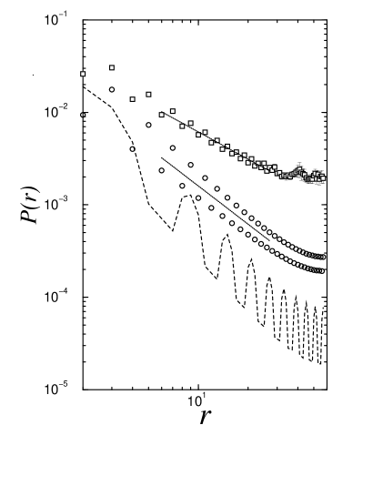
FIG. 20.: QMC result for the on-site pairing correlation function, $P(r)$, plotted against the real space distance $r$ in a 114-site 1D attractive Hubbard model at half filling. $U=0$ (dashed line), $U=-t$ ($\bigcirc$), $U=-2t$ ($\Box$). Straight dashed lines are least squares fit with $1/r^{\alpha}$ for $r=6\sim 27$.

Now, the spin gap $\Delta_{S}$ for this system size at $U=-t(-2t)$ estimated from the Bethe Ansatz is 0.12t (0.23t). If we take the ratio of these values to the level offset $\Delta\varepsilon$ around the Fermi level, which is $0.11t$, they give values 1.1 and 2.1, respectively. This suggests that the pairing correlation, which is governed by the spin gap, cannot be clearly detected unless $\Delta_{S}/\Delta\varepsilon$ is sufficiently large, in agreement with our speculation mentioned at the beginning of the present section. In fact $\Delta_{S}/\Delta\varepsilon$ is infinite in a bulk system, and we also assume an infinite $\Delta_{S}/\Delta\varepsilon$ in the Tomonaga-Luttinger theory as well.

In Fig.21, in order to confirm the point away from the half filling, we have also looked at $n=1/3$, where $\Delta\varepsilon(=0.055t)$ is smaller than that for $n=1$. The power for the pairing correlation is now $\alpha\sim 0.85$ for $U=-t$ form the Bethe Ansatz. The QMC result for $U=-t$ gives $\alpha\sim 0.9$, indicating that the numerical result is rather reliable already at $U=-t$ in this case. If we look at the level offset, $\Delta_{S}/\Delta\varepsilon\sim 1.6$ is indeed greater than that for $n=1$ and is closer to the case of $U=-2t$ for $n=1$. This result further confirms our view.

FIG. 21.: QMC result for $P(r)$ with $U=-t$. $n=1$ ($\bigcirc$), $n=1/3$ ($\Box$).

In conclusion, we have shown that the effect of the spin gap can be clearly seen in the correlation function of finite size systems only when the size of the gap is sufficiently large compared to the discreteness of the one-body energy levels. Combining the results for the Hubbard ladders and for the $t-t^{\prime}-U$ model, we believe that this is the case in general: A criterion for reproducing the correct form of the correlation functions is to make $\Delta_{S}/\Delta\varepsilon$ large. This implies that to reproduce the correct asymptotic behavior of the correlation functions in models having small spin gaps, very large systems are required. An alternative way is to tune, if possible, the values of the parameters so that $\Delta\varepsilon$ becomes small around the Fermi level, as we have done for ladders.

One final point is, since $\Delta\varepsilon$ is defined as the level offset at $U=0$, the quantity can become ill-defined for large interactions, where we have to consider that the quantity should be renormalized.

VI Summary

In the present paper, we have studied the pairing correlation in the Hubbard ladder with two(even) or three(odd) number of legs. This has been motivated from a conjecture due to Rice et al. that an even-numbered ladder should exhibit dominance of the interchain singlet pairing correlation as expected from the persistent spin gap away from half-filling. Naively, one can then expect that an odd-numbered ladder should not exhibit dominance of the pairing correlation reflecting the presence of gapless spin excitations.

We have first considered the two-leg Hubbard ladder model. In the weak-coupling theory, in which the interactions are treated with the perturbative renormalization-group method, a d-wave like pairing correlation becomes dominant reflecting a spin gap in the two-leg Hubbard ladder. The relevant scattering processes are the pair-tunneling process across the bonding and the anti-bonding bands and the backward-scattering process within each band. The pair-tunneling process is reminiscent of the Suhl-Kondo mechanism for superconductivity in the transition metals with a two-band structure. However, the weak-coupling theory is correct only for infinitesimally small interactions in principle. Thus the calculation for finite interaction $U$ is needed, but existing numerical calculations for finite $U$ have been controversial.

In Sec.II, we have applied the projector Monte Carlo method to investigate the pairing correlation function in the ground state for finite $U$. We conclude that the discreteness of energy levels in finite systems affects the pairing correlation enormously, where the enhanced pairing correlation is indeed detected for intermediate interaction strengths if we tune the parameters so as to align the discrete energy levels of bonding and anti-bonding bands at the Fermi level in order to mimic the thermodynamic limit. The enhancement of the pairing correlation in the $U=2t$ case is smaller than that in the $U=t$ case. This is consistent with the weak-coupling theory in which the pairing correlation decays as $r^{-1/(2K_{\rho})}$ ($K_{\rho}$ is the critical exponent of the gapless charge mode) at long distances and $K_{\rho}$ is a decreasing function of $U$.

In the cases where interband or intraband Umklapp process is possible, the pairing correlation is not enhanced. This result is also consistent with the weak-coupling theory.

We then moved onto the correlation functions in the three-leg Hubbard ladder model in Sec.III. Whether the above ‘even-odd’ conjecture holds for the simplest-odd ladder (i.e. the three-leg ladder) with a plural number of charge and spin modes is an important problem. This has remained an open question, since there had been no results for the pairing correlation function in the three-leg $t-J$ or Hubbard ladder models.

A key is the coexistence of gapless and gapful spin excitations in the doped three-leg Hubbard ladder. This has been analytically shown from the correlation functions starting from the phase diagram obtained by Arrigoni[44], who enumerated the numbers of the gapless charge and spin modes with the perturbative renormalization-group technique in the weak-coupling limit. If we turn to the correlation functions, we have found that the coexisting gapful and gapless modes give rise to a peculiar situation where a specific pairing across the central and edge chains (roughly a d-wave pairing) is dominant, while the $2k_{F}$ SDW on the edge chains simultaneously shows a subdominant but still long-tailed (power-law) decay associated with the gapless spin mode. The relevant scattering processes are the pair-tunneling process between the top and the bottom bands and the backward-scattering process within the top and the bottom bands. The situation is rather similar to the two leg case where the pair-tunneling processes play an important role for the enhanced pairing correlation. Schulz[45] has independently obtained results for both the SDW and the pairing correlations which are similar to those given in Sec.III.

However, as discussed in the two-leg case, it is not clear whether the weak-coupling results might be applicable only to infinitesimally small interaction strengths. In Sec.IV, we have thus checked the pairing correlation in the three-leg Hubbard ladder with the QMC method tuning the parameters so as to align the discrete energy levels of the first and third bands at the Fermi level as in the two-leg case. The enhanced pairing correlation is indeed detected even for intermediate interaction strengths in the three-leg ladder. The enhancement of the pairing correlation in the $U=2t$ case is smaller than that in the $U=t$ case as in the two-leg case in Sec.II. This result is consistent with the weak-coupling theory in Sec.III in a similar reason with that in the two-leg case. Namely, the exponent of the pairing correlation is a decreasing function of $K_{\rho}$’s which should decrease with $U$.

Various effects of the Umklapp processes have also been discussed. Especially, it is found that the enhancement of the pairing correlation is not affected by the intraband Umklapp process within the second band which does not involve the pairing order parameter. The key message obtained in the present paper, is that the dominance of the pairing correlation only requires the existence of gap(s) in not all but some of the spin modes. This is independent to whether the number of legs is even(two) or odd(three).

There are still important open questions. One is how the Hubbard model can possibly be related to real systems such as the cuprates. Specifically, One should study the two-leg and/or three-leg Hubbard ladder for larger $U$, where the dominance of the pairing correlation might be lost. Furthermore, the three-leg $t-J$ model should be studied to be compared with the Hubbard ladder. It would also be interesting to further investigate ladder systems with larger numbers of legs. The Hubbard ladders with more large number of legs is also of interest, since it may have a key point to understand the two-dimensional systems. More recently, Lin et al.[51] have examined the weak-coupling phase diagram for the four-leg Hubbard ladder where the pairing correlation is the most dominant in wide parameter region.

Finally, in Sec.V, a QMC study for the pairing correlation in the 1D attractive Hubbard model is given. The model can be exactly solved by Bethe Ansatz, so that we know the exact form of the correlation functions at long distances and the values of the spin gaps. A QMC study has shown that the effect of the spin gap can be clearly seen in the pairing correlation function of finite size systems and the behavior at long distances is consistent with the exact result only when the size of the gap is sufficiently large compared to the discreteness of the one-body energy levels. The result is a circumstantial evidence to justify the enhancement of the pairing correlation in Sec.II and Sec.IV and combining this result, we believe that this is the case in general for finite size systems.

We are grateful to Professor H.J. Schulz for directing our attention to refs.[3] and [45]. We wish to thank E. Arrigoni for sending us his work prior to publication. We also acknowledge helpful discussions with Professors M. Ogata, Y. Takada, H. Fukuyama, M. Imada, A. Fujimori, N. Môri, M. Azuma, Z. Hiroi, and J. Akimitsu. Numerical calculations were performed on a FACOM VPP 500/40 at the Supercomputer Center, Institute for Solid State Physics, the University of Tokyo and on a HITAC S3800/280 at the Computer Center of the University of Tokyo. For the latter facility we thank Professor Y. Kanada for support in a Project for Vectorized Super Computing. This work was also supported in part by a Grant-in-Aid for Scientific Research from the Ministry of Education, Science, Sports, and Culture of Japan. One of the authors (T.K.) acknowledges the Japan Society for the Promotion of Science for a fellowship.

A Calculation Method in Sec.III

1 Derivation of eq.(3.4)

Here we derive eq.(3.4) in the standard bosonization method. The intra- and the inter-band forward-scattering terms, which can be diagonally treated in the phase Hamiltonian as we will see in the following, are produced from the intrachain forward-scattering terms using eq.(3.3) as follows:

$$\frac{2\pi v_{F}g}{L}\sum_{k_{1},k_{2},q}\sum_{\mu,\sigma,\sigma^{\prime}}c_{\mu,+,k_{1},\sigma}^{\dagger}c_{\mu,-,k_{2},\sigma^{\prime}}^{\dagger}c_{\mu,-,k_{2}+q,\sigma^{\prime}}c_{\mu,+,k_{1}-q,\sigma}$$ (A12)

$$\equiv H_{{\rm f}}+\mbox{pair-tunneling terms},$$

$$=\frac{\pi v_{F}g}{4}\sum_{k_{1},k_{2},q}\sum_{\sigma,\sigma^{\prime}}[3a_{1,+,k_{1},\sigma}^{\dagger}a_{1,-,k_{2},\sigma^{\prime}}^{\dagger}a_{1,-,k_{2}+q,\sigma^{\prime}}a_{1,+,k_{1}-q,\sigma}$$

$$+4a_{2,+,k_{1},\sigma}^{\dagger}a_{2,-,k_{2},\sigma^{\prime}}^{\dagger}a_{2,-,k_{2}+q,\sigma^{\prime}}a_{2,+,k_{1}-q,\sigma}$$

$$+3a_{3,+,k_{1},\sigma}^{\dagger}a_{3,-,k_{2},\sigma^{\prime}}^{\dagger}a_{3,-,k_{2}+q,\sigma^{\prime}}a_{3,+,k_{1}-q,\sigma}$$

$$+2(a_{1,+,k_{1},\sigma}^{\dagger}a_{2,-,k_{2},\sigma^{\prime}}^{\dagger}a_{2,-,k_{2}+q,\sigma^{\prime}}a_{1,+,k_{1}-q,\sigma}$$

$$+a_{3,+,k_{1},\sigma}^{\dagger}a_{2,-,k_{2},\sigma^{\prime}}^{\dagger}a_{2,-,k_{2}+q,\sigma^{\prime}}a_{3,+,k_{1}-q,\sigma}$$

$$+a_{2,+,k_{1},\sigma}^{\dagger}a_{1,-,k_{2},\sigma^{\prime}}^{\dagger}a_{1,-,k_{2}+q,\sigma^{\prime}}a_{2,+,k_{1}-q,\sigma}$$

$$+a_{2,+,k_{1},\sigma}^{\dagger}a_{3,-,k_{2},\sigma^{\prime}}^{\dagger}a_{3,-,k_{2}+q,\sigma^{\prime}}a_{2,+,k_{1}-q,\sigma})$$

$$+3(a_{1,+,k_{1},\sigma}^{\dagger}a_{3,-,k_{2},\sigma^{\prime}}^{\dagger}a_{3,-,k_{2}+q,\sigma^{\prime}}a_{1,+,k_{1}-q,\sigma}$$

$$+a_{3,+,k_{1},\sigma}^{\dagger}a_{1,-,k_{2},\sigma^{\prime}}^{\dagger}a_{1,-,k_{2}+q,\sigma^{\prime}}a_{3,+,k_{1}-q,\sigma})]$$

$$+\mbox{pair-tunneling terms}.$$

Here $H_{\rm f}$ consists of the forward-scattering processes in the band description and the electron operator with index $+(-)$ belongs to the right-(left-) going branch. We prepare the following bosonic operators as in the usual single-chain case.

$$\alpha_{i,k}=\left\{\begin{array}[]{rl}&\Big{(}\frac{\pi}{kL}\Big{)}^{1/2}\sum_{i,p,\sigma}a_{i,+,p-k,\sigma}^{\dagger}a_{i,+,p,\sigma}\hskip 9.3894pt\quad\mbox{for $k>0$},\\ &\Big{(}\frac{\pi}{|k|L}\Big{)}^{1/2}\sum_{i,p,\sigma}a_{i,-,p+|k|,\sigma}^{\dagger}a_{i,-,p,\sigma}\quad\mbox{for $k<0$},\end{array}\right.$$ (A13)

$$\beta_{i,k}=\left\{\begin{array}[]{rl}&\Big{(}\frac{\pi}{kL}\Big{)}^{1/2}\sum_{i,p,\sigma}\sigma a_{i,+,p-k,\sigma}^{\dagger}a_{i,+,p,\sigma}\hskip 9.3894pt\quad\mbox{for $k>0$},\\ &\Big{(}\frac{\pi}{|k|L}\Big{)}^{1/2}\sum_{i,p,\sigma}\sigma a_{i,-,p+|k|,\sigma}^{\dagger}a_{i,-,p,\sigma}\quad\mbox{for $k<0$}.\end{array}\right.$$ (A14)

$\alpha_{i,k}(\beta_{i,k})$ corresponds to the charge(spin)-density excitation in band $i$. Note that, $\alpha_{i,k}$ and $\beta_{i,k}$ obey the boson commutation relation:

$$[\alpha_{i,k},\alpha_{i^{\prime},k^{\prime}}]=[\beta_{i,k},\beta_{i^{\prime},k^{\prime}}]=[\alpha_{i,k},\beta_{i^{\prime},k^{\prime}}]=[\alpha_{i,k},\beta_{i^{\prime},k^{\prime}}^{\dagger}]=0,$$ (A15)

$$[\alpha_{i,k},\alpha_{i^{\prime},k^{\prime}}^{\dagger}]=[\beta_{i,k},\beta_{i^{\prime},k^{\prime}}^{\dagger}]=\delta_{i,i^{\prime}}\delta_{k,k^{\prime}}.$$ (A16)

$H_{{\rm f}}$ is expressed in terms of only $\alpha_{i,k}$ as

$$H_{{\rm f}} = \frac{v_{F}g}{4}\sum_{k>0}k[3(\alpha_{1,k}^{\dagger}\alpha_{1,-k}^{\dagger}+\alpha_{3,k}^{\dagger}\alpha_{3,-k}^{\dagger}$$ (A17)

$$+ \alpha_{1,k}\alpha_{1,-k}+\alpha_{3,k}\alpha_{3,-k})+4(\alpha_{2,k}^{\dagger}\alpha_{2,-k}^{\dagger}+\alpha_{2,k}\alpha_{2,-k})$$ (A18)

$$+ 2(\alpha_{1,k}^{\dagger}\alpha_{2,-k}^{\dagger}+\alpha_{1,k}\alpha_{2,-k}+\alpha_{3,k}^{\dagger}\alpha_{2,-k}^{\dagger}+\alpha_{3,k}\alpha_{2,-k}$$ (A19)

$$+ \alpha_{1,-k}^{\dagger}\alpha_{2,k}^{\dagger}+\alpha_{1,-k}\alpha_{2,k}+\alpha_{3,-k}^{\dagger}\alpha_{2,k}^{\dagger}+\alpha_{3,-k}\alpha_{2,k})$$ (A20)

$$+ 3(\alpha_{1,k}^{\dagger}\alpha_{3,-k}^{\dagger}+\alpha_{1,k}\alpha_{3,-k}+\alpha_{3,k}^{\dagger}\alpha_{1,-k}^{\dagger}+\alpha_{3,k}\alpha_{1,-k})].$$ (A21)

(A22)

Furthermore we can rewrite the non-interacting part of the Hamiltonian $H_{0}$ as

$$H_{0}=v_{F}\sum_{i,p}|p|\alpha_{i,p}^{\dagger}\alpha_{i,p}+v_{F}\sum_{i,p}|p|\beta_{i,p}^{\dagger}\beta_{i,p}.$$ (A23)

Now we introduce the phase variables as in the single chain case by the following equations:

$$\theta_{i\pm} = i\sum_{k>0}\sqrt{\frac{\pi}{Lk}}e^{-\Lambda k/2}$$ (A25)

$$\times[e^{-ikx}(\alpha_{i,k}^{\dagger}\pm\alpha_{i,-k})-e^{ikx}(\alpha_{i,k}\pm\alpha_{i,-k}^{\dagger})],$$

$$\phi_{i\pm} = i\sum_{k>0}\sqrt{\frac{\pi}{Lk}}e^{-\Lambda k/2}$$ (A27)

$$\times[e^{-ikx}(\beta_{i,k}^{\dagger}\pm\beta_{i,-k})-e^{ikx}(\beta_{i,k}\pm\beta_{i,-k}^{\dagger})].$$

Here the phase variable $\phi_{i+}(\theta_{i+})$ can be regarded as the phase of the spin(charge)-density wave, while $\phi_{i-}(\theta_{i-})$ is the field dual to $\phi_{i+}(\theta_{i+})$.

From (B.7) and (B.8), we can write the diagonal part of the Hamiltonian, $H_{\rm d}=H_{0}+H_{\rm f}$, in terms of the phase variables as

$$H$$ _d= H_spin+H_charge, (A28)

$$H_{\rm spin}= \sum_{i}\frac{v_{F}}{4\pi}\int\ dx[(\partial_{x}\phi_{i+})^{2}+(\partial_{x}\phi_{i-})^{2}],$$ (A29)

$$H_{\rm charge}$$ (A30)

$$=\frac{v_{F}}{4\pi}\int\ dx \Big{[}\Big{(}1+\frac{3}{4}g\Big{)}(\partial_{x}\theta_{1+})^{2}+\Big{(}1-\frac{3}{4}g\Big{)}(\partial_{x}\theta_{1-})^{2}\Big{]}$$ (A31)

$$+\frac{v_{F}}{4\pi}\int\ dx \Big{[}\Big{(}1+g\Big{)}(\partial_{x}\theta_{2+})^{2}+\Big{(}1-g\Big{)}(\partial_{x}\theta_{2-})^{2}\Big{]}$$ (A32)

$$+\frac{v_{F}}{4\pi}\int\ dx \Big{[}\Big{(}1+\frac{3}{4}g\Big{)}(\partial_{x}\theta_{3+})^{2}$$ (A34)

$$+\Big{(}1-\frac{3}{4}g\Big{)}(\partial_{x}\theta_{3-})^{2}\Big{]}$$

$$+\frac{v_{F}g}{4\pi}\int\ dx \Big{[}(\partial_{x}\theta_{1+})(\partial_{x}\theta_{2+})-(\partial_{x}\theta_{1-})(\partial_{x}\theta_{2-})$$ (A36)

$$+(\partial_{x}\theta_{3+})(\partial_{x}\theta_{2+})-(\partial_{x}\theta_{3-})(\partial_{x}\theta_{2-})\Big{]}$$

$$+\frac{3v_{F}g}{8\pi}\int\ dx \Big{[}(\partial_{x}\theta_{1+})(\partial_{x}\theta_{3+})-(\partial_{x}\theta_{1-})(\partial_{x}\theta_{3-})\Big{]}.$$ (A37)

Thus $H_{\rm d}$ is separated to both the spin-part $H_{\rm spin}$ and the charge-part $H_{\rm charge}$. $H_{\rm charge}$ is also diagonalized by using eq.(3.5), while $H_{\rm spin}$ is already diagonalized. As a result, eq.(3.4) is easily obtained.

2 Calculation of Correlation Functions

Here we explain the method to derive the correlation functions. As examples, we here calculate the correlation functions of the intrachain singlet pairing in the edge chains and of the singlet pairing across the central and the edge chains. As stated in the text, the relevant scattering processes, are the pair-tunneling process between the first and the third bands and the backward-scattering process within the first or the third band.

The pair-tunneling process is expressed in terms of the phase variables as follows:

$$\psi_{3+\uparrow}^{\dagger}\psi_{3-\downarrow}^{\dagger}\psi_{1-\downarrow}\psi_{1+\uparrow}+\psi_{3+\downarrow}^{\dagger}\psi_{3-\uparrow}^{\dagger}\psi_{1-\uparrow}\psi_{1+\downarrow}$$ (A38)

$$+ \psi_{3+\downarrow}^{\dagger}\psi_{3-\uparrow}^{\dagger}\psi_{1+\uparrow}\psi_{1-\downarrow}+\psi_{3+\uparrow}^{\dagger}\psi_{3-\downarrow}^{\dagger}\psi_{1+\downarrow}\psi_{1-\uparrow}+{\rm h.c.}$$ (A39)

$$\propto \eta_{3+\uparrow}\eta_{3-\downarrow}\eta_{1-\downarrow}\eta_{1+\uparrow}{\rm exp}[i(\theta_{1-}-\theta_{3-}+\phi_{1+}-\phi_{3+})]$$ (A40)

$$+ \eta_{3+\downarrow}\eta_{3-\uparrow}\eta_{1-\uparrow}\eta_{1+\downarrow}{\rm exp}[i(\theta_{1-}-\theta_{3-}-\phi_{1+}+\phi_{3+})]$$ (A41)

$$+ \eta_{3+\downarrow}\eta_{3-\uparrow}\eta_{1+\uparrow}\eta_{1-\downarrow}{\rm exp}[i(\theta_{1-}-\theta_{3-}+\phi_{1+}+\phi_{3+})]$$ (A42)

$$+ \eta_{3+\uparrow}\eta_{3-\downarrow}\eta_{1+\downarrow}\eta_{1-\uparrow}{\rm exp}[i(\theta_{1-}-\theta_{3-}-\phi_{1+}-\phi_{3+})]+{\rm h.c.},$$ (A43)

$$= 2{\rm exp}[i(\theta_{1-}-\theta_{3-})][{\rm cos}(\phi_{1+}-\phi_{3+})-{\rm cos}(\phi_{1+}+\phi_{3+})]+{\rm h.c.},$$ (A44)

$$= 8{\rm cos}(\sqrt{2}\chi_{1-}){\rm sin}(\phi_{1+}){\rm sin}(\phi_{3+}).$$ (A45)

Here we have defined the product of the $U$ operators[50] as $\eta_{i+\uparrow}\eta_{i-\downarrow}=\eta_{i+\downarrow}\eta_{i-\uparrow}$, but this convention does not affect the correlation functions as in the two-leg case[28, 31].

The backward-scattering process within band $i$ is also expressed in terms of the phase variables through eq.(3.6) as

$$\psi_{i+\uparrow}^{\dagger}\psi_{i-\downarrow}^{\dagger}\psi_{i+\downarrow}\psi_{i-\uparrow}+{\rm h.c.}$$ (A46)

$$= \eta_{i+\uparrow}\eta_{i-\downarrow}\eta_{i+\downarrow}\eta_{i-\uparrow}{\rm exp}[-2i\phi_{i+}]+{\rm h.c.},$$ (A47)

$$= -2{\rm cos}(2\phi_{i+}).$$ (A48)

This and eq.(A41) give the eq.(3.7) in the text. In the beginning we calculate the correlation function of the intrachain pairing in an edge chain ($\alpha$ chain). The order parameter is expressed in the band description as

$$O_{\rm intraSS} \equiv \psi_{\alpha+\uparrow}\psi_{\alpha-\downarrow}$$ (A49)

$$\sim \frac{1}{4}[\psi_{1+\uparrow}\psi_{1-\downarrow}+\psi_{3+\uparrow}\psi_{3-\downarrow}+2\psi_{2+\uparrow}\psi_{2-\downarrow}],$$ (A50)

where we have picked up only the two-particle operators whose correlations show power-law decay at long distances. The correlations of the other two-particle operators correlation decay exponentially due to the gapful field(s). We can rewrite the above equation in the phase variables as

$$\psi_{1+\uparrow}\psi_{1-\downarrow}+2\psi_{2+\uparrow}\psi_{2-\downarrow}+\psi_{3+\uparrow}\psi_{3-\downarrow}$$ (A51)

$$\propto \eta_{1+\uparrow}\eta_{1-\downarrow}{\rm exp}[i(\theta_{1-}+\phi_{1+})]+\eta_{3+\uparrow}\eta_{3-\downarrow}{\rm exp}[i(\theta_{3-}+\phi_{3+})]$$ (A52)

$$+ 2\eta_{2+\uparrow}\eta_{2-\downarrow}{\rm exp}[i(\theta_{2-}+\phi_{2+})],$$ (A53)

$$= i{\rm exp}\Big{\{}i[(\frac{1}{\sqrt{2}}\chi_{1-}+\frac{1}{\sqrt{3}}\chi_{2-}+\frac{1}{\sqrt{6}}\chi_{3-})+\phi_{1+}]\Big{\}}$$ (A56)

$$+i{\rm exp}\Big{\{}i[(-\frac{1}{\sqrt{2}}\chi_{1-}+\frac{1}{\sqrt{3}}\chi_{2-}+\frac{1}{\sqrt{6}}\chi_{3-})+\phi_{3+}]\Big{\}}$$

$$+2i{\rm exp}[i(\theta_{2-}+\phi_{2+})],$$

$$= i{\rm exp}\Big{\{}i[(\frac{\pi}{2}+\frac{1}{\sqrt{3}}\chi_{2-}+\frac{1}{\sqrt{6}}\chi_{3-})+\frac{\pi}{2}]\Big{\}}$$ (A59)

$$+i{\rm exp}\Big{\{}i[(-\frac{\pi}{2}+\frac{1}{\sqrt{3}}\chi_{2-}+\frac{1}{\sqrt{6}}\chi_{3-})+\frac{\pi}{2}]\Big{\}}$$

$$+2i{\rm exp}[i(\theta_{2-}-\phi_{2+})],$$

$$= 2i{\rm exp}[i(\theta_{2-}-\phi_{2+})].$$ (A60)

Here we have fixed $\phi_{1+}=\phi_{3+}=\pi/2$ and $\chi_{1-}=\pi/\sqrt{2}$ as discussed in the text and the terms containing t he gapful fields are canceled out. Now we can calculate the correlation function:

$$\langle O_{{\rm intraSS}}(x)O_{{\rm intraSS}}(0)\rangle$$ (A61)

$$\propto \langle{\rm exp}[i(\theta_{2-}(x)-\phi_{2+}(x))]{\rm exp}[i(\theta_{2-}(0)-\phi_{2+}(0))]\rangle,$$ (A62)

$$= {\rm exp}[-\frac{1}{2}\{\langle(\theta_{2-}(x)-\theta_{2-}(0))^{2}\rangle+\langle(\phi_{2+}(x)-\phi_{2+}(0))^{2}\rangle\}],$$ (A63)

$$= {\rm exp}[-\frac{2\pi}{3L}(\frac{1}{K_{\rho 2}^{*}}+\frac{2}{K_{\rho 3}^{*}}+3)\sum_{k>0}\frac{e^{-\Lambda k}}{k}(1-{\rm cos}kx)],$$ (A64)

$$= {\rm exp}[-\frac{1}{6}(\frac{1}{K_{\rho 2}^{*}}+\frac{2}{K_{\rho 3}^{*}}+3){\rm log}(1+\frac{x^{2}}{\Lambda^{2}})],$$ (A65)

$$\sim x^{-\frac{1}{3}(\frac{1}{K_{\rho 2}^{*}}+\frac{2}{K_{\rho 3}^{*}})-1}.$$ (A66)

Now we calculate the correlation function of the singlet pairing across the central and the edge chains. The order parameter is expressed as

$$O_{\rm CESS} = (\psi_{\alpha+\uparrow}+\psi_{\gamma+\uparrow})\psi_{\beta-\downarrow}-(\psi_{\alpha+\downarrow}+\psi_{\gamma+\downarrow})\psi_{\beta-\uparrow},$$ (A67)

$$\sim \psi_{1+\uparrow}\psi_{1-\downarrow}-\psi_{3+\uparrow}\psi_{3-\downarrow}$$ (A69)

$$-(\psi_{1+\downarrow}\psi_{1-\uparrow}-\psi_{3+\downarrow}\psi_{3-\uparrow}).$$

Here again we pick up only the two-particle operators whose correlations show power-law decay. In terms of the phase variables, the order parameter can be rewritten as

$$\psi_{1+\uparrow}\psi_{1-\downarrow}-\psi_{3+\uparrow}\psi_{3-\downarrow}-\psi_{1+\downarrow}\psi_{1-\uparrow}+\psi_{3+\downarrow}\psi_{3-\uparrow}$$ (A70)

$$\propto \eta_{1+\uparrow}\eta_{1-\downarrow}{\rm exp}[i(\theta_{1-}+\phi_{1+})]-\eta_{3+\uparrow}\eta_{3-\downarrow}{\rm exp}[i(\theta_{3-}+\phi_{3+})]$$ (A71)

$$- \eta_{1+\downarrow}\eta_{1-\uparrow}{\rm exp}[i(\theta_{1-}-\phi_{1+})]+\eta_{3+\downarrow}\eta_{3-\uparrow}{\rm exp}[i(\theta_{3-}-\phi_{3+})],$$ (A72)

$$= i[{\rm exp}[i\{(\frac{1}{\sqrt{2}}\frac{\pi}{\sqrt{2}}+\frac{1}{\sqrt{3}}\chi_{2-}+\frac{1}{\sqrt{6}}\chi_{3-})+\frac{\pi}{2}\}]$$ (A76)

$$-{\rm exp}[i\{(-\frac{1}{\sqrt{2}}\frac{\pi}{\sqrt{2}}+\frac{1}{\sqrt{3}}\chi_{2-}+\frac{1}{\sqrt{6}}\chi_{3-})+\frac{\pi}{2}\}]$$

$$-{\rm exp}[i\{(\frac{1}{\sqrt{2}}\frac{\pi}{\sqrt{2}}+\frac{1}{\sqrt{3}}\chi_{2-}\frac{1}{\sqrt{6}}\chi_{3-})-\frac{\pi}{2}\}]$$

$$+{\rm exp}[i\{(-\frac{1}{\sqrt{2}}\frac{\pi}{\sqrt{2}}+\frac{1}{\sqrt{3}}\chi_{2-}+\frac{1}{\sqrt{6}}\chi_{3-})-\frac{\pi}{2}\}],$$

$$= -4i{\rm exp}[i(\frac{1}{\sqrt{3}}\chi_{2-}+\frac{1}{\sqrt{6}}\chi_{3-})].$$ (A77)

Calculation of the interchain pairing correlation function is quite similar to that of the intrachain pairing correlation.

$$\langle O_{\rm CESS}(x)O_{\rm CESS}(0)\rangle$$ (A78)

$$\propto \langle{\rm exp}[i(\frac{1}{\sqrt{3}}\chi_{2-}(x)+\frac{1}{\sqrt{6}}\chi_{3-}(x))]$$ (A80)

$$\times{\rm exp}[i(\frac{1}{\sqrt{3}}\chi_{2-}(0)+\frac{1}{\sqrt{6}}\chi_{3-}(0))]\rangle,$$

$$= {\rm exp}[-\frac{1}{2}\{\frac{1}{3}\langle(\chi_{2-}(x)-\chi_{2-}(0))^{2}\rangle$$ (A82)

$$+\frac{1}{6}\langle(\chi_{3-}(x)-\chi_{3-}(0))^{2}\rangle\}],$$

$$\sim x^{-\frac{1}{3}(\frac{1}{K_{\rho 2}^{*}}+\frac{1}{2K_{\rho 3}^{*}})}.$$ (A83)

From above calculations, we can see that the interchain pairing exploits the charge gap and the spin gaps to reduce the exponent of the correlation function, in contrast to the intrachain pairing.

REFERENCES

- [1] *Present address: Department of Physical Electrics, Hiroshima University, Higashi-hiroshima 739, Japan.
- [2] See for a review, E. Dagotto and T.M. Rice, Science 271 618 (1996) and references therein.
- [3] H.J. Schulz, Phys. Rev. B 34, 6372 (1986).
- [4] F.D.M. Haldane, Phys. Lett. A 93, 464 (1993).
- [5] Y. Nishiyama, N. Hatano, and M. Suzuki, J. Phys. Soc. Jpn 64, 1967 (1994).
- [6] T.M. Rice, S. Gopalan, and M. Sigrist, Europhys. Lett. 23 445 (1993); Physica B 199 & 200, 378 (1992).
- [7] E. Dagotto, J. Riera, and D.J. Scalapino, Phys. Rev. B 45, 5744 (1992).
- [8] S.R. White, R.M. Noack, and D.J. Scalapino, Phys. Rev. Lett 73, 886 (1994).
- [9] M. Greven, R.J. Birgeneau, and U.-J. Wiese, Phys. Rev. Lett. 77, 1865 (1996).
- [10] D. Poilblanc, H. Tsunetsugu, and T.M. Rice, Phys. Rev. B 50, 6511 (1994).
- [11] N. Hatano and Y. Nishiyama, J. Phys. A 28, 3911 (1995).
- [12] M. Azuma et al., Phys. Rev. Lett. 73, 3463 (1994).
- [13] K. Ishida et al., Phys. Rev. B 53, 2827 (1996).
- [14] K. Kojima et al., Phys. Rev. Lett. 74, 2812 (1995).
- [15] Z. Hiroi and M. Takano, Nature 377, 41 (1995).
- [16] M. Sigrist, T.M. Rice, and F.C. Zhang, Phys. Rev. B 49, 12058 (1994).
- [17] H. Tsunetsugu, M. Troyer, and T.M. Rice, Phys. Rev. B 49, 16078 (1994); ibid 51, 16456 (1995).
- [18] C.A. Hayward et al., Phys. Rev. Lett. 75, 926 (1995).
- [19] C.A. Hayward and D. Poilblanc, Phys. Rev. B 53, 11721 (1996).
- [20] C.A. Hayward, D. Poilblanc, and D.J. Scalapino, Phys. Rev. B 53, R8863 (1996).
- [21] K. Sano, J. Phys. Soc. Jpn. 65, 1146 (1996).
- [22] M. Uehara et al., J. Phys. Soc. Jpn. 65, 2764 (1996).
- [23] See for reviews, J. Sólyom, Adv. Phys. 28, 201 (1979); V.J. Emery, in Highly Conducting One-Dimensional Solids, ed. by J.T. Devreese et al. (Plenum, New York, 1979), p.247; H. Fukuyama and H. Takayama, in Electronic Properties of Inorganic Quasi-One Dimensional Compounds, ed. by P. Monçeau (D. Reidel, 1985), p.41.
- [24] A. Luther and V.J. Emery, Phys. Rev. Lett. 33, 589 (1974); P.A. Lee, Phys. Rev. Lett. 34, 1247 (1975); C.M. Varma and A. Zawadowski, Phys. Rev. B 32, 7399 (1985); K. Penc and J. Sölyom, Phys. Rev. B 44, 12690 (1993); A.M. Finkel’stein and A.I. Larkin, Phys. Rev. B 47, 10461 (1993).
- [25] J.E. Hirsch, Phys. Rev. B 31, 4403 (1985).
- [26] M. Imada and Y. Hatsugai, J. Phys. Soc. Jpn. 58, 3572 (1989); N. Furukawa and M. Imada, J. Phys. Soc. Jpn. 61, 3331 (1992); S. Sorella et al., Int. J. Mod. Phys. B 1, 993 (1988); S.R. White et al., Phys. Rev. B 40, 506 (1991); W. von der Linden, I. Morenstern, and H. de Raedt, Phys. Rev. B 41, 4669 (1990).
- [27] L. Balents and M.P.A. Fisher, Phys. Rev. B 53, 12133 (1996).
- [28] M. Fabrizio, Phys. Rev. B 48, 15838 (1993); M. Fabrizio, A. Parola, and E. Tosatti, Phys. Rev. B 46, 3159 (1992).
- [29] M. Knupfer et al., Phys. Rev. B 55, 7491 (1997).
- [30] N. Nagaosa and M. Oshikawa, J. Phys. Soc. Jpn. 65, 2241 (1996).
- [31] H.J. Schulz, Phys. Rev. B 53, R2959 (1996).
- [32] R.M. Noack, S.R. White, and D.J. Scalapino, Phys. Rev. Lett. 73, 882 (1994).
- [33] R.M. Noack, S.R. White, and D.J. Scalapino, unpublished (cond-mat/9601047).
- [34] H. Suhl, B.T. Mattis, and L.R. Walker, Phys. Rev. Lett. 3, 552 (1959).
- [35] J. Kondo, Prog. Theor. Phys. 29, 1 (1963).
- [36] K.A. Muttalib and V.J. Emery, Phys. Rev. Lett. 57, 1370 (1986).
- [37] M. Fabrizio, Phys. Rev. B 54, 10054 (1996).
- [38] K. Kuroki, R. Arita, and H. Aoki, unpublished (cond-mat/9702214)
- [39] K. Yamaji and Y. Shimoi, Physica C 222, 349 (1994); K. Yamaji, Y. Shimoi, and T. Yanagisawa, Physica C 235-240, 2221 (1994).
- [40] Y. Asai, Phys. Rev. B 52, 10390 (1995).
- [41] S.R. White and D.J. Scalapino, Phys. Rev. B 55, 6504 (1997).
- [42] K. Kuroki, T. Kimura, and H. Aoki, Phys. Rev. B 54, R15641 (1996).
- [43] T. Kimura, K. Kuroki, and H. Aoki, Phys. Rev. B 54, R9608 (1996).
- [44] E. Arrigoni, Phys. Lett. A 215, 91 (1996); Physica Status Solidi B 195, 425 (1996).
- [45] H.J. Schulz, unpublished (cond-mat/965075).
- [46] T. Kimura, K. Kuroki, and H. Aoki, J. Phys. Soc. Jpn. 66, 1599 (1997).
- [47] R.M. Noack, S.R. White, and D.J. Scalapino, Europhys. Lett. 30, 163 (1995); J. Low Temp. Phys. 99, 593 (1995).
- [48] M. Kato, K. Shiota, and Y. Koike, Physica C 258 284 (1996).
- [49] H. Frahm and V.E. Korepin, Phys. Rev. B 42, 10553 (1990); N. Kawakami and S.K. Yang, Phys. Lett. A 148, 359 (1990); E.H. Lieb and F.Y. Wu, Phys. Rev. Lett. 20, 1445 (1990).
- [50] F.D.M. Haldane, J. Phys. C 14, 2585 (1981); Phys. Rev. Lett. 47, 1840 (1981).
- [51] H. Lin, L. Balents, and M.P.A. Fisher, unpublished (cond-mat/9703055).