Edge and bulk electron states in a quasi-one-dimensional metal in a magnetic field: The semi-infinite Wannier-Stark ladder

Abstract

We study edge and bulk open-orbit electron states in a quasi-one-dimensional (Q1D) metal subject to a magnetic field. For both types of the states, the energy spectrum near the Fermi energy consists of two terms. One term has a continuous dependence on the momentum along the chains, whereas the other term is quantized discretely. The discrete energy spectrum is mathematically equivalent to the Wannier-Stark energy ladder of a semi-infinite 1D lattice in an effective electric field. We solve the latter problem analytically in the semiclassical approximation and by numerical diagonalization. We show explicitly that equilibrium electric currents vanish both at the edges and in the bulk, so no orbital magnetization is expected in a Q1D metal in a magnetic field.

I Introduction

In a strong magnetic field, the quasi-one-dimensional (Q1D) organic conductors of the (TMTSF)₂X family [2] (also known as the Bechgaard salts) exhibit very interesting phenomena, such as magnetic oscillations, magnetic-field-induced spin-density wave (FISDW), and the quantum Hall effect (QHE) (see, for example, review [3]). Because the Fermi surfaces of Q1D metals are open, these phenomena have different mechanisms in Q1D conductors compared to more conventional materials with closed Fermi surfaces. For example, the QHE exists only in the FISDW state, but not in the metallic state of Q1D conductors [4, 5]. Thus far, the theory of the Bechgaard salts focused mostly on the bulk electron properties (see, for example, review [4]). Only recently the edge aspects of the QHE in the Bechgaard salts attracted attention [6, 7]. An explicit picture of the QHE in the FISDW state in terms of the edge states was developed in Ref. [5]. However, that work did not take into account possible deformations of the electron wave functions near the edges. In the current paper, we present a detailed study of the electron wave functions and energies near the edge of a Q1D conductor in the metallic (not FISDW) state. This work may serve as a starting point for a more accurate theory of the edge states in the FISDW state and their role in the QHE. Proper description of the edge states is also important for the theory of the cyclotron resonance in Q1D metals [8].

The edge states of electrons in a Q1D metal in a magnetic field were studied semiclassically by Azbel and Chaikin [9, 10] and numerically by Osada and Miura [11]. In Ref. [9] the WKB quantization condition was applied to the problem inconsistently, which resulted in a wrong conclusion that the edge states have a discrete energy spectrum, whereas the bulk states have a continuous one. This statement was also repeated in Ref. [12]. It was claimed in Refs. [9, 10] that the electron edge states produce thermodynamic oscillations of magnetization in a Q1D metal with an open Fermi surface. In the present paper, we clear up the confusion and show that the energy of either a bulk or an edge state is a sum of two terms, one of which has a continuous spectrum and the other discrete (in the approximation where the longitudinal electron dispersion law is linearized near the Fermi energy). The WKB quantization condition determines the discrete energy terms of both the edge and the bulk states. In Appendix, we explicitly point out a mathematical error in Ref. [10] that led to the wrong conclusions. In Sec. IV, we show explicitly that the equilibrium electric currents vanish both at the edges and in the bulk, so no orbital magnetization is expected in a magnetic field. This result is in agreement with independence of the bulk internal energy of a Q1D metal with an open Fermi surface on a magnetic field [13].

The Schrödinger equation that we solve analytically (Sec. II) and numerically (Sec. III) in order to find the discrete part of the electron energy is mathematically equivalent to the equations that describe the Wannier-Stark ladder [14] of a semi-infinite 1D lattice in a uniform electric field. An analytical solution of this problem in terms of special functions was obtained in Refs. [15, 16], but our WKB solution is more general. Our results might be useful for interpreting experiments on finite-size GaAs-Ga_1-xAl_xAs superlattices in an electric field [17].

II Analytical solution

We model the Bechgaard salts by a 2D system that consists of 1D chains parallel to the $x$ axis and spaced at a distance $b$, their coordinates being $y=nb$, where $n$ is an integer number. The Fermi surface of 1D electron motion along the chains consists of the two Fermi points characterized by the Fermi momenta $\pm P_{F}$. The energy dispersion law of the longitudinal electron motion can be linearized in the vicinity of the Fermi energy: $\varepsilon_{\|}=\pm v_{F}p_{x}$, where $v_{F}$ is the Fermi velocity, the energy $\varepsilon_{\|}$ is counted from the Fermi energy, and the longitudinal momenta $p_{x}$ are counted from $\pm P_{F}$ for the two Fermi points: $p_{x}=P_{x}\mp P_{F}$. In this paper, we consider only the electron states in the vicinity of the $+P_{F}$ Fermi point. The formulas for the $-P_{F}$ electrons can be obtained by changing the sign of $v_{F}$. The chains are coupled in the $y$ direction by the electron tunneling amplitude $t$. The magnetic field $H$ is applied in the $z$ direction. Choosing the Landau gauge, $A_{x}=-Hy$ and $A_{y}=A_{z}=0$, we introduce the magnetic field into the Hamiltonian via the substitution $p_{x}\rightarrow p_{x}-eA_{x}/c$, where e is the electron charge and $c$ is the speed of light. An energy eigenfunction of electron has the factorized form:

$$\psi_{p_{x},M}(x,n)=e^{ip_{x}x/\hbar}\phi_{M}(n).$$ (1)

The eigenfunctions of transverse motion, $\phi_{M}(n)$, are labeled by the discrete quantum number $M$ and obey the following 1D discrete Schrödinger equation:

$$n\Omega\phi_{M}(n)-t[\phi_{M}(n+1)+\phi_{M}(n-1)]=E_{M}\phi_{M}(n),$$ (2)

where $\Omega$ is the characteristic energy of the magnetic field:

$$\Omega=ebHv_{F}/c.$$ (3)

Eq. (2) also describes a 1D lattice in the uniform electric field $-Hv_{F}/c$ in the $y$ direction. This electric field would appear in the reference frame moving with the Fermi velocity $v_{F}$ due to the Lorentz transformation of the magnetic field $H$. The energy $\varepsilon(p_{x},M)$ of eigenfunction (1) is the sum of the longitudinal and transverse terms:

$$\varepsilon(p_{x},M)=v_{F}p_{x}+E_{M}.$$ (4)

We assume that $H$ is not too strong: $\Omega\leq 2t$. The opposite case $\Omega\geq 2t$, easily treated by perturbation theory in the small parameter $2t/\Omega$, requires unrealistically high magnetic fields in the Bechgaard salts.

We consider a crystal that is infinite in the $x$ direction and semi-infinite in the positive $y$ direction. The wave functions $\phi_{M}(n)$ are defined at $n\geq 1$ with the free boundary condition at $n=1$. As one can see from Eq. (2), this formulation is equivalent to considering $\phi_{M}(n)$ at both positive and negative $n$ with the zero boundary condition at $n=0$:

$$\phi_{M}(0)=0.$$ (5)

We closely follow Ref. [18] in our treatment of the problem. To solve Eq. (2), we express $\phi_{M}(n)$ in terms of its Fourier transform $\varphi_{M}(k)$:

$$\phi_{M}(n)=\int e^{ink}\varphi_{M}(k)\,\frac{dk}{2\pi}.$$ (6)

Eq. (6) defines the function $\phi_{M}(n)$ of the continuous variable $n$, which has physical meaning only at the integer positive points. The integration in Eq. (6) proceeds along a certain contour in the complex plane of $k$. Eq. (6) satisfies Eq. (2) provided $\varphi_{M}(k)$ vanishes at the ends of the contour and obeys the following equation:

$$i\Omega\,\partial\varphi_{M}(k)/{\partial k}=(E_{M}+2t\cos k)\,\varphi_{M}(k).$$ (7)

Solution of Eq. (7) is

$$\varphi_{M}(k)=\exp\left[-i\int_{0}^{k}\xi(k^{\prime},E_{M})\,dk^{\prime}\right]$$ (8)

$$=\exp[-i(E_{M}k+2t\sin k)/\Omega],$$ (9)

where the function

$$\xi(k,E_{M})=[E_{M}-\varepsilon_{\perp}(k)]/\Omega$$ (10)

is defined for a general transverse dispersion law $\varepsilon_{\perp}(k)$, whereas Eq. (9) is specific to $\varepsilon_{\perp}(k)=-2t\cos k$.

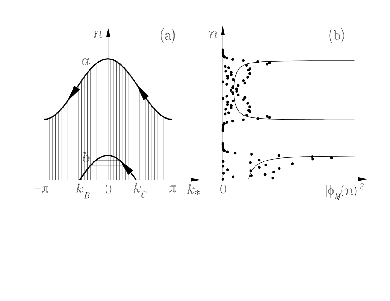
FIG. 1.: (a) The bulk (curve $a$) and the edge (curve $b$) classical trajectories of electrons in the phase space $(n,k_{*})$. The coordinate $n$ is confined between $(E_{M}\pm t)/\Omega$ for the bulk state and between $(E_{M}+t)/\Omega$ and 0 for the edge state. (b) Solid lines: Classical probability distributions for the two trajectories shown in panel (a). Dots: Quantum probability distributions $|\phi_{M}(n)|^{2}$ of the two wave functions corresponding to the two trajectories.

When $t\gg\Omega$, integral (6) with $\varphi_{M}(k)$ from Eq. (8) can be taken by the method of steepest descent in the vicinity of the points $k_{*}$ where the derivative in $k$ of the phase of the integrand vanishes:

$$n=\xi(k_{*},E_{M})=(E_{M}+2t\cos k_{*})/\Omega.$$ (11)

Eq. (11) can be interpreted as the classical conservation law of the kinetic, $-2t\cos k_{*}$, and potential, $n\Omega$, energies of electron. If the coordinate $n$ belongs to the classically allowed region $[(E_{M}-2t)/\Omega,(E_{M}+2t)/\Omega]$, then $k_{*}$ is real; otherwise, $k_{*}$ is complex. Real solutions of Eq. (11) describe classical electron trajectories in the phase space $(n,k_{*})$. When $E_{M}>2t$, the trajectory lies entirely within the region $n>0$ and does not cross the boundary of the crystal at $n=0$ (curve $a$ in Fig. 1(a)). When $-2t<E_{M}<2t$, the trajectory reaches the edge (curve $b$ in Fig. 1(a)). These two types of classical trajectories correspond to the bulk and the edge quantum states of electrons. The classical motion is periodic both for the bulk trajectory, because the end points $k_{*}=\pm\pi$ correspond to the same state, and for the edge trajectory, because elastic reflection at point $k_{B}$ reverses the sign of $k_{*}$ and transfers electron back to point $k_{C}$. Thus, we expect the WKB quantization condition to apply in both cases:

$$\int\xi(k,E_{M})\,dk=2\pi(M+\gamma),$$ (12)

where $-1<\gamma\leq 0$ is a constant, and the integral represents the phase space area enclosed by the classical trajectory. For the bulk and the edge trajectories $a$ and $b$ in Fig. 1(a), these areas are shaded vertically and horizontally. Contrary to Ref. [9], we find well-defined WKB quantization areas for both the bulk and the edge trajectories.

To derive quantization condition (12) for our model formally and to find the constant $\gamma$, we need to apply the boundary conditions properly. Integral (6) with $\varphi_{M}(k)$ given by Eq. (9) converges only if the ends of the integration contour extend to infinity within the shaded areas in Fig. 2, where ${\rm Im}\sin k<0$, and $\varphi_{M}(k)$ tends to zero at infinity. The right boundary condition in real space, $\phi_{M}(n)\rightarrow 0\;\;{\rm at}\;\;n\rightarrow+\infty,$ is satisfied provided the contour of integration starts in area $I$ and ends in area $II$ in Fig. 2. Indeed, in the classically inaccessible region $n\rightarrow+\infty$, solutions of Eq. (11) are imaginary. One of them, $k_{A}=i\,{\rm arccosh}(n^{\prime}\Omega/2t)$, where $n^{\prime}=n-E_{M}/\Omega$, is represented by point $A$ in Fig. 2. The contour of integration connects regions $I$ and $II$ by passing through point $A$. Taking integral (6) in the vicinity of point $A$ along the direction of steepest descent, which is parallel to the real axis of $k$ in this case, we find:

$$\phi_{M}(n)\approx\exp\{-n^{\prime}[\ln(n^{\prime}\Omega/t)-1]\}/\sqrt{2\pi n^{\prime}},$$ (13)

which does satisfy the right boundary condition.

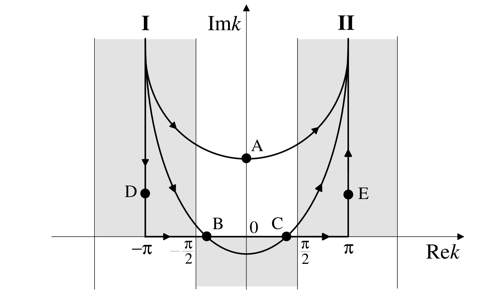
FIG. 2.: Complex plane of $k$. Thick lines show the contours of integration in Eq. (6) for three different positions of the coordinate $n$.

Now let us calculate $\phi_{M}(n)$ in the classically accessible region. In this case, solutions of Eq. (11), represented by points $B$ and $C$ in Fig. 2, are real: $k_{C}=-k_{B}=\arccos(n^{\prime}\Omega/2t)$. The contour of integration connects regions $I$ and $II$ by passing through points $B$ and $C$:

$$\phi_{M}(n) = \left(e^{ink_{B}-i\pi/4}+e^{ink_{C}+i\pi/4-i\int_{k_{B}}^{k_{C}}\xi(k^{\prime},E_{M})\,dk^{\prime}}\right)$$ (15)

$$\times\varphi_{M}(k_{B})/\sqrt{2\pi}\sqrt[4]{(2t/\Omega)^{2}-n^{\prime 2}}.$$

The factors $\exp(\mp i\pi/4)$ appear in Eq. (15), because the directions of steepest descent for points $B$ and $C$ are at the angles $\mp\pi/4$ to the real axis of $k$. The integral from $k_{B}$ to $k_{C}$ in Eq. (15) reflects the change of function (8) between points $B$ and $C$. For the edge states, the point $n=0$ is classically accessible. To satisfy the left boundary condition (5), the first line in Eq. (15) must vanish at $n=0$. This generates quantization condition (12) with $\gamma=-1/4$ for the edge states:

$$\int_{-\arccos(-E_{M}/2t)}^{\arccos(-E_{M}/2t)}\xi(k,E_{M})\,dk=2\pi\left(M-\frac{1}{4}\right).$$ (16)

Substituting Eq. (10) into Eq. (16) gives a transcendental equation on $E_{M}$, which has the following explicit solution for the states on the very edge with $M\ll t/\Omega$:

$$E_{M}=t\{-2+[(3\pi\Omega/2t)(M-1/4)]^{2/3}\}.$$ (17)

The total number of the edge states is $n_{\rm edge}=2t/\Omega$. Eqs. (16) and (17) are similar to the edge states quantization equations for a closed Fermi surface [19].

In the classically inaccessible region $n<(E_{M}-2t)/\Omega$, solutions of Eq. (11), represented by points $D$ and $E$ in Fig. 2, are complex: $k_{D,E}=\mp\pi+i\,{\rm arccosh}(-n^{\prime}\Omega/2t)$. The contour of integration connects regions $I$ and $II$ by passing through points $D$ and $E$:

$$\phi_{M}(n)=(-i)\left[1-\exp\left(-i\int_{k_{D}}^{k_{E}}\xi(k^{\prime},E_{M})\,dk^{\prime}\right)\right]$$ (18)

$$\times\exp\{-n^{\prime}[{\rm arccosh}(-n^{\prime}\Omega/2t)+i\pi]\}$$ (19)

$$\times\exp[-\sqrt{n^{\prime 2}-(2t/\Omega)^{2}}]/\sqrt{2\pi}\,\sqrt[4]{n^{\prime 2}-(2t/\Omega)^{2}}.$$ (20)

The integral between $k_{D}$ and $k_{E}$ in Eq. (20) proceeds along the horizontal line $[-\pi,\pi]$ and the vertical lines $[k_{D},-\pi]$ and $[\pi,k_{E}]$ (see Fig. 2); however, the integrals along the vertical lines cancel. To satisfy the left boundary condition, Eq. (5) for a semi-infinite crystal or $\phi_{M}(n)\rightarrow 0$ at $n\rightarrow-\infty$ for an infinite one, the first line in Eq. (20) must vanish. This generates quantization condition (12) with $\gamma=0$ for the bulk states:

$$\int_{-\pi}^{\pi}\xi(k,E_{M})\,dk=2\pi M.$$ (21)

Substituting Eq. (10) into Eq. (21), we recover the Wannier-Stark ladder [14] for the bulk states energies:

$$E_{M}=M\Omega.$$ (22)

When Eq. (22) applies, the function $\varphi_{M}(k)$ in Eq. (9) is periodic: $\varphi_{M}(k)=\varphi_{M}(k+2\pi)$, thus integral (6) can be taken only from $-\pi$ to $\pi$, because the integrals along the vertical portions of the integration contour cancel. In this case, the bulk wave functions are expressed in terms of the Bessel functions $J$ of an integer order: $\phi_{M}(n)=J_{n-M}(2t/\Omega)$.

In all cases, as follows from Eqs. (6) and (9) with the contours of integration shown in Fig. 2, the electron wave functions

$$\phi_{M}(n) = \int\frac{dk}{2\pi}\exp\left(ink-i\frac{E_{M}k+2t\sin k}{\Omega}\right)$$ (23)

$$= J_{n-E_{M}/\Omega}(2t/\Omega)$$ (24)

are nothing but the Bessel functions of a general order $n-E_{M}/\Omega$ in the Sommerfeld representation [20]. The quantized value of the energy $E_{M}$ is determined by the boundary condition (5):

$$J_{-E_{M}/\Omega}(2t/\Omega)=0.$$ (25)

The quantization condition in the form (25) was found in Ref. [15]. As shown in Appendix, Ref. [10] would have obtained the same Eq. (25), if mathematical errors were not made there.

The electron wave functions can be expressed in terms of the Bessel functions (24) only when $\varepsilon_{\perp}(k)=-2t\cos k$ in Eqs. (10) and (8), which corresponds to the electron tunneling between the nearest neighboring chains. Proper description of the Bechgaard salts requires to take into account higher harmonics of the transverse dispersion law of electron, such as $-2t^{\prime}\cos 2k$, which corresponds to the electron tunneling between the next-nearest neighboring chains [21]. The WKB method described in this section is still applicable for an arbitrary transverse dispersion law $\varepsilon_{\perp}(k)$, but the wave functions are not the Bessel functions any more.

III Numerical solution and discussion

To verify the semiclassical results, we solve Eq. (2) for a finite number of chains $n_{\rm max}=150\gg n_{\rm edge}=2t/\Omega=25$ by numerical diagonalization of the Hamiltonian

$$\hat{\cal H}=\left(\begin{array}[]{cccccc}\Omega&-t&0&0&\cdots&0\\ -t&2\Omega&-t&0&\cdots&0\\ 0&-t&3\Omega&-t&\cdots&0\\ \vdots&\vdots&\ddots&\ddots&\ddots&\vdots\\ 0&0&\cdots&-t&(n_{\rm max}-1)\Omega&-t\\ 0&0&\cdots&0&-t&n_{\rm max}\Omega\end{array}\right).$$ (26)

The quantum probability distributions $|\phi_{M}(n)|^{2}$ of two eigenfunctions of Hamiltonian (26) (the dots in Fig. 1(b)) agree with the classical probability distributions (the solid lines in Fig. 1(b)) of the corresponding bulk and edge trajectories shown in Fig. 1(a). The classical probability distributions are proportional to the square of Eq. (15) and are equal to $2/Tv_{y}$, where $v_{y}=2t\sin k_{*}/\hbar\propto 1/\sqrt{(2t)^{2}-(n^{\prime}\Omega)^{2}}$ is the velocity and $T=\oint dn/v_{y}$ is the period of classical motion. The numerically calculated eigenvalues $E_{M}$ of Hamiltonian (26), shown in Fig. 3(a), agree with the semiclassical energies found from Eqs. (22), (16), and (10) within less than 1%. As Fig. 3(a) demonstrates, the energy levels are uniformly spaced in the bulk (see Eq. (22)) with the energy $\Omega$ (3) proportional to the magnetic field, but the spacing is different and not uniform near the edges. In agreement with Eq. (17), the spacing of the levels near the edges is sublinear ($E_{M}\propto{\rm const}+M^{2/3}$), and the extremal energy levels with $M=1$ and $M=n_{\rm max}$ are displaced relative to the linear extrapolation of the bulk law (22) by the amount $\Delta E\approx\mp 2t$.

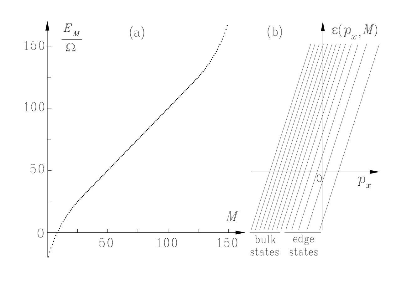
FIG. 3.: (a) Eigenenergies $E_{M}$ of Hamiltonian (26) found by numerical diagonalization in the case $n_{\rm max}=150$ and $n_{\rm edge}=2t/\Omega=25$. (b) Electron dispersion law $\varepsilon(p_{x},M)$ (4). Only the branches with $M=1,6,11,\ldots,61$ are shown.

Transitions between the energy levels $E_{M}$ in an external ac electromagnetic field constitute the cyclotron resonance. Because the penetration depth in metals is short, we expect the energies (17) of the edge states to show up in the surface impedance, as in conventional metals [19]. The edge states were neglected in the theory of the cyclotron resonance in Q1D conductors [8].

The complete, transverse and longitudinal, dispersion law (4) is shown in Fig. 3(b). It consists of discrete branches, each having a continuous linear dispersion in $p_{x}$. The Fermi momenta of the branches,

$$p_{F}^{(M)}=-E_{M}/v_{F}$$ (27)

are defined as the points where the energy $\varepsilon(p_{x},M)$ (4) vanishes. The Fermi momenta of the bulk states are spaced uniformly with the distance $G=\Omega/v_{F}=ebH/c$, but the spacing is different and not uniform near the edge. This may have important consequences for the FISDW state. The FISDW couples the $+P_{F}$ electrons in the eigenstate $M$ with the $-P_{F}$ electrons in the eigenstate $M-N$ [5]. As long as Eq. (22) applies, the FISDW wave vector $Q_{x}=2P_{F}-NG$ exactly matches the difference between the Fermi momenta of these states and opens an energy gap in their spectrum. $N$ branches of the $+P_{F}$ electrons at one edge of the crystal and $N$ branches of the $-P_{F}$ electrons at the other edge remain gapless, because they have no partners to couple with [5]. Even though these $2N$ modes are gapless, electric current is not dissipated, because the modes are chiral, and the Hall conductivity is quantized: $\sigma_{xy}=2Ne^{2}/h$, where $h$ is the Planck constant [5]. However, the wave vector $Q_{x}=2P_{F}-NG$ does not match the Fermi momenta (27) near the edges, where their spacing is not uniform. Thus, gapless electron pockets should exist there and cause dissipation in the QHE regime. The size of the pockets may be reduced if $Q_{x}$ adjusts to the spacing of the edge states. The energetics involved in the latter effect requires a separate study.

IV Equilibrium currents and magnetization

Since the transverse eigenfunctions $\phi_{M}(n)$ are real, they carry no electric current across the chains. The current carried by eigenstates (1) along the chains is

$$j^{\pm}_{p_{x},M}(n)=e\left(\pm v_{F}-\frac{eA_{x}(n)}{cm_{e}}\right)|\phi^{\pm}_{M}(n)|^{2},$$ (28)

where $m_{e}$ is the electron band mass, and the signs $\pm$ refer to the $\pm P_{F}$ electrons. To find the total current $I$ at the chain $n$, we sum Eq. (28) over $M$ and integrate over $p_{x}$ with the Fermi distribution function (at zero temperature):

$$I(n) = 2e\sum_{M=1}^{n_{\rm max}}\int\limits_{-P_{F}-p_{F}^{(M)}}^{P_{F}+p_{F}^{(M)}}\frac{dP_{x}}{2\pi\hbar}\,(\pm v_{F})|\phi^{\pm}_{M}(n)|^{2}$$ (30)

$$-\frac{2e^{2}A_{x}(n)}{cm_{e}}\sum_{M=1}^{n_{\rm max}}\int\limits_{-P_{F}-p_{F}^{(M)}}^{P_{F}+p_{F}^{(M)}}\frac{dP_{x}}{2\pi\hbar}\,|\phi^{\pm}_{M}(n)|^{2},$$

where the factor 2 comes from the spin of electrons. It is understood that the wave functions $\phi^{+}_{M}(n)$ and $\phi^{-}_{M}(n)$ should be used when the integration over $P_{x}$ is close to $+P_{F}$ and $-P_{F}$, and some interpolating functions should be used for the intermediate values of $P_{x}$. The result does not depend on the contributions far from the Fermi surface.

Taking into account that

$$|\phi^{+}_{M}(n)|=|\phi^{-}_{M}(n)|,$$ (31)

we find that the integral $\int_{-P_{F}}^{P_{F}}dP_{x}$ in Eq. (30) vanishes. The only nonzero contribution to this term comes from the deviations $p_{F}^{(M)}$ (27) from the 1D Fermi momenta $\pm P_{F}$:

$$\frac{e}{\pi\hbar}\sum_{M=1}^{n_{\rm max}}-E^{+}_{M}|\phi^{+}_{M}(n)|^{2}+E^{-}_{M}|\phi^{-}_{M}(n)|^{2}.$$ (32)

Taking into account that the eigenfunctions $\phi^{+}_{M}(n)$ form a complete basis of Hamiltonian (26) and using the relations $E^{+}_{M}=-E^{-}_{M}$ and Eq. (31), we find that Eq. (32) can be rewritten as

$$-\frac{2e}{\pi\hbar}\langle n|\hat{\cal H}|n\rangle=-\frac{2e}{\pi\hbar}n\Omega,$$ (33)

where $\langle n|\hat{\cal H}|n\rangle$ are the diagonal matrix elements of Hamiltonian (26).

Using Eq. (31), the term (30) can be written as

$$\frac{2eA_{x}(n)}{cm_{e}}\int_{-P_{F}}^{P_{F}}\frac{dP_{x}}{2\pi\hbar}\sum_{M=1}^{n_{\rm max}}|\phi^{\pm}_{M}(n)|^{2}.$$ (34)

Taking into account the completeness relation $\sum_{M}|\phi^{\pm}_{M}(n)|^{2}=1$ and integrating over $P_{x}$, we transform Eq. (34) into

$$\frac{2eA_{x}(n)v_{F}}{c\pi\hbar}=\frac{2en\Omega}{\pi\hbar}.$$ (35)

The two terms (33) and (35) cancel each other, so that the total electric current on any chain $n$ is zero:

$$I(n)=0.$$ (36)

Because the current vanishes everywhere including the edges, there is no orbital magnetization (and no de Haas-van Alphen oscillations proposed in Refs. [9, 10]) in a Q1D metal in a magnetic field. Experimentally, no magnetization was found in the Bechgaard salts in the metallic state [22] (unlike in the FISDW state, where energy gaps exist in the electron spectrum).

V Magnetization in the case of quadratic dispersion law

In the previous section, we found that orbital magnetization of the system vanishes identically. That is a consequence of the linearized longitudinal energy dispersion law of electrons in our model. However, for a nonlinear dispersion law, magnetization is not necessarily zero. We can crudely estimate the change in the bulk free energy per one electron at zero temperature generated by an applied magnetic field, $\Delta F$, in the following way. $\Delta F$ must vanish when $H\to 0$ and when $t\to 0$. (When $t=0$, the magnetic field has no orbital effect on 1D uncoupled chains.) Because $\Delta F$ does not depend on the signs of $H$ and $t$, it should be quadratic in $\Omega=ebHv_{F}/c$ and $t$ in the lowest order. To achieve the dimensionality of energy, we need to divide the expression by a power of the Fermi energy $\varepsilon_{F}=P_{F}v_{F}/2$. In this way, we find

$$\Delta F\sim t^{2}\Omega^{2}/\varepsilon_{F}^{3}.$$ (37)

Magnetization is obtained by differentiating Eq. (37) in $H$.

It is difficult to calculate $\Delta F$ explicitly in the case of a weak magnetic field: $\Omega\ll t\ll\varepsilon_{F}$. In the semiclassical (WKB) approximation, the bulk free energy of a Q1D metal does not depend on the magnetic field, even if the longitudinal dispersion law is nonlinear, as long as the Fermi surface is open, and the electron energy spectrum is continuous, not quantized [13]. This result is related to the Bohr-van Leeuwen theorem, which states that partition function in classical statistical mechanics does not depend on magnetic field. Thus, in order to obtain a nonzero $\Delta F$, it is necessary to go beyond the WKB approximation, which is difficult.

On the other hand, we can easily calculate $\Delta F$ in case of a strong magnetic field: $t\ll\Omega\ll\varepsilon_{F}$, although this case may not correspond to the Bechgaard salts in realistic magnetic fields. In this case, the transverse tunneling amplitude $t$ can be treated as a small perturbation to the energy spectrum. The second order correction to the total energy of the system per one electron at zero temperature due to a perturbation $V$ is given by the following expression:

$$\Delta F^{(2)}=\frac{1}{N_{e}}\sum_{\alpha\>(\varepsilon_{\alpha}<\varepsilon_{F})\atop\beta\>(\varepsilon_{\beta}>\varepsilon_{F})}\frac{\langle\alpha|V|\beta\rangle\langle\beta|V|\alpha\rangle}{\varepsilon_{\alpha}-\varepsilon_{\beta}},$$ (38)

where $N_{e}$ is the total number of electrons, and the sum is taken over the energy eigenstates below and above the Fermi energy, labeled by the indices $\alpha$ and $\beta$, respectively. Treating the transverse tunneling amplitude $t$ as the perturbation $V$ and taking into account that its matrix elements change the longitudinal momentum $p_{x}$ by $\pm G$: $\langle\alpha_{k^{\prime}_{x},M^{\prime}}|V|\beta_{k_{x},M}\rangle=-t\,\delta_{M^{\prime},M\pm 1}\,\delta(k^{\prime}_{x}-k_{x}\mp G)$, we find that the sum in Eq. (38) is restricted to an interval of the width $G$ in the vicinity of the Fermi momentum:

$$\delta F^{(2)}=\frac{4t^{2}}{\rho_{e}}\int_{-G}^{0}\frac{dp_{x}}{2\pi\hbar}\,\frac{1}{\varepsilon_{\parallel}(p_{x})-\varepsilon_{\parallel}(p_{x}+G)}.$$ (39)

In Eq. (39), the factor of 4 accounts for the two Fermi points and two spin orientations, and $\rho_{e}=4k_{F}/2\pi$ is the electron concentration per one chain. Using the quadratic longitudinal dispersion law $\varepsilon_{\parallel}(p_{x})=(P_{F}+p_{x})^{2}/2m_{e}$, where $m_{e}$ is the effective electron mass, we find:

$$\Delta F^{(2)} = -\frac{4t^{2}}{\rho_{e}}\int_{-G}^{0}\frac{dp_{x}}{2\pi\hbar}\,\frac{m_{e}}{G(P_{F}+p_{x}+G/2)}$$ (40)

$$= -\frac{t^{2}}{\Omega}\ln\left(\frac{P_{F}+G/2}{P_{F}-G/2}\right).$$ (41)

Expanding Eq. (41) in the small parameter $G/P_{F}=\Omega/2\varepsilon_{F}$ and keeping the first two nonvanishing terms, we find:

$$\Delta F^{(2)}=-\frac{t^{2}}{2\varepsilon_{F}}-\frac{t^{2}\Omega^{2}}{96\varepsilon_{F}^{3}}+\ldots$$ (42)

The first term in Eq. (42) coincides with the second-order correction due to the electron tunneling between the chains in the absence of magnetic field. Only this, magnetic-field-independent term is obtained, if the longitudinal dispersion law is linearized in Eq. (39). The second term in Eq. (42) appears due to nonlinearity of the dispersion law and reproduces the result of dimensional analysis (37) up to a numerical factor. Its negative sign indicate paramagnetism. However, because the carriers in (TMTSF)₂X are holes with a negative $m_{e}$, the orbital response would be diamagnetic in these materials.

VI Conclusions

In conclusion, the energy of either a bulk or an edge electron state in a Q1D metal is the sum of two terms (4), one of which has a continuous spectrum and the other discrete. The discrete part of the electron energy is determined by the semi-infinite Wannier-Stark equation (2). We have solved the semi-infinite Wannier-Stark problem semiclassically and numerically. The WKB quantization condition (12) of the electron phase space area (Fig. 1(a)) determines the energies of the edge states with the constant $\gamma=-1/4$ (16) and the bulk states with $\gamma=0$ (21). The energies are spaced uniformly in the bulk, but not near the edges (see Fig. 3(a) and Eqs. (22) and (17)). These results may be important for the cyclotron resonance and the QHE in the Bechgaard salts, as well as the finite-size GaAs-Ga_1-xAl_xAs superlattices in an electric field. We have demonstrated explicitly that the equilibrium electric currents vanish both at the edges and in the bulk, so no orbital magnetization is expected in a Q1D metal in a magnetic field in the approximation of linearized longitudinal energy dispersion law of electrons. We have also estimated the magnitude of orbital magnetization for the quadratic longitudinal dispersion law.

Appendix

In this Appendix, we use the notation of Ref. [10]. Eq. (8) of Ref. [10]:

$$\frac{1}{2}\pi MJ_{\nu}(M)J_{1-\nu}(M)=\sin(\pi\nu),$$ (43)

can be simplified by using identity (9.1.15) from Ref. [23]:

$$J_{\nu+1}(M)J_{-\nu}(M)+J_{\nu}(M)J_{-\nu-1}(M)=-\frac{2\sin(\pi\nu)}{\pi M}.$$ (44)

Substituting Eq. (44) into Eq. (43), we find:

$$J_{\nu}(M)[J_{-\nu+1}(M)+J_{-\nu-1}(M)]=-J_{\nu+1}(M)J_{-\nu}(M).$$ (45)

Using the recurrence relation (9.1.27) of Ref. [23]:

$$J_{\nu+1}(M)+J_{\nu-1}(M)=\frac{2\nu}{M}J_{\nu}(M),$$ (46)

in Eq. (45), we find:

$$J_{-\nu}(M)\left[\frac{2\nu}{M}J_{\nu}(M)-J_{\nu+1}(M)\right]=0.$$ (47)

Using the recurrence relation (46) in Eq. (47) again, we find:

$$J_{-\nu}(M)J_{\nu-1}(M)=0.$$ (48)

Eq. (48) is satisfied if either

$$J_{-\nu}(M)=0,$$ (49)

or

$$J_{\nu-1}(M)=0.$$ (50)

Eq. (49) is the same as our energy quantization condition Eq. (25). Eq. (50) describes unphysical electron states located outside of the crystal ($m\leq 0$) and should be discarded. The two sets of eigenvalues, (49) and (50), are completely decoupled and do not repel when cross. Thus there should be no gaps in Fig. 2 of Ref. [10], no the fractional interference between the two set of the energy levels, and no diamagnetic oscillations. Contrary to the explicit transformation given above, the two sets of eigenvalues come out coupled via a constant $A$ in Eq. (10) of Ref. [10]. We conclude that there must be an error in the “rather boring calculations” mentioned between Eqs. (9) and (10) and leading from Eq. (8) to Eq. (10) in Ref. [10]. The conclusions following Eq. (10) in Ref. [10] are invalid because of the error in this equation.

REFERENCES

- [1] E-mail yakovenk@physics.umd.edu.
- [2] TMTSF is tetramethyltetraselenafulvalene and X represents a monovalent inorganic anion.
- [3] P. M. Chaikin, J. Phys. I (Paris), 6, 1875 (1996).
- [4] P. Lederer, J. Phys. I (Paris), 6, 1899 (1996).
- [5] V. M. Yakovenko and H.-S. Goan, J. Phys. I (Paris), 6, 1917 (1996).
- [6] J. T. Chalker and A. Dohmen, Phys. Rev. Lett. 75, 4496 (1995).
- [7] L. Balents and M. P. A. Fisher, Phys. Rev. Lett. 76, 2782 (1996).
- [8] L. P. Gor’kov and A. G. Lebed’, Phys. Rev. Lett. 71, 3874 (1993).
- [9] M. Ya. Azbel and P. M. Chaikin, Phys. Rev. Lett. 59, 582 (1987).
- [10] M. Ya. Azbel, Phys. Rev. Lett. 64, 1282 (1990).
- [11] T. Osada and N. Miura, Solid State Commun. 69, 1169 (1989).
- [12] M. Ya. Azbel, Phys. Rev. B 39, 6241 (1989).
- [13] I. M. Lifshits, M. Ya. Azbel, and M. I. Kaganov, Electron Theory of Metals (Consultants Bureau, New York, 1973).
- [14] G. H. Wannier, Phys. Rev. 117 432 (1960).
- [15] H. Fukuyama, R. A. Bari, and H. C. Fogedby, Phys. Rev. B 8, 5579 (1973).
- [16] G. C. Stey and G. Gusman J. Phys. C 6, 650 (1973).
- [17] E. E. Mendez and G. Bastard, Phys. Today, June, p. 34 (1993).
- [18] L. D. Landau and E. M. Lifshitz, Quantum Mechanics: Non-relativistic Theory (Pergamon Press, Oxford, 1991), Appendix B.
- [19] R. E. Prange and T.-W. Nee, Phys. Rev. 168 779 (1968); M. S. Khaǐkin, Sov. Phys. Usp. 17, 785 (1969).
- [20] A. F. Nikiforov and V. B. Uvarov, Special Functions of Mathematical Physics (Birkhäuser, Boston, 1988) Ch. III.13; Handbook of Applied Mathematics, edited by C. E. Pearson (Van Nostrand Reinhold Co, New York, 1983) Ch. 7.4.4.
- [21] G. Montambaux, M. Héritier, and P. Lederer, Phys. Rev. Lett. 55, 2078 (1985); D. Zanchi and G. Montambaux, Phys. Rev. Lett. 77, 366 (1996).
- [22] M. J. Naughton et al., Phys. Rev. Lett. 55, 969 (1985); X. Yan et al., Phys. Rev. B 36, 1799 (1987); R. V. Chamberlin et al., Phys. Rev. Lett. 60, 1189 (1988).
- [23] Handbook of Mathematical Functions, ed. by M. Abramowitz and I. Stegun (Dover, New York, 1972).