The two-dimensional Anderson model of localization with random hopping

Abstract

We examine the localization properties of the 2D Anderson Hamiltonian with off-diagonal disorder. Investigating the behavior of the participation numbers of eigenstates as well as studying their multifractal properties, we find states in the center of the band which show critical behavior up to the system size $N=200\times 200$ considered. This result is confirmed by an independent analysis of the localization lengths in quasi-1D strips with the help of the transfer-matrix method. Adding a very small additional onsite potential disorder, the critical states become localized.

I Introduction

Nearly forty years have passed since Anderson’s [1] first suggestion of a disorder-induced metal-insulator transition (MIT), and yet the localization problem remains at the center of much interest.

For non-interacting electrons, a highly successful approach was put forward in 1979 by Abrahams et al. [2]. This “scaling hypothesis of localization” suggests that an MIT exists for non-interacting electrons in three dimensions (3D) at zero magnetic field $B$ and in the absence of spin-orbit coupling. Much further work has subsequently supported these scaling arguments both analytically and numerically [3, 4]. In 1D and 2D, the same hypothesis shows that there are no extended states and thus no MIT. However, since 2 is the lower critical dimension of the localization problem [5], the 2D case is in a sense “close” to 3D: states are only marginally localized for weak disorder and a small magnetic field or spin-orbit coupling can lead to the existence of extended states and thus an MIT. Consequently, the localization lengths of a 2D system with potential disorder can be quite large [6, 7] so that in numerical approaches one can always find a localization-delocalization transition when decreasing either system size for fixed disorder or disorder for fixed system size [8].

The role played by many-particle interactions is much less understood [9]. Even for disordered quantum many-body systems in 1D, no entirely consistent picture exists [10]. Thus recent experimental results [11], which indicate the existence of an MIT in certain 2D electron gases at $B=0$, are a challenge to our current understanding. In the samples considered, the Coulomb interaction is estimated to be much larger than the Fermi energy [11] and so the observed MIT may be due to an interaction-driven enhancement of the conductivity. A recent reevaluation [12] of the principles of scaling theory shows that these experimental results do in fact not violate general scaling principles. However, it is not yet clear that this transition does indeed correspond to an MIT since other recent arguments [13] suggest that the transition might be understood as an insulator-superconductor transition.

Most numerical approaches to the localization problem use the standard tight-binding Anderson Hamiltonian with onsite potential disorder. Characteristics of the electronic eigenstates are then investigated by studies of participation numbers [14] obtained by exact diagonalization, multifractal properties [15, 16], level statistics [17] and many others. Especially fruitful is the transfer-matrix method (TMM) [7] which allows a direct computation of the localization lengths and further validates the scaling hypothesis by a numerical proof of the existence of a one-parameter scaling function.

In the present work, we have reconsidered a variant of the Anderson model in which also the nearest-neighbor hopping elements are allowed to be randomly distributed. Prior to the advent of the scaling hypothesis, Thouless-type arguments showed the possibility of much larger localization lengths in such a 2D system [18] as compared to the case with potential disorder only. Thus, motivated in part by the above mentioned experimentally observed transition in 2D systems at $B=0$, this model provides a good starting point for a search of 2D states which, perhaps, need not be localized. Another motivation is provided by the 2D random magnetic flux model (RFM) [19, 20], in which the hopping elements are chosen to be of unit modulus but with a random phase representing a random magnetic field penetrating the 2D plane. Although much effort has been dedicated towards the RFM, no definite picture exists and results range from a complete absence of diffusion to the prediction of extended states near the band center [19]. Our random hopping model may be viewed as a RFM with phase fixed at zero but random modulus.

In the present paper, we will present a comprehensive numerical study of the 2D Anderson model with random hopping. In section II we introduce the model and notation. In order to get a first insight into the differences and the similarities of the random hopping and the potential disorder case, we look at the eigenstates and their Fourier transforms in section III. We calculate the density of states (DOS) in section IV and show an unusual feature in the band center $E=0$. In section V we then study participation numbers and multifractal properties, respectively. A scaling analysis of the participation numbers suggests that the states at $E=0$ for system sizes up to $N=200\times 200$ behave similar to critical states at the MIT in the 3D Anderson model. We confirm this result by the TMM together with the one-parameter finite-size-scaling (FSS) analysis [7] in section VI: the states at $E=0$ show critical behavior up to a strip width $M=180$. However, already a very small additional onsite potential disorder destroys the criticality. We summarize and conclude in section VII.

II The Model

The 2D Anderson Hamiltonian is given as

$$H=\sum_{i}^{N}\epsilon_{i}|i\rangle\langle i|+\sum_{i\neq j}^{N}t_{ij}|i\rangle\langle j|.$$ (1)

The sites $i=(n,m)$ form a regular square lattice of size $N=L\times L$ and, unless stated otherwise, we will always use periodic boundary conditions. The onsite potential energies $\epsilon_{i}$ are taken to be randomly distributed in the interval $[-W/2,W/2]$. The transfer integrals $t_{ij}$ are restricted to nearest-neighbors and chosen to be randomly distributed in the interval $[c-w/2,c+w/2]$. Thus $c$ represents the center and $w$ the width of the off-diagonal disorder distribution. We set the energy scale by keeping $w=1$ fixed, except for the cases of pure diagonal disorder where the hopping elements are constant ($w=0$ and $c=1$). For $c\rightarrow\infty$, the off-diagonal disorder width $w$ is negligible compared to its mean, and we get the usual Anderson model; when additionally $W$ remains finite for $c\rightarrow\infty$, the system becomes ordered. On the other hand, for $c\leq 0.5$, individual hopping elements may be zero and transport will be hindered more strongly. This will give a more pronounced tendency towards localization.

We note that for the case of purely off-diagonal disorder ($W=0$) we have an exact particle-hole symmetry in the band such that for any eigenstate with energy $E_{j}>0$, there is also an eigenstate with energy $E_{j^{\prime}}=-E_{j}$. In the usual Anderson model with $W>0$ and $w=0$, this exact symmetry is only recovered in the limit of infinite system size $N\rightarrow\infty$.

Our numerical approach to the present model is based on (i) an exact diagonalization of the respective secular matrices by means of the Lanczos algorithm [21], and (ii) a recursion form for the Schrödinger equation corresponding to the Hamiltonian (1) which provides the starting point for the TMM of section VI.

III Looking at the wave functions

A Probability density in real space

Let us start our investigation of the Hamiltonian (1) by simply looking at some typical eigenstates $\phi_{j}(n,m)$ obtained by exact diagonalization. For small off-diagonal disorder $c>0.5$, the ordered system is only slightly perturbed and we expect the weakest localization of the wave function to occur at the band center $E=0$ just as for purely diagonal disorder $W$. In Fig. 1, we show the spatial dependence of the probability density of the wave function at $E=0$ for various values of $c$. For $c>0.5$, the probability density is rather homogeneously distributed over all $N$ sites. For comparison, we also include 3 examples of an analogous plot for purely diagonal disorder ($w=0$), showing a similarly homogeneous distribution for small $W$. E.g. the probability density plot at $c=2$ $(W=0)$ is very similar to the plot for $W=1$ ($w=0$). With decreasing $c\leq 0.5$ the wavefunctions become concentrated in certain areas, indicating a tendency towards localization. Moreover, differences between diagonal and off-diagonal disorder become noticeable: systems with purely off-diagonal disorder exhibit large site-to-site probability density fluctuations resulting in characteristic chess board patterns, whereas in the systems with diagonal disorder separate areas of large probability appear. We also see from Fig. 1 that $c=0$ does not seem to correspond to the strongest localization. Rather, the strongest “curdling” [15] of a state occurs at $c\approx 0.25$. For purely diagonal disorder, it is well-known that the localization is strongest for states with energies close to the band edges. In agreement, we have found, but refrain from showing corresponding plots here, that with increasing energy towards the band edges the patterns of probability density for purely off-diagonal disorder tend to be more localized and become thus again similar to those for diagonal disorder.

B Probability density in Fourier space

According to the usual connection between real and Fourier space, extended states in real space appear localized in Fourier space, whereas localized states in real space appear extended in Fourier space. Furthermore, eigenstates of the disordered system at energy $E$ are superpositions of eigenstates of the ordered system at energies $E^{\prime}=E\pm\Delta E(w,W)$, where $\Delta E(w,W)$ represents an energy level broadening due to the disorder. For weak disorder the expansion coefficients of this superposition are approximately equal for states with small $\Delta E$. Interpreting $E$ as the Fermi energy, an eigenstate of the weakly disordered system in Fourier space should therefore exhibit the Fermi surface (FS). Consequently, we can study what happens to the FS upon increasing the disorder. The 2D Fourier transform of the state $\phi_{j}(n,m)$ is defined as

$$\phi_{j}(k_{n},k_{m})=\sum_{n}^{L}\sum_{m}^{L}\phi_{j}(n,m)\exp(\frac{2\pi ik_{n}n}{L})\exp(\frac{2\pi ik_{m}m}{L}).$$ (2)

In Fig. 2, we show probability densities of Fourier transformed wavefunctions $\phi_{j}(k_{n},k_{m})$. As expected, weak diagonal and off-diagonal disorder produces states that appear localized in Fourier space and reproduce the FS of the 2D tight-binding model with nearest-neighbor hopping on a square lattice. As examples consider the probability density plot at $c=2$ ($W=0$) and the plot for $W=1$ ($w=0$). With decreasing $c$ the states smear out, but the FS can still be seen. Again, the behavior is qualitatively similar for both purely off-diagonal and diagonal disorder as can be seen by comparing the probability densities for $c=0.5$ ($W=0$) and $W=5$ ($w=0$) in Fig. 2. The difference between the two types of disorder appears only for $c<0.5$. E.g., states for off-diagonal disorder $c=0$ appear completely delocalized in Fourier space, whereas for strong diagonal disorder $W=8$ there is still a remnant of the FS. This feature persists even at higher energies, suggesting different localization properties of states in systems with off-diagonal disorder characterized by small $c$.

IV Density of States

In Fig. 3, we show the scaled DOS for off-diagonal disorder obtained by averaging over many samples of size $N=96\times 96$. The off-diagonal disorder strengths are $c=0$, $0.5$, and $2$ with $E_{max}=1.27$, $2.63$ and $8.24$, respectively. For a 2D ordered system, the DOS has a logarithmic singularity at the band center $E=0$. In the usual Anderson model with diagonal disorder, this singularity is quickly suppressed when increasing the disorder strength $W$ as shown in Fig. 3 for $W=1$ ($E_{max}=4.08$) and $W=5$ ($E_{max}=5.27$). Also, comparing in Fig. 3 the DOS for weak off-diagonal disorder $c=2$ ($W=0$) and diagonal disorder $W=1$ ($w=0$), we see that both curves are nearly identical. However, diagonal and off-diagonal disorder are qualitatively different for stronger disorders: Although the behavior at the band edges is still similar, the peak at $E=0$ is more pronounced for off-diagonal disorder $c=0.5$, while the diagonal-disorder case $W=5$ does not show any such singularity. It therefore appears that it is in the band center $E=0$ where any differences between purely diagonal as compared to purely off-diagonal disorder are likely to be most relevant.

V Localization properties of the eigenstates

Thus far we have only qualitatively studied the difference of diagonal and off-diagonal disorder with respect to the localization properties. In the present chapter, we will investigate the localization properties quantitatively by an analysis of the participation numbers and the multifractal characteristics.

A Participation numbers

Let $\phi_{j}(n,m)$ denote the wave function amplitude of the $j$th normalized eigenstate at site $(n,m)$. A simple measure of the number of sites which contribute to this wave function is the participation number $P_{N}(j)$. It is defined as

$$P_{N}^{-1}(j)=\sum_{n,m}|\phi_{j}(n,m)|^{4}.$$ (3)

Thus a completely localized state $\phi_{j}(n,m)=\delta_{n_{0},n}\delta_{m_{0},m}$ corresponds to $P_{N}=1$, whereas a fully extended state $\phi_{j}(n,m)=1/\sqrt{N}$ has $P_{N}=N$.

Figure 4 shows the changes of the participation numbers within the band. As the $P_{N}$ values for neighboring states exhibit large fluctuations a moving average over 250 consecutive states was applied to the data to produce smoother curves. We first note that as observed in sections III and IV, the behavior for weak disorder $c=2$ ($W=0$) and $W=1$ ($w=0$) and also for stronger disorder $c=0.5$ ($W=0$) and $W=5$ ($w=0$) is again similar. For all disorders, both diagonal as well as off-diagonal, $P_{N}$ decreases at the band edges, where one expects the strongest localization of states. Differences between diagonal and off-diagonal disorder occur close to the band center. For weak off-diagonal disorder a minimum of $P_{N}$ at $E=0$ is well pronounced, whereas no such feature exists in diagonally disordered systems. For stronger disorder the $P_{N}$ values show large fluctuations. Still, we observe that the $P_{N}$ values decrease close to the band center for all values of $c$. Thus we are led to the preliminary hypothesis that the peak in the DOS at $E=0$ for off-diagonal disorder corresponds to states which are more strongly localized than states at small but finite energies away from the band center.

A further interesting conclusion regarding the off-diagonal disorder strength $c$ may be drawn from Fig. 4. While decreasing $c$ results, as expected, in stronger localization, we nevertheless observe the strongest disorder effect not for $c=0$. Rather, the value of $c$ at which we observe the smallest $P_{N}$, and thus the strongest localization, can be located around $c=0.25$ just as in section III. The $P_{N}$ values corresponding to $c=0$ are larger and approximately the same as for $c=0.4$.

B Multifractal analysis

Another useful tool for the characterization of the eigenstates of disordered systems in 2D is the multifractal analysis [15]. As is immediately clear from Fig. 1, the simple notions of exponentially localized or homogeneously extended states are invalidated by large fluctuations of the probability density — at least at small length scales. It has been shown in recent studies [16] of the Anderson Hamiltonian with diagonal disorder that its eigenstates have multifractal characteristics which are related to their localization properties. Our multifractal analysis of the eigenfunctions is based on the standard box-counting procedure [22]: We divide the $N=L\times L$ lattice into a number of “boxes” of size $\delta L\times\delta L$. We then determine the contents $\mu_{i}(\delta)=\sum_{(n,m)\in i}|\phi(n,m)|^{2}$ of each box $i$ for a given eigenfunction $\phi(n,m)$. The normalized $q$th moment of the box probability $\mu_{i}(q,\delta)=\mu_{i}^{q}(\delta)/\sum_{k}\mu_{k}^{q}(\delta)$ constitutes a measure and may be used to define the singularity strength (Lipschitz-Hölder exponent)

$$\alpha(q)=\lim_{\delta\rightarrow 0}\sum_{i}\mu_{i}(q,\delta)\ln\mu_{i}(1,\delta)/\ln\delta$$ (4)

and the corresponding fractal dimension

$$f(q)=\lim_{\delta\to 0}\sum_{i}\mu_{i}(q,\delta)\ln\mu_{i}(q,\delta)/\ln\delta.$$ (5)

We plot the sums in Eqs. (4) and (5) versus $\ln\delta$ and observe multifractal behavior if and only if the data may be fitted well by straight lines for small $\delta$. This is indeed the case for our data and the slopes from the linear regression procedure used in the fits give the singularity spectrum $f(\alpha)$. We emphasize that a check on the linearity is important, since the numerical procedure gives an $f(\alpha)$ curve for nearly every distribution of the local probability densities, but without the linearity it does not indicate multifractality. From Eqs. (4) and (5) one can obtain a set of generalized dimensions $D(q)=\{f[\alpha(q)]-q\alpha(q)\}/(1-q)$. Then $D(0)$ is simply the Hausdorff dimension of the underlying support (and thus $2$ in the 2D case), $D(1)=\alpha(1)=f(1)$ gives the entropy or information dimension and $D(2)$ represents the correlation dimension [15].

For a truly extended 2D wave function, $\alpha(q)=f(q)=2$. The more a state becomes localized, the more the values differ from $2$. We show in Figs. 5 and 6 the calculated values for $\alpha(0)$ and $\alpha(1)$, respectively. Again, moving averages over 250 states are determined. The deviations from $2$ are well pronounced at the band edge, where $\alpha(0)$ increases and $\alpha(1)$ decreases drastically. Therefore localization of states at the band edge is confirmed by fractal measures in agreement with the above results from participation numbers. If, as suggested by participation numbers in the last section for the off-diagonal disorder, localization would increase at the band center, we should expect a similar deviation of the $\alpha$ values from $2$, while there should be no significant change for diagonal disorder. However, the differences between the $\alpha$ values are negligible for both weak disorders $W$ and $c$. For stronger off-diagonal disorder even the opposite tendency can be observed: the $\alpha$ values tend towards $2$, which suggests rather a tendency towards weaker localization. Similar results can be found from, e.g., $D(2)$ and $f(\alpha)$. Without showing the plots, we only note that the values of $D(2)$ for purely off-diagonal disorder in the band center are close to $1$ for $c\leq 0.5$.

Despite of this apparent disagreement with section V A — which we will resolve in the next subsection — the fractal characteristics clearly confirm the previous observations that the strongest off-diagonal disorder appears for $c=0.25$ and the $\alpha$ values for the disorders $c=0$ and $c=0.4$ are close, indicating a similarity of the localization properties.

C Scaling of the participation numbers

The above mentioned disagreement between the localization properties at the band center derived from participation numbers and multifractal characteristics may be understood by taking into account that for a given system size $N$, the $P_{N}$ values do not reflect directly the localization of the state in the infinite system. One should rather look at the dependence of $P_{N}$ on $N$, since $P_{N}$ scales with $N$ as

$$P_{N}\sim N^{\kappa}.$$ (6)

Thus for a localized state $\kappa=0$, whereas for an extended state $\kappa=1$. The connection to the multifractal properties of the last section is given by the relation $P_{N}\sim N^{D(2)/D(0)}$ [23].

In Fig. 7, we show the dependence of $P_{N}$ on $N$ for off-diagonal disorder with $c=0$ for system sizes up to $N=200\times 200$. The $P_{N}$ data were averaged over different disorder realizations and over a small energy interval $\Delta E=0.0005$ for $E=0$ and $E=0.1$ or $\Delta E=0.01$ for $E=1.05$. The latter interval is larger due to the small DOS close to the band edge. The number of states taken into averaging was about $100$. A least-squares fit gives the slope of the straight line in the log-log plot; $\kappa=0.00\pm 0.03$ close to the band edge at $E=1.05$, $\kappa=0.34\pm 0.06$ for $E=0.1$ and $\kappa=0.50\pm 0.06$ for $E=0$ in agreement with the value of $D(2)$ obtained in the last section.

The result $\kappa=0$ suggests again that the states at the band edge are completely localized and the $P_{N}$ constant. The numerical values of $P_{N}$ are also the smallest in this energy range. Although the values of $P_{N}$ for $E=0$ are smaller than for $E=0.1$, suggesting stronger localization as in section V A, $\kappa$ is bigger at the band center which means that the state is less localized. In fact, $\kappa=0.5$ is far away from the localized behavior $\kappa=0$, but also from the $\kappa=1$ value of extended states. This suggests that while the state at $E=0$ is clearly not extended, it may have properties similar to critical states, i.e. states at the MIT. This is corroborated by the observation [16] that at the MIT in the 3D isotropic and anisotropic Anderson models one finds $D(2)$ values in the range $[1.2,1.6]$. Also, for the Anderson model defined on two bifractals [24] one finds $D(2)\approx 1.98$ and $2.07$ with $D(0)=2.58$. Thus $\kappa=D(2)/D(0)$ for critical states is typically in the range $[0.4,0.8]$ and we propose that the value $\kappa=0.5$ in the present case indicates a delocalization-localization transition. We emphasize, however, that the non-zero slope for $E=0$ may be a finite-size effect and the $P_{N}$ curves may bend down for $N>200\times 200$ and eventually even become flat.

D The strongest off-diagonal disorder

As we have shown above, the strongest tendency towards localization appears for $c=0.25$ and not, as one might expect, for $c=0$. This may be rationalized as follows: the strength of the disorder is the larger the broader the distribution $P(t)$ of the off-diagonal hopping elements is when compared to the mean value of the hopping element, i.e., the larger the ratio $w/c$ is. There is, however, yet another factor which should be taken into account. The localization of the eigenstates should be more pronounced when more hopping elements are close to $0$, because a small hopping stops the propagation of the electrons across the system. This effect is related to the distribution $P(|t|)$ of the absolute values of the hopping elements. Its importance can be described by the ratio of the mean value of $P(|t|)$ to the variance, which reaches its minimum close to $c=0.4$. Thus we may expect the largest obstruction of the propagation of an electron wave function at $c\approx 0.4$. The overall effect of the hopping disorder is a combination of the width of $P(t)$ and $P(|t|)$. As shown in the last sections, it is most pronounced between $c=0$ and $c=0.4$. In fact the maximum effect seems to be reached at about $c=0.25$. This is also consistent with the observed similarity between system with disorder $c=0$ and $c\approx 0.4$.

VI Calculation of localization lengths

In the previous section, we have shown that the state at $E=0$ for the Anderson Hamiltonian with purely off-diagonal disorder may by characterized both by the system size dependence of the participation numbers and by its multifractal properties as being similar to critical states observed at the MIT in the higher-dimensional Anderson models with diagonal disorder [16]. In this section, we will confirm this characterization by an independent numerical method and also study the stability of the state with respect to an additional potential disorder $W$.

A The transfer-matrix method

Perhaps the most suitable method to directly assess localization properties of states for non-interacting disordered systems is the calculation of the decay lengths of wave functions on quasi-1D strips of width $M$ and length $K\gg M$ by means of the TMM [6, 7]. To this end, the Schrödinger equation is written as

$$t^{||}_{n+1,m}\psi_{n+1,m}=(E-\epsilon_{n,m})\psi_{n,m}-t^{\perp}_{n,m+1}\psi_{n,m+1}-t^{\perp}_{n,m}\psi_{n,m-1}-t^{||}_{n,m}\psi_{n-1,m},$$ (7)

where $\psi_{n,m}$ is the wave function at site $(n,m)$, $t^{\perp}_{n,m}$ represents the hopping element from site $(n,m)$ to site $(n,m-1)$ and $t^{||}_{n,m}$ represents the hopping element from $(n-1,m)$ to $(n,m)$. Equation (7) may be reformulated in the TMM form as

$$\left(\begin{array}[]{c}\psi_{n+1}\\ \psi_{n}\end{array}\right)=\left(\begin{array}[]{cc}[t^{||}_{n+1}]^{-1}(E-\epsilon_{n}-H_{\perp})&-[t^{||}_{n+1}]^{-1}t^{||}_{n}\\ 1&0\end{array}\right)\left(\begin{array}[]{c}\psi_{n}\\ \psi_{n-1}\end{array}\right)=T_{n}\left(\begin{array}[]{c}\psi_{n}\\ \psi_{n-1}\end{array}\right),$$ (8)

where $\psi_{n}=(\psi_{n,1},\psi_{n,2},\ldots,\psi_{n,M})^{T}$ denotes the wave function at all sites of the $n$th slice, $\epsilon_{n}={\rm diag}(\epsilon_{n,1},\ldots,\epsilon_{n,M})$, $H_{\perp}$ the hopping Hamiltonian within slice $n$ and $t^{||}_{n}=$ ${\rm diag}(t^{||}_{n,1}$, $t^{||}_{n,2}$, $\ldots$, $t^{||}_{n,M})$ the diagonal matrix of hopping elements connecting slice $n-1$ with slice $n$. The evolution of the wave function is given by the product of the transfer matrices $\tau_{K}=T_{K}T_{K-1}\ldots T_{2}T_{1}$. According to Oseledec’s theorem [25] the eigenvalues $\exp[\pm\gamma_{i}(M)]$ of $\Gamma=\lim_{K\rightarrow\infty}(\tau_{K}^{\dagger}\tau_{K})^{1/2K}$ exist and the smallest Lyapunov exponent $\gamma_{min}>0$ determines the largest localization length $\lambda(M)=1/\gamma_{min}$ at energy $E$. The accuracy of the $\lambda$’s is determined as outlined in Ref. [7] from the variance of the changes of the exponents in the course of the iteration.

For $c\leq 0.5$, there is always a small probability that one of the $t^{||}_{n,m}$ is close to $0$ such that a division as prescribed above may lead to numerically unreliable results. We have therefore applied a cutoff for small $|t^{||}_{n,m}|$ and checked that our $\gamma_{min}$ values are independent of the cutoff.

According to the one-parameter-scaling hypothesis [2, 7], the reduced localization lengths $\lambda(M)/M$ for different disorders and energies scale onto a single scaling curve, i.e.,

$$\lambda(M)/M=f(\xi/M).$$ (9)

As usual, we determine the finite-size-scaling (FSS) function $f$ and the values of the scaling parameter $\xi$ by a least-squares fit and the absolute scale of $\xi$ can be obtained by fitting $\lambda/M=\xi/M+b(\xi/M)^{2}$ for the smallest localization lengths [7]. For diagonal disorder in 2D, this hypothesis has been shown to be valid with very high accuracy, and only one branch of the scaling curve $f$ exists which corresponds to localized behavior [6, 7]. Furthermore, the $\xi$ values of this branch are just equal to the localization length in the infinite system.

B Off-diagonal disorder

The TMM calculations for purely off-diagonal disorder ($W=0$) have been performed with at least $1\%$ accuracy for different $c$ values. In order to achieve this accuracy, we needed substantially more transfer-matrix multiplications as for diagonal disorder.

The FSS results for the localization lengths obtained by the TMM for off-diagonal disorder of $w=1$ with $c$ values ranging from $0$ to $1$ and energies outside the band center are displayed in Fig. 8. The strip widths were $M=10,20,\ldots,80$. As can be seen, the reduced localization length $\lambda(M)/M$ can be scaled onto a single curve for all $c$ and $E$, thus confirming the validity of the scaling hypothesis also for purely off-diagonal disorder. Moreover, we obtain only one branch of the scaling function corresponding to localization. In Fig. 9, we show the dependence of the scaling parameter $\xi$ on $c$. It exhibits a minimum close to $c=0.25$. This shows in agreement with section V that the maximum strength of the off-diagonal disorder appears for $c=0.25$. The disorders with $c=0.4$ and $c=0$ have approximately the same strength.

We now turn to the state at $E=0$. As shown in Fig. 10, the reduced localization lengths $\lambda/M$ are constant vs. $1/M$. The curves for different $c$ do not overlap and FSS is impossible. This is typical for the critical behavior observed at the MIT in the 3D Anderson model [7]. For the strongest off-diagonal disorder $c=0.25$, we have used strip widths up to $M=180$. Still, there is no bending down in the curve which suggests the persistence of criticality up to these rather large $M$. In addition to the periodic boundary conditions used so far, we have also considered the TMM problem (8) with hard-wall and aperiodic boundary conditions. Although the actual values of the localization lengths differ slightly, the behavior remains critical up to $M=180$. In view of the particle-hole symmetry mentioned in section II, we note that these results hold equally well for $M$ odd. We emphasize that the presence of the critical state is restricted to $E=0$ for all off-diagonal disorders. All calculations for larger energies indicate localized states only. Note, e.g., that states for $E=0.005$ and small $c$ belong already to the peak in the DOS of Fig. 3. Nevertheless, they are clearly localized as shown in Figs. 8 and 9.

C Additional diagonal disorder

Since it is known that all states are localized in the 2D Anderson model with purely diagonal disorder — albeit with fairly large localization lengths [6, 7] — it is natural to ask whether the critical state identified above for $E=0$ and purely off-diagonal disorder is stable against a small additional diagonal disorder. We thus also performed TMM calculations in which a small amount of diagonal disorder was used in addition to the off-diagonal disorder with $w=1$. In Fig. 11 we show FSS curves obtained for various small diagonal disorder strengths $W\neq 0$ in the band center $E=0$. Just as for $E\neq 0$ and $W=0$, there is very nice FSS showing a single scaling curve corresponding to localization. We note that the values of the scaling parameter $\xi$ for the diagonal disorder $W=0.001$ as shown in Fig. 12 are about 2 orders of magnitude larger than for a 2D Anderson model with purely diagonal disorder [6, 7]. This explains why we needed at least an order of magnitude more transfer-matrix multiplications in our present study than for purely diagonal disorder. For $W=0.0001$, we observe deviations from the FSS curve for all $c$ values with $M<40$ and thus only show data with $M\geq 40$ in Fig. 11. Nevertheless, using these data we can still obtain reasonable values for the scaling parameter as shown in Fig. 12. Also, looking at the values of $\lambda/M$ in Fig. 13, one can see that the reduced localization lengths decrease as $M$ becomes large again indicating localization. Only the data with $c=1$ (U) do not yet bend down for larger $M$ values, but rather remain constant and no useful scaling parameter can be computed. However, we expect a decrease of $\lambda/M$ for even larger values of $M$. Thus we are led to the conclusion that even a very small amount of additional diagonal disorder localizes the critical state at $E=0$.

In the introduction, we had commented on some apparent similarites of the present random hopping model with the RFM. Indeed, our results are somewhat similar to the results obtained recently in Ref. [20] by exact diagonalization and subsequent analysis of the level statistics. However, in Ref. [20] states remain critical in a finite energy range around the band center. Furthermore, the criticality is not immediately destroyed by an additional diagonal disorder, but requires a finite amount $W>0$.

VII Conclusions

We have studied the 2D Anderson Hamiltonian with off-diagonal disorder by means of exact diagonalization and the TMM. We find from participation numbers, multifractal exponents and the localization lengths that for a box distribution $[c-w/2,c+w/2]$ of the transfer integrals, the strongest disorder effects exist for $c/w\approx 0.25$. Differences in the localization properties as compared to the case of purely diagonal disorder are only quantitative for energies off the band center and all states remain localized. However, for the states closest to $E=0$, participation numbers and multifractal properties show substantial differences, and, when taking into account the proper scale dependence of the participation numbers, both methods indicate the existence of critical states at $E=0$ up to the 2D system size $200\times 200$ for the off-diagonal disorder. A TMM study of quasi-1D strips together with FSS further supports the existence of this critical behavior up to strip width $M=180$ at $1\%$ accuracy. However, even a very small amount of diagonal disorder is shown to destroy the criticality. Thus it will most likely not play any role for the transport properties of materials for which the Hamiltonian (1) provides a useful model description. We also do not find any extended states and thus no MIT. Our study is thus far restricted to a box distribution for the hopping and potential disorder elements. However, we believe that similar results hold for other distributions and combinations thereof.

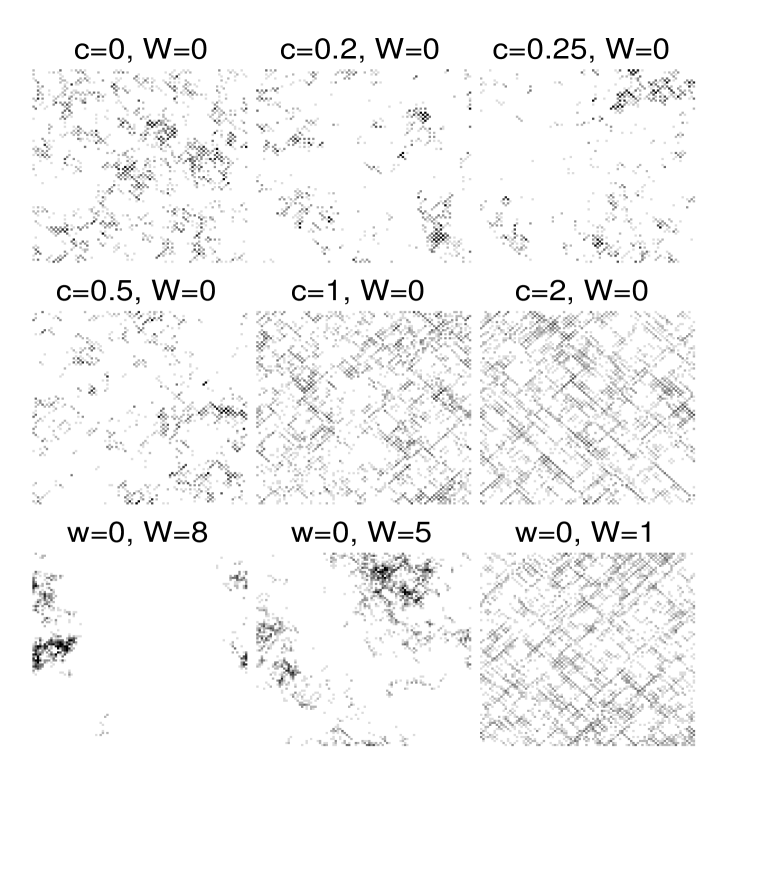
FIG. 1.: Probability density $|\phi_{j}|^{2}$ of the eigenstate $j$ closest to the band center for various off-diagonal and diagonal disorders and system size $L=96$. Different gray levels ($i=0,1,\ldots,6$) distinguish whether $|\phi_{j}(n,m)|^{2}>2^{i}/L^{2}$.

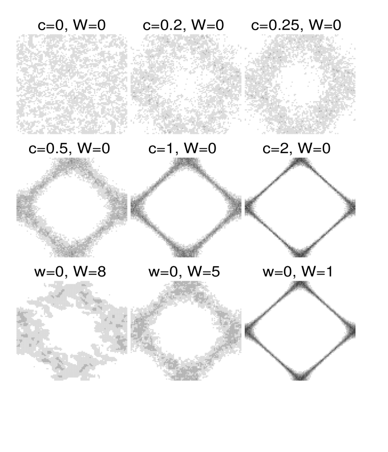
FIG. 2.: Probability density of the Fourier transforms of eigenfunctions with the same parameters as shown in Fig. 1, but averaged over $10$ states close to the band center. Different gray levels ($i=0,1,\ldots,6$) distinguish whether $|\phi_{j}(k_{n},k_{m})|^{2}>2^{i}/L^{2}$.

FIG. 3.: Scaled density of states for purely off-diagonal disorder (thick lines, $W=0$) and, for comparison, purely diagonal disorder (thin lines, $w=0$).

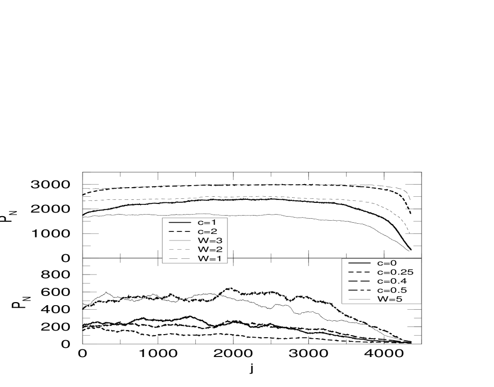
FIG. 4.: Averaged participation numbers $P_{N}$ versus the number $j$ of the eigenstate ordered with increasing energy ($0\leq E_{j}\leq E_{j+1}$) and $N=96\times 96$. Purely off-diagonal disorders are shown by thick lines, purely diagonal disorders by thin lines.

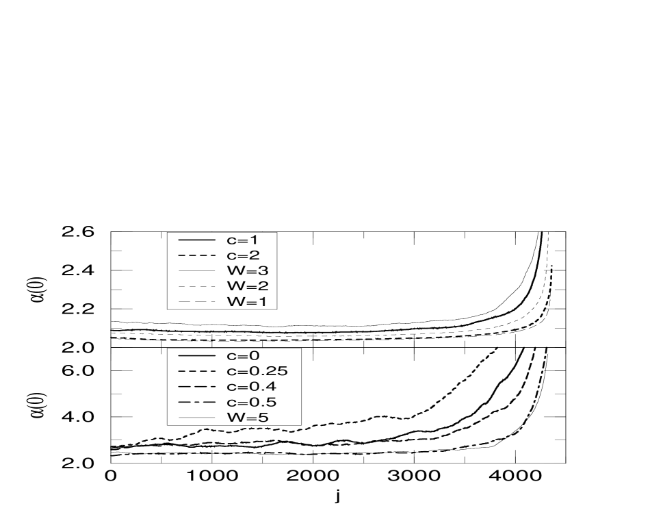
FIG. 5.: Singularity strength $\alpha(0)$ versus the number $j$ of the eigenstate ordered with increasing energy ($0\leq E_{j}\leq E_{j+1}$) and $N=96\times 96$. Purely off-diagonal disorders are shown by thick lines, purely diagonal disorders by thin lines.

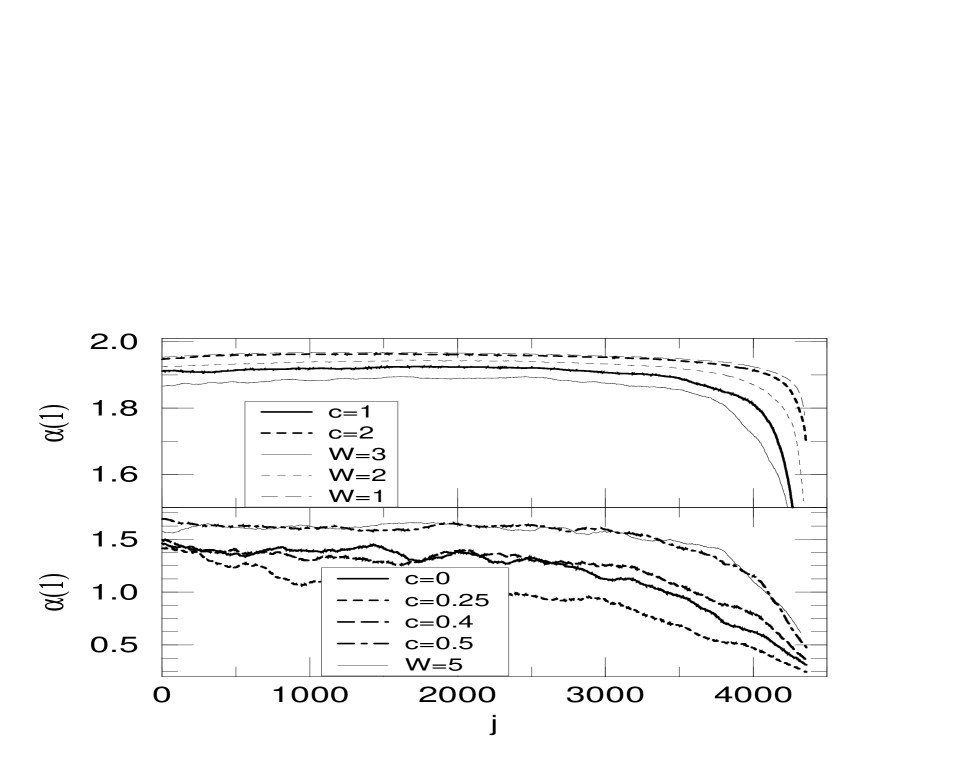
FIG. 6.: Singularity strength $\alpha(1)$ versus the number $j$ of the eigenstate ordered with increasing energy ($0\leq E_{j}\leq E_{j+1}$) and $N=96\times 96$. Purely off-diagonal disorders are shown by thick lines, purely diagonal disorders by thin lines.

FIG. 7.: Finite-size dependence of the participation numbers $P_{N}$ for eigenstates with $c=0$ at energies in the band center ($E=0$), outside the band center but still close to the peak in the DOS ($E=0.1$), and close to the band edge ($E=1.05$).

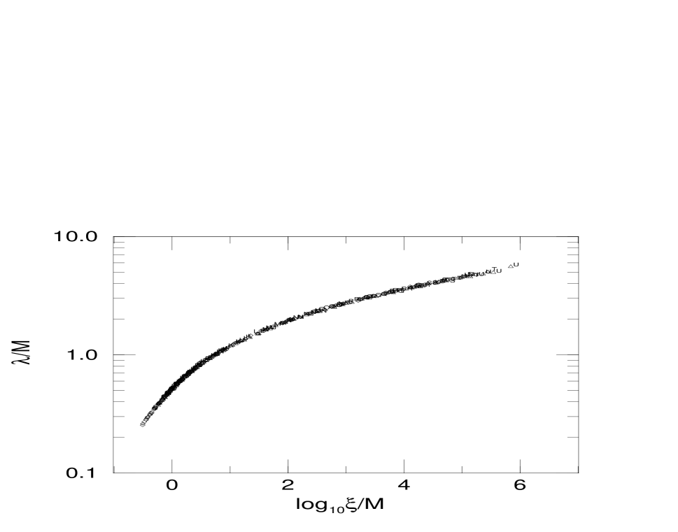
FIG. 8.: Finite-size scaling plot of the reduced localization lengths $\lambda(M)/M$ for purely random hopping ($W=0$) outside the band center with energies $E=0.005$ (characters), $E=0.01$ ($\triangle$) and $E=0.1$ ($\Diamond$). The off-diagonal disorder strengths corresponding to $c=0,0.05,\ldots,1$ are indicated by A, B, $\ldots$, U, respectively.

FIG. 9.: Scaling parameter $\xi$ as a function of off-diagonal disorder center $c$ for $W=0$ and $E=0.005$ (characters), $0.01$ ($\triangle$) and $0.1$ ($\Diamond$).

FIG. 10.: Reduced localization lengths $\lambda(M)/M$ vs. $1/M$ for purely random hopping ($W=0$) and $E=0$. The characters represent different $c$ values as in Figs. 8 and 9. The $\lambda/M$ scale is the same as in Fig. 8 for easier comparison. All curves are parallel to the $1/M$-axis even up to $M=180$ for $c=0.25$ (F).

FIG. 11.: Finite-size scaling plot of the reduced localization lengths $\lambda(M)/M$ for random hopping at $E=0$ and additional potential disorder $W=0.0001$ ($\diamond$), $0.001$ (characters as in Fig. 8), $0.01$ ($\circ$) and $0.1$ ($\Box$). For $W=0.0001$, only data with $M\geq 40$ has been used. The small deviations from FSS at $\xi/M\approx 10$, $\lambda/M\approx 1$ are coming from data for $W=0.001$ and $M=10$.

FIG. 12.: Scaling parameter $\xi$ as a function of off-diagonal disorder center $c$ at $E=0.0$ and diagonal disorder $W=0.0001$ ($\diamond$), $0.001$ (characters), $0.01$ ($\circ$) and $0.1$ ($\Box$).

FIG. 13.: Reduced localization lengths $\lambda(M)/M$ vs. $1/M$ at $E=0$ for random hopping and an additional small potential disorder $W=0.0001$. The $\lambda/M$ scale is the same as in Fig. 11 for easier comparison. The line connects data corresponding to $c=0.25$.

- [1] P. W. Anderson, Phys. Rev. 109, 1492 (1958).
- [2] E. Abrahams, P. W. Anderson, D. C. Licciardello, and T. V. Ramakrishnan, Phys. Rev. Lett. 42, 673 (1979).
- [3] P. A. Lee and T. V. Ramakrishnan, Rev. Mod. Phys. 57, 287 (1985).
- [4] B. Kramer and A. MacKinnon, Rep. Prog. Phys. 56, 1469 (1993).
- [5] F. Wegener, Nucl. Phys. B316, 663 (1989).
- [6] J.-L. Pichard, G. Sarma, J. Phys. C 14, L217 (1981).
- [7] A. MacKinnon and B. Kramer, Z. Phys. B 53, 1 (1983).
- [8] K. Müller, B. Mehlig, F. Milde, and M. Schreiber, Phys. Rev. Lett. 78, 215 (1997).
- [9] D. Belitz and T. R. Kirkpatrick, Rev. Mod. Phys. 66, 261 (1994).
- [10] T. Giamarchi and H. J. Schulz, Phys. Rev. B 37, 325 (1988); T. Giamarchi and B. S. Shastry, Phys. Rev. B 51, 10915 (1995).
- [11] S. V. Kravchenko, D. Dimonian, and M. P. Sarachik, Phys. Rev. Lett. 77, 4938 (1996).
- [12] V. Dobrosavljević, E. Abrahams, E. Miranda, and S. Chakravarty, preprint (1997, cond-mat/9704091).
- [13] D. Belitz and T. R. Kirkpatrick, preprint (1997, cond-mat/9705023).
- [14] M. Schreiber, Phys. Rev. B 31, 6146 (1985); —, J. Phys. C 18, 2493 (1985).
- [15] B. Mandelbrot, The Fractal Geometry of Nature (W. H. Freeman, New York, 1982); J. Feder, Fractals (Plenum, New York, 1988).
- [16] M. Schreiber and H. Grussbach, Phys. Rev. Lett. 67, 607 (1991). M. Schreiber and H. Grussbach, Fractals 1, 1037 (1993); H. Grussbach and M. Schreiber, Phys. Rev. B 51, 663 (1995). F. Milde, R. A. Römer, and M. Schreiber, Phys. Rev. B 55, 9463 (1997).
- [17] N. Dupuis and G. Montambaux, Phys. Rev. B 43, 14390 (1991); B. D. Simons and B. L. Altshuler, Phys. Rev. B 48, 5422 (1993); E. Hofstetter and M. Schreiber, Phys. Rev. B 49, 14726 (1994);
- [18] D. C. Licciardello and D. J. Thouless, J. Phys. C 8, 4157 (1975); — and —, — 11, 925 (1978); D. Weaire and V. Srivastava, J. Phys. C 12, 4309 (1977); J. Stein and U. Krey, Z. Phys. B 37, 13 (1980); — and —, Physica A 106, 326 (1981).
- [19] D. K. K. Lee and J. T. Chalker, Phys. Rev. Lett. 72, 1510, (1994); T. Kawarabayashi, Phys. Rev. B 51, 10897 (1995); D. N. Sheng and Z. Y. Weng, Phys. Rev. Lett. 75, 2388, (1995);
- [20] M. Batsch, doctoral thesis, Universität Hamburg, 1997.
- [21] J. K. Cullum and R. A. Willoughby, Lanczos Algorithms for Large Symmetric Eigenvalue Computations (Birkhäuser, Basel, 1985).
- [22] H. G. E. Hentschel and I. Procaccia, Physica D 8, 435 (1983); A. B. Chabra and R. V. Jensen, Phys. Rev. Lett. 62, 1237 (1989).
- [23] F. Wegener, in Localization and Metal-Insulator Transitions, H. Fritzsche and D. Adler (eds.) (Plenum, New York, 1985) p. 337.
- [24] H. Grussbach, doctoral thesis, Universität Mainz, 1995.
- [25] V. I. Oseledec, Trans. Moscow Math. Soc. 19, 197 (1968).