Two interacting particles in a disordered chain I :
Multifractality of the interaction matrix elements

Abstract

For $N$ interacting particles in a one dimensional random potential, we study the structure of the corresponding network in Hilbert space. The states without interaction play the role of the “sites”. The hopping terms are induced by the interaction. When the one body states are localized, we numerically find that the set of directly connected “sites” is multifractal. For the case of two interacting particles, the fractal dimension associated to the second moment of the hopping term is shown to characterize the Golden rule decay of the non interacting states and the enhancement factor of the localization length.

The wave functions of one particle in a random potential have been extensively studied. In two dimensions within the localization domains fe the large fluctuations of their amplitudes have a multifractal character. In one dimension, the elastic mean free path $l$ and the localization length $L_{1}$ coincide, preventing a single one particle wave function to be multifractal over a significant range of scales. The description of the correlations existing between the localized eigenstates is more difficult. This is quite unfortunate, since a local two-body interaction re-organizes the non interacting electron gas in a way which depends on the spatial overlap of (four) different one particle states. When one writes the $N$-body Hamiltonian in the basis built out from the one particle states (eigenbasis without interaction), this overlap determines the interaction matrix elements, i.e. the hopping terms of the corresponding network in Hilbert space. In this work, we numerically study the distribution of the hopping terms in one dimension, when the one body states are localized. It has been observed fmpw that this distribution is broad and non Gaussian. We give here numerical evidence that this distribution is multifractal. Moreover, since the obtained Rényi dimensions do not depend on $L_{1}$, simple power laws describe how the moments scale with the characteristic length $L_{1}$ of the one body problem. Since the main applications we consider (Golden rule decay of the non interacting states, enhancement factor of the localization length for two interacting particles) depend on the square of the hopping terms, we are mainly interested by the scaling of the second moment. For a size $L\approx L_{1}$, we show that, contrary to previous assumptions, the $N$-body eigenstates without interaction directly coupled by the square of the hopping terms have not a density of the order of the two-body density $\rho_{2}(L_{1})\propto L_{1}^{2}$, but a smaller density $\rho_{2}^{\rm eff}(L_{1})\propto L_{1}^{f(\alpha(q=2))}$. The dimension $f(\alpha(q=2))$ ($\approx 1.75$ for hopping terms involving four different one body states) characterizes the fractal set of $N$-body eigenstates without interaction which are directly coupled by the square of the hopping terms.

We consider $N$ electrons described by an Hamiltonian including the kinetic energy and a random potential, plus a two-body interaction:

$$H=\sum_{\alpha\sigma}\epsilon_{\alpha}d^{+}_{\alpha\sigma}d_{\alpha\sigma}+U\sum_{\alpha\beta\gamma\delta}Q_{\alpha\beta}^{\gamma\delta}d^{+}_{\alpha\downarrow}d_{\gamma\downarrow}d^{+}_{\beta\uparrow}d_{\delta\uparrow}$$ (1)

The operators $d^{+}_{\alpha\sigma}$ ($d_{\alpha\sigma}$) create (destroy) an electron in a one body eigenstate $|\alpha>$ of spin $\sigma$. Noting $\Psi_{\alpha}(n)$ the amplitude on site $n$ of the state $|\alpha>$ with energy $\epsilon_{\alpha}$, the interaction matrix elements are proportional to the $Q_{\alpha\beta}^{\gamma\delta}$ given by:

$$Q_{\alpha\beta}^{\gamma\delta}=\sum_{n}\Psi^{*}_{\alpha}(n)\Psi^{*}_{\beta}(n)\Psi_{\gamma}(n)\Psi_{\delta}(n)$$ (2)

This comes from the assumption that the interaction $U\sum_{n}c^{+}_{n\downarrow}c_{n\downarrow}c^{+}_{n\uparrow}c_{n\uparrow}$ is local. The $c^{+}_{n\uparrow}$ ($c_{n\sigma}$) create (destroy) an electron on the site $n$ and $d^{+}_{\alpha\sigma}=\sum_{n}\Psi_{\alpha}(n)c^{+}_{n\sigma}$. When $U=0$, the Hamiltonian is diagonal in the basis built out from the one particle states, and the $N$ body states ($\prod_{i=1}^{N}d^{+}_{\alpha_{i}\sigma_{i}}|0>$) can be thought as the “sites” with energy $\sum_{i=1}^{N}\epsilon_{\alpha_{i}}$ of a certain network which is not defined in the real space, but in the $N$-body Hilbert space. When $U\neq 0$, different “sites” can be directly connected by off-diagonal interaction matrix elements. Therefore, one can map agkl this complex $N$-body problem onto an Anderson localization problem defined on a particular network in the $N$-body Hilbert space. Since the interaction is two body, only the “sites” differing by two quantum numbers can be directly coupled. This restriction will not matter sh for $N=2$ and (under certain approximations) may yield a Cayley tree topology agkl for the resulting network, if $N$ is large. We study the additional restrictions coming from one body dynamics.

We summarize a few evaluations of the second moment ($q=2$) of $Q_{\alpha\beta}^{\gamma\delta}$ which have been previously used. Case (i): The one body Hamiltonian is described by random matrix theory (RMT). The statistical invariance under orthogonal transformations $O(M)$ implies that $\langle(Q_{\alpha\beta}^{\gamma\delta})^{2}\rangle\approx 1/M^{3}$ where $M$ is the number of one body states. Case (ii): The system is a disordered conductor of conductance $g$. An estimate agkl based on perturbation theory gives $\langle(UQ_{\alpha\beta}^{\gamma\delta})^{2}\rangle\propto(\Delta/g)^{2}$. Since the one particle mean level spacing $\Delta\propto 1/M$, this perturbative result coincides with the previous RMT results if one takes $M\equiv g^{2}$. Moreover, it is valid only if all the one particle states appearing in Eq.(2) are taken from a sequence of $g$ consecutive levels in energy. Otherwise, $Q_{\alpha\beta}^{\gamma\delta}$ can be neglected. Case (iii): The system is a disordered insulator. Shepelyansky sh in his first study of the two interacting particles (TIP), assumes a RMT behavior for the $M=L_{1}^{d}$ components of the wave function inside the localization domain, and neglects the exponentially small components outside this domain. When the dimension $d=1$, one gets a term $(Q_{\alpha\beta}^{\gamma\delta})^{2}\approx 1/L_{1}^{3}$ for the terms coupling a TIP state $|\alpha\beta>$ to $L_{1}^{2}$ TIP states $|\gamma\delta>$. This estimate for $g<1$ differs from the one valid when $g>1$ under two important aspects: not only $M\approx L_{1}^{d}$ instead of $g^{2}$, but the condition for a large hopping is entirely different. In the insulator, a large hopping term is not given by four one particle states close in energy, but by four states close in real space, i.e. located inside the same localization domain. Ponomarev and Silvestrov have criticized ps this estimate, using an approximate description of a localized state for weak disorder. They note that the density of TIP states coupled by the interaction is sensibly smaller.

For a more accurate study of $Q_{\alpha\beta}^{\gamma\delta}$ in one dimension, we consider a spin independent one particle Anderson tight binding model with $L$ sites and nearest neighbor hopping ($t\equiv 1$). The on-site potentials $V_{n}$ are taken at random in the interval [-W,W] and the boundary conditions are periodic. $L_{1}$ is estimated from the weak disorder formula $L_{1}\approx 25/W^{2}$ . The $|Q_{\alpha\beta}^{\gamma\delta}|$ are calculated using Eq.(2) and numerical diagonalization of the one particle Hamiltonian. $Q_{\alpha\beta}^{\gamma\delta}$, for fixed $\alpha$ and $\beta$ is a two-dimensional object which is not defined in the real $2d$ space, but in the space of two one particle quantum numbers $\gamma$ and $\delta$. Those states $|\gamma>$ (and $|\delta>$) can be ordered in different ways: (a) spectral ordering by increasing eigenenergy, (b) spatial ordering by the location $n_{\gamma}$ of their maximum amplitude, from one side of the sample to the other, (c) momentum ordering if $W=0$. Let us note that ordering (b) becomes meaningful only in the localized regime ($L>L_{1}$).

We first study the matrix element $Q_{\alpha_{0}\alpha_{0}}^{\gamma\delta}$, characterizing two electrons with opposite spins in the same state $|\alpha_{0}>$ hopping to an arbitrary state $|\gamma\delta>$. Hopping is very unlikely over scales larger than $L_{1}$. The $L_{1}^{2}$ large values of the hopping term are concentrated inside a square of size $L_{1}^{2}$, as shown in Fig.1 for a given sample using ordering (b) and a rainbow color code. Fig.1 is not homogeneously colored, but exhibits a complex pattern which reminds us another bi-dimensional object: the one particle wave function in a two dimensional disordered lattice. This suggests us to analyze its fluctuations as for the $2d$ one body states, and to check if this pattern is not the signature of a multifractal structure.

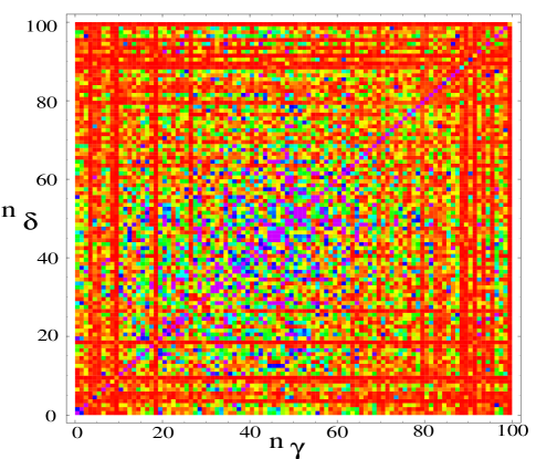
Figure 1: $|Q_{\alpha_{0}\alpha_{0}}^{\gamma\delta}|$ with $|\alpha_{0}>$ taken in the bulk ($n_{\alpha_{0}}=50$) of a sample of size $L=L_{1}=100$. Spatial ordering (b). The color code goes from red (small value) to violet (large value) through yellow, green and blue.

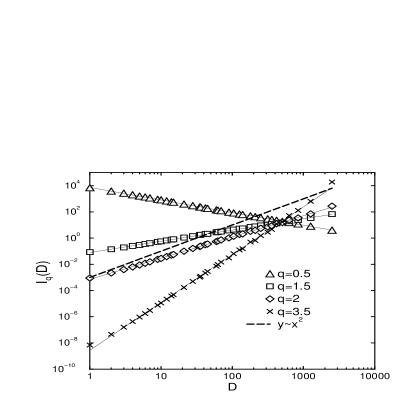
Figure 2: Power laws showing that Fig. 1 corresponds to a multifractal measure in the $(\gamma,\delta)$ two dimensional plane. $I_{q}(D)$ are calculated for a single sample with $L_{1}=L=2500$. $\alpha_{0}$ in the bulk of the spectrum. The states $|\gamma\rangle$ and $\delta\rangle$ are ordered by increasing eigenergy (ordering a). The dashed line corresponds to the RMT prediction (case (i)).

In analogy with the $2d$ one body problem, we do not expect that this multifractality will be valid in the whole $(\gamma,\delta)$ Hilbert space, but only in a limited but parametrically large domain.

We proceed as usual (see references pv ; hjkps ) for the multifractal analysis. For $L_{1}$ and $L$ fixed, we divide the plane $(\gamma,\delta)$ into $(L/D)^{2}$ boxes of size $D$ and we calculate the ensemble averaged function for different values of $q$

$$I_{q}(D)=\sum_{i=1}^{N_{boxes}}\left(\sum_{\gamma,\delta\in\mbox{box}_{i}}|Q_{\alpha_{0}\alpha_{0}}^{\gamma\delta}|\right)^{q}.$$ (3)

The existence of a multifractal measure defined in the $(\gamma,\delta)$-plane by the interaction matrix elements is established in the next figures. In Fig.2, a single sample has been used and power laws $I_{q}(D)\propto D^{\tau(q)}$ are obtained over many orders of magnitude for different values of q.

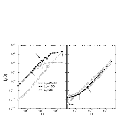
Figure 3: Left: Spatial ordering (b). $I_{2}(D)$ for $|Q_{\alpha_{0}\alpha_{0}}^{\gamma\delta}|$ with $\alpha_{0}$ in the bulk of the spectrum and for $L_{1}$ (indicated by the arrows) $=25,200,2500\leq L=2500$. The power law behaviors are obtained for a given sample if $1\leq D\leq L_{1}$. Right: Same samples using spectral ordering (a). The arrows indicates the lower scales associated to $\Delta(L_{1})$. The power laws are valid for $L/L_{1}\leq D\leq L$.

The limits of validity of these power laws are shown in Fig. 3.

On the left side, spatial ordering (b) for different values of $L_{1}$ is used for the states ($\gamma,\delta$). One can see that $I_{q}(D)\propto D^{\tau(q)}$, for scales $1<D<L_{1}$, as indicated by the arrows. The lower scale is given by the lattice spacing of the $(n_{\gamma},n_{\delta})$ network in Hilbert space. The upper scale $L_{1}$ is the largest scale compatible with a spatial overlap of the states $\gamma$ and $\delta$, for a fixed $\alpha_{0}$. This means that the multifractality of the interaction matrix elements $Q_{\alpha_{0}\alpha_{0}}^{\gamma\delta}$ in the two dimensional Hilbert space $(\gamma,\delta)$ has the same parametrically large range of validity as the one body wave function fe in two dimensions (scale $1<D<L_{1}$). Here, multifractality is valid for $L_{1}^{2}$ matrix elements as multifractality is valid in the $2d$ one body problem for $L_{1}^{2}$ sites.

On the right side of Fig. 3 spectral ordering (a) is used for the same samples, giving the same power laws as with ordering (b), inside the corresponding energy range ($\Delta(L_{1})<D\Delta(L)<1$) indicated by the arrows. $\Delta(x)\propto x^{-1}$ is the level spacing of a segment of size $x$, and 1 is the band width. The exponents $\tau(q)$ are independent of the ordering when $L>L_{1}$ (i.e. when the ordering (b) becomes meaningful) and the small fluctuations from sample to sample are removed by ensemble averaging.

The corresponding Rényi dimensions

$$d(q)\equiv\tau(q)/(q-1)$$

are shown in Fig. 4 for different $L$ and $L_{1}$, using ordering (a) and ensemble averaging.

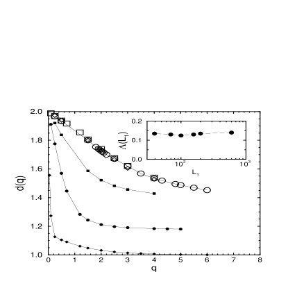
Figure 4: $d(q)$ with $\alpha_{0}$ in the bulk of the spectrum using ordering (a) and after ensemble averaging. Filled symbols: $L=240$ and $L_{1}=\infty$ (diamonds), $25.10^{4}$ (circles) and $2500$ (squares). Open symbols: $L_{1}=70$ and $L=960$ (diamonds), $480$ (circles) and $240$ (squares). Insert: the slope $\Lambda(L_{1})$ showing that $d(q)$ is disorder independent for $q\leq 3$ and $L_{1}<L$.

For an infinite $L_{1}$ (no disorder), the eigenstates are plane waves of momentum $k_{\alpha}$ and $Q_{\alpha\beta}^{\gamma\delta}\neq 0$ only if $k_{\alpha}+k_{\beta}-k_{\gamma}-k_{\delta}=0$. This gives $d(0)=2$ and $d(q>0)=1$ with ordering (c). The dimensions calculated with ordering (a) are close to this limit. For a finite $L_{1}$, $d(q)$ goes from the clean limit ($L<<L_{1}$) to an $L_{1}$-independent regime when $L>>L_{1}$. In the crossover regime ($L\leq L_{1}$) the $d(q)$ depend on $L_{1}$. In the limit $L>>L_{1}$, the $d(q)$ (using orderings (a) or (b)) do not depend on $L$ and $L_{1}$. For $0<q\leq 3$,

$$d(q)\approx 2-\Lambda q$$

with a slope $\Lambda\approx 0.135$. The $L_{1}$-independence of $\Lambda$ is shown in the insert of Fig. 4 for $L_{1}\leq L$ up to $L_{1}=600$.

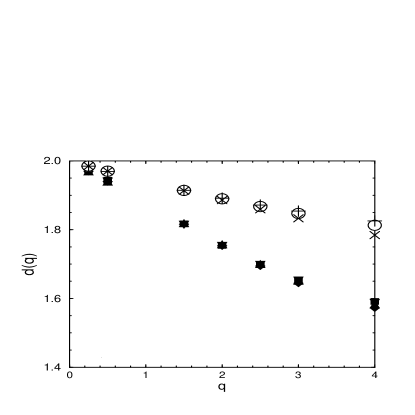
Figure 5: d(q) calculated for $L_{1}=70$ and $L=240$ using ordering (a). The filled symbols correspond to $\alpha=\beta=\alpha_{0}$, averaged over 10 consecutive $\alpha_{0}$ chosen in various parts of the spectrum: down triangle ($130\leq\alpha_{0}\leq 140$), square ($120\leq\alpha_{0}\leq 130$), diamond ($145\leq\alpha_{0}\leq 155$) and up triangle ($170\leq\alpha_{0}\leq 180$). Empty symbols correspond to the case $\alpha\neq\beta$. $\alpha$ is fixed and $d(q)$ is averaged for a few $\beta\neq\alpha$: circle ($\alpha=100,123\leq\beta\leq 133$), cross ($\alpha=80,123\leq\beta\leq 133$) and plus ($101\leq\alpha\leq 112$ and $123\leq\beta\leq 133$)

A multifractal distribution has scaling behavior described by the $f(\alpha)$-spectrum, given by the relations:

$${}\alpha(q)=\frac{d\tau}{dq}{\rm\ \ and\ \ }f(\alpha(q))=\alpha(q).q-\tau(q).$$ (4)

We obtain

$$f(\alpha(q))\approx 2-\Lambda q^{2}$$ (5)

for $q\leq 3$, i.e. a parabolic shape $f(\alpha)=2-(\alpha-2-\Lambda)^{2}/(4\Lambda)$ around the maximum $2+\Lambda$. We have mainly studied the first positive moments, since we are mainly interested by $f(\alpha(q=2))$. Indeed, when one uses Fermi golden rule to calculate the interaction-induced decay of a non-interacting state, one needs to know the density of states directly coupled by the second moment $(q=2)$ of the hopping term. The fractal dimension of the support of this density is given by $f(\alpha(q=2))$. For greater values of $q$, there are deviations around the parabolic approximation, indicating deviations around simple lognormal distributions. From a study of the large and small values of $|Q_{\alpha_{0}\alpha_{0}}^{\gamma\delta}|$, one can obtain $d(q\rightarrow\pm\infty)$. We find $d(+\infty)=1.33$ and $d(-\infty)=3.15$, giving the limits of the support of $f(\alpha)$.

We have also checked that our results for $Q_{\alpha_{0}\alpha_{0}}^{\gamma\delta}$ do not depend on the chosen $\alpha_{0}$ and studied the general case where $|\alpha>$ and $|\beta>$ are not the same. In Fig. 5, one can see that the $Q_{\alpha_{0}\alpha_{0}}^{\gamma\delta}$ studied for different $\alpha_{0}$ give the same curves $d(q)$. Using energy ordering (a) and imposing an energy separation $|\epsilon_{\alpha}-\epsilon_{\beta}|>\Delta(L_{1})$ in order to have a good overlap between the fixed states $\alpha$ and $\beta$, we find also power law behaviors for $I_{q}(D)$. The corresponding dimensions $d(q)$ are given in Fig. 5, characterized by a slope

$$\Lambda(\alpha\neq\beta)\approx\Lambda(\alpha=\beta)/2\approx 0.065.$$

Therefore, the multifractal character of $Q_{\alpha\beta}^{\gamma\delta}$ is less pronounced when $|\alpha>\neq|\beta>$, but remains relevant.

So far, we have discussed the hopping terms of the general $N$-body problem. We now discuss how our results modify previous assumptions for two interacting particles (TIP). As pointed out by Shepelyansky, the interaction induced hopping mixes nearby in energy TIP states $|\alpha\beta>=d^{+}_{\alpha\downarrow}d^{+}_{\beta\uparrow}|0>$. The decay width $\Gamma$ js ; wp ; wpi of a TIP state $|\alpha\beta>$, built out from two one particle states localized within $L_{1}$, can be estimated using Fermi golden rule. If one assumes RMT wave functions inside $L_{1}$ for the one particle states, (case (iii)) the $Q_{\alpha\beta}^{\gamma\delta}\approx\pm U.L_{1}^{-3/2}$ couple the TIP state $|\alpha\beta>$ to all the TIP states $|\gamma\delta>$ inside $L_{1}$. Around the band center, they have a density $\rho_{2}(L_{1})\propto L_{1}^{2}$ and Fermi golden rule gives

$$\Gamma(E\approx 0)\propto\frac{U^{2}}{L_{1}^{3}}\rho_{2}(L_{1})=\frac{U^{2}}{L_{1}}$$ (6)

. We have shown that all the TIP states which can be coupled by the interaction within the localization domains are not equally coupled. Since the square of the hopping terms appears in the Golden rule, our multifractal analysis gives a reduced effective TIP density $\rho_{2}^{\rm eff}\propto L_{1}^{f(\alpha(q=2))}$ which should replace the total TIP density $\rho_{2}(L_{1})$. The resulting expression

$${}\Gamma_{\alpha\beta}\propto\frac{U^{2}}{L_{1}^{3}}L_{1}^{f(\alpha(q=2))}$$ (7)

can be compared to the direct numerical evaluation:

$${}\Gamma_{\alpha\beta}=U^{2}\sum_{\gamma\delta}|Q_{\alpha\beta}^{\gamma\delta}|^{2}\delta(\epsilon_{\alpha}+\epsilon_{\beta}-\epsilon_{\gamma}-\epsilon_{\delta})$$ (8)

of the Golden rule decay.

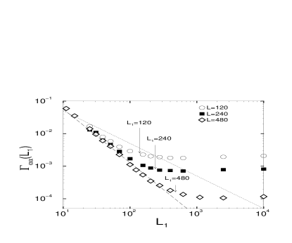
Figure 6: $\Gamma_{\alpha\alpha}(L_{1})$ for three different sizes $L$. Dashed line: $y=2.55L_{1}^{-1.65}$. Doted line: $y=0.5L_{1}^{-1}$

In Fig.6, we show for three different sizes $L$ how the decay rate $\Gamma_{\alpha\alpha}$ numerically calculated using Eq.(8) depends on $L_{1}$, for a TIP state $|\alpha\alpha>$ where $\alpha$ is taken in the bulk of the spectrum. From Fig.4, one gets $\alpha(2)\approx 1.52$ and $\tau(2)\approx 1.69$, and Eq.(4) gives $f(\alpha(q=2))\approx 1.35$. For this value, one can see in Fig.6 that Eq.(7) and Eq.(8) give indeed the same $L_{1}$-dependence. This observed $L_{1}^{-1.65}$ law clearly differs from the $L_{1}^{-1}$ law implied by the RMT assumption (case (iii)). We can also see that $\Gamma_{\alpha\alpha}$ does not depend on $L$ when $L_{1}<L$, since there are no significant hopping terms for range larger than $L_{1}$.

Another interesting issue is the enhancement of the localization length $L_{2}$, which is induced by the interaction and characterizes a restricted set of TIP states which have a sufficient overlap to be re-organized by a local interaction owm ; wmpf . Using the Thouless block scaling analysis i , one finds $\frac{L_{2}}{L_{1}}\propto(\pm U/L_{1}^{3/2}\rho_{2}(L_{1}))^{2}$. If the density $\rho_{2}(L_{1})$ of states coupled by the interaction is the total TIP density for a size $L_{1}$, one finds the original estimate sh ; i $L_{2}\propto L_{1}^{2}$. The multifractality yields a reduced effective density $\rho_{2}^{\rm eff}\propto L_{1}^{f(\alpha(q=2))}$ instead of the total TIP density. Since the contribution of TIP states $|\alpha\beta>$ with $\alpha\neq\beta$ dominates, we use $f(\alpha(2))=1.75$ valid when $\alpha\neq\beta$ and we find $L_{2}\propto L_{1}^{1.5}$. This $L_{1}$-dependence is in agreement with recent numerical results fmpw ; sk . So there is an enhancement, though weaker than the original estimate sh ($L_{2}\propto L_{1}^{2}$), due to the multifractal distribution of the hopping terms.

In summary, we have studied how one particle dynamics (one dimensional localization) can affect the many body problem through non trivial properties of the distribution of the two-body interaction. In a clean system, one has $f(\alpha(2))=1$ and the density of states which are effectively coupled by the interaction is the one particle density $\rho_{1}\propto L$. The disorder, as it is well known, enhances the effect of the interaction, since the effective density $\rho_{2}^{\rm eff}\propto L_{1}^{f(\alpha(2))}$, with $1<f(\alpha(q=2)<2$ for $L=L_{1}$. This enhancement of the density of states coupled by the interaction inside a system of size $\approx L_{1}$ is nevertheless smaller than the one ($\rho_{2}\propto L_{1}^{2}$) given by fully chaotic one body states inside their localization domains. In a second paper wwp , a study of the TIP spectral fluctuations will be presented, showing that statistics is critical (as for the one body spectrum at a mobility edge) if $U$ is large enough, accompanied by multifractal wavefunctions in the TIP eigenbasis for $U=0$. In a third paper dtawp , a study of the dynamics of a TIP wave packet will be presented, showing that the center of mass exhibits anomalous diffusion between $L_{1}$ and $L_{2}$. These three studies provide consistent and complementary observations supporting our claim: multifractality and criticality are relevant concepts for a TIP system with on site interaction in one dimension. Our results go beyond the TIP problem and show that oversimplified two-body random interaction matrix models bf ; fic ; js2 which ignore multifractality in the hopping cannot properly describe the many body quantum motion in Anderson insulators.

We are indebted to S. N. Evangelou for very useful comments.

References

- (1) V.I. Fal’ko and K.B. Efetov, Euro. Phys. Lett. 32, 627 (1995); Phys.Rev.B 52, 17413 (1995).
- (2) K. Frahm, A. Müller-Groeling, J.-L. Pichard and D. Weinmann, Europhys. Lett. 31, 169 (1995).
- (3) B.L. Altshuler, Y. Gefen, A. Kamenev, and L.S. Levitov, Phys. Rev. Lett. 78, 2803 (1997).
- (4) D. L. Shepelyansky, Phys. Rev. Lett. 73, 2067 (1994).
- (5) I.V. Ponomarev and P.G. Silvestrov, Phys. Rev. B 56, 3742 (1997).
- (6) G. Paladin and A. Vulpiani, Phys. Rep 156, 147 (1987).
- (7) T.C. Halsey, M.H. Jensen, L.P. Kadanoff, I. Procaccia and B.I. Shraiman, Phys. Rev A 33, 1141 (1986).
- (8) Ph. Jacquod and D. L. Shepelyansky, Phys. Rev. Lett. 75, 3501 (1995).
- (9) D. Weinmann and J.-L. Pichard, Phys. Rev. Lett. 77, 1556 (1996).
- (10) D. Weinmann, J.-L. Pichard and Y. Imry, J. Phys. 1. France 7 1559 (1997).
- (11) F. von Oppen, T. Wettig and J. Müller, Phys. Rev. Lett. 76, 491 (1996).
- (12) D. Weinmann, A. Müller-Groeling, J.-L. Pichard and K. Frahm, Phys. Rev. Lett. 75, 1598 (1995).
- (13) Y. Imry, Europhys. Lett. 30, 405 (1995).
- (14) P. H. Song and Doochul Kim, cond-mat 9705081 (1997).
- (15) X. Waintal, D. Weinmann and J.-L. Pichard, cond-mat 9801134.
- (16) S. de Toro Arias, X. Waintal and J.-L. Pichard, in preparation.
- (17) O. Bohigas and J. Flores, Phys. Lett. 34B, 261 (1971); 35B, 383 (1971).
- (18) V. V. Flambaum, F. M. Izrailev and G. Casati, Phys. Rev. E54, 2136 (1996).
- (19) Ph. Jacquod and D. L. Shepelyansky, Phys. Rev. Lett. 79, 1837 (1997).