Dissipative Electron Transport through Andreev Interferometers

Abstract

We consider the conductance of an Andreev interferometer, i.e., a hybrid structure where a dissipative current flows through a mesoscopic normal (N) sample in contact with two superconducting (S) “mirrors”. Giant conductance oscillations are predicted if the superconducting phase difference $\phi$ is varied. Conductance maxima appear when $\phi$ is on odd multiple of $\pi$ due to a bunching at the Fermi energy of quasiparticle energy levels formed by Andreev reflections at the N-S boundaries. For a ballistic normal sample the oscillation amplitude is giant and proportional to the number of open transverse modes. We estimate using both analytical and numerical methods how scattering and mode mixing — which tend to lift the level degeneracy at the Fermi energy — effect the giant oscillations. These are shown to survive in a diffusive sample at temperatures much smaller than the Thouless temperature provided there are potential barriers between the sample and the normal electron reservoirs. Our results are in good agreement with previous work on conductance oscillations of diffusive samples, which we propose can be understood in terms of a Feynman path integral description of quasiparticle trajectories.

I Introduction

Recently considerable attention has been devoted to mesoscopic superconductivity, i.e. to the transport properties of mesoscopic systems with mixed normal (N) and superconducting (S) elements, where new quantum interference effects have been discovered. Novel physics appear in such systems because electrons undergo Andreev reflections [1] at the N-S boundaries, whereby the macroscopic phase of a superconducting condensate is imposed on the quasi-particle wavefunctions in the normal regions. If transport in the normally conducting part of the sample is phase coherent, there is a possibility that interference between Andreev scattering at two (or more) N-S interfaces makes the conductance of the hybrid system sensitive to the phase difference $\phi$ between the superconducting elements; in this case one may describe the system as an Andreev interferometer.

This paper is concerned with a theoretical description of hybrid mesoscopic systems of the Andreev interferometer type. In particular we are interested in the normal conductance as a function of the phase difference between the condensates of two separate superconducting elements acting as “mirrors” by reflecting the qausi-particles in the normally conducting element, which in its turn is connected to two electron reservoirs as schematically shown in Fig. 1. The normal electron transport may be in the ballistic regime or in the diffusive regime; both cases will be discussed. In addition we will make the important distinction between the cases when potential barriers or (sharp) geometrical features serve as “beam splitters” at the junctions between the leads and the normal element and when the passage between leads and sample is unhindered by quantum-mechanical scattering between distinct quasi-classical trajectories at these junctions.

FIG. 1.: Schematic picture of an Andreev interferometer consisting of a normal (N) metal (diffusive transport regime) in contact with two superconducting elements (S), which are characterized by the phases $\phi_{1}$ and $\phi_{2}$ of their respective order parameter. The normal metal are in contact with two reservoirs R₁ and R₂ via leads. The thick lines at the junctions between the leads and the normal metal represent potential barriers, which act as beam splitters partially reflecting quasiparticles impinging on the junctions, cf. Fig. 2. If transport is phase coherent quasiparticles at the Fermi level (zero excitation energy) are phase conjugated after Andreev reflection at the N-S interfaces, so that Andreev reflected holes (dashed line) retrace the path of the incoming electrons (full line) and vice versa.

The rest of this introduction will be divided into two parts: (i) a general introduction to the subject of Andreev interferometry and (ii) a qualitative discussion based on quasi-particle trajectories which makes it possible to understand the main features of the conductance oscillations of various types of Andreev interferometers a a function of the superconducting phase difference.

A Origin of conductance oscillations in Andreev interferometers

Already in the early 80’s Spivak and Khmel‘nitskii showed [2] the weak localization corrections to the conductance of a diffusive sample containing two superconducting mirrors to be sensitive to the superconducting phase difference. The effect can be understood in terms of the usual interpretation of weak localization as due to coherent backscattering. The interference of probability amplitudes for classical quasi-particle trajectories (or “Feynman paths”) bouncing off both mirrors will depend on the phases of the respective condensates. Considering a closed diffusive path touching both S-N interfaces — where electrons will be reflected as holes and vice versa — the interference between quasi-particles moving in opposite directions, clockwise and counterclockwise around the path, results in a phase difference of 2$\phi$ between the interfering amplitudes, i.e. twice the phase difference between the two superconductors. This is because the phase picked up due to Andreev reflections off the two mirrors is $\pm\phi$ depending on whether the motion is clockwise or anticlockwise. It follows that the weak localization correction to the conductance of a normal sample with two superconducting mirrors has a component that oscillates with a period equal to $\pi$ as the phase difference between the superconductors is varied.

In the beginning of the 90’s, a dependence on the phase difference $\phi$ was discovered not only for the conductance fluctuations but for the main conductance as well. Not only conductance fluctuations but the ensemble-averaged conductance itself can therefore be controlled by the phase difference between two superconducting mirrors. [3, 4, 5, 6, 7] Hybrid S-N systems (Andreev interferometers) which show such a behaviour at very low temperatures have lead-sample junctions which act as “beam splitters” in the sense that a quasi-particle approaching the junction along a quasi-classical trajectory is only partially transmitted. Hence, a beam splitting junction has the effect of partly reflecting a quasi-particle coming from one N-S interface towards the second N-S interface, as illustrated in Fig. 1. This has the important consequence that when a quasi-particle finally leaves the sample to contribute to the current there is a certain probability for it to have interacted with both superconducting mirrors. To be specific, an electron entering the sample from one reservoir, $R_{1}$ say (referring to Fig. 1), may follow a trajectory (full line) where first it is reflected as a hole by one mirror, say $S_{\phi_{1}}$, then it returns (dashed line in Fig. 1) to bounce off the same junction through which it entered, gets reflected towards the second superconducting mirror $S_{\phi_{2}}$ where it is Andreev reflected as an electron, and finally it passes (full line) through the junction to the second reservoir $R_{2}$ now carrying information about the difference $\phi=\phi_{1}-\phi_{2}$ between the phases of the two superconducting mirrors (the difference appears because the phase picked up on Andreev reflection differs in sign between an electron and a hole). It follows [3, 5] that such trajectories contribute a term to the conductance that oscillates with period 2$\pi$ (rather than $\pi$) as function of $\phi$.

FIG. 2.: A potential barrier at the junction between the normal metal and the lead to a reservoir splits the quasiparticle beam coming from one of the superconducting mirrors (cf. arrows). This makes it possible for quasiparticles having undergone Andreev reflection at both mirrors to contribute to the current even if their excitation energy is zero and therefore reflected hole (electron) excitations retrace the paths of the electron (hole) excitations. It follows that the conductance may depend on $\phi_{1}-\phi_{2}$ even at zero temperature (see text).

As we have indicated above the influence of the superconducting phase difference on the conductance of an Andreev interferometer structure is an interference effect. The macroscopic phases of the superconducting condensates, or — using a different language — of the order parameter or of the gap function of the respective superconducting mirror are imposed on the microscopic wavefunctions of the electron- and holelike quasi-particles when they undergo Andreev scattering at the N-S boundaries. The dominating role of these scattering phases is due to the effect of compensation of the phases gained along the electron- and hole sections of the trajectories connecting the Andreev reflection. Returning to Fig. 1, we note that it illustrates how an electron (hole) with energy infinitely close to but above (below) the Fermi energy follows a trajectory [full (dashed) line] towards an N-S interface. When it gets Andreev reflected as a hole, conservation of energy and momentum makes its energy infinitely close to but below (above) the Fermi energy and the hole (electron) retraces the path [dashed (full) line] of the incoming electron (hole). In this way the phase acquired by an electron is “eaten up” as the hole retraces the electron path in the opposite direction and the net change of phase is due to the Andreev reflection only.

The possibility of phase compensation only exists for quasi-particles whose energies are very close to the Fermi energy. Because energy and momentum is conserved in the Andreev scattering process a quasi-particle with excitation energy $E$ measured from the Fermi energy $\epsilon_{F}$ is reflected as a hole of energy $-E$ and in a direction that differs from the incoming path by an angle of order $E/\epsilon_{F}$. This implies that for finite quasi-particle excitation energies the phase compensation will not be complete. Since the dominating role of the superconducting phase difference is lost when the uncompensated phase along the quasi-particle trajectory connecting the two superconducting mirrors is of order $2\pi$ it follows immediately that only quasi-particles whose excitation energies are less than a critical energy $E_{c}$ may contribute to the $\phi$-dependent part of the conductance. For ballistic samples $E_{c}\sim\hbar v_{F}/L$, while $E_{c}\sim\hbar D/L^{2}$ in the diffusive transport regime, where it is known as the Thouless energy ($v_{F}$ is the Fermi velocity, $D$ is the diffusion constant).

The restriction on quasi-particle excitation energies translates into a temperature dependence, where the Thouless energy sets the characteristic temperature scale. Nazarov et al. [8] and Volkov et al. [9] have for example suggested a “thermal mechanism” that gives a large amplitude of the $2\pi$-periodic conductance oscillations with $\phi$ at temperatures close to the Thouless temperature. Their result is due to a dependence of the effective diffusion coefficient on the energy of the quasiparticles in a hybrid S-N-S sample and will be further discussed below.

In addition to dephasing effects due to finite excitation energies phase coherence may be broken by inelastic scattering. The interference effects described can therefore only be observed if the length $L$ of the normally conducting part of the sample is at most of the order of the phase breaking length $L_{\phi}$ or the normal metal coherence length $L_{T}$, whichever of them is smaller. In the ballistic transport regime $L_{T}=\hbar v_{F}/k_{B}T$, while in the diffusive transport regime one has $L_{T}=\left(\hbar D/k_{B}T\right)^{1/2}$

A large number of experimental and theoretical investigations [8, 9, 10, 11, 12, 13, 14, 15, 16, 17, 18, 19, 20, 21, 22, 23, 24, 25, 26, 27, 28, 29, 30, 31, 32] followed the early work on the tunable conductance of mesoscopic samples of the Andreev interferometer type. For diffusive samples the amplitude of the conductance oscillations has been found to be large in the sense that it is comparable to the conductance in the absence of superconducting elements. The conductance maxima usually appear at even multiples of $\pi$. As discussed by Kadigrobov et al. [18] the situation is quite different for ballistic Andreev interferometers, where the conductance oscillations may be giant — i.e. the oscillation amplitude may be much larger than the conductance in absence of superconducting mirrors. The system discussed in Ref. [18] is shown in Fig. 1; the normal part of a hybrid S-N-S system is weakly coupled to two normal electron reservoirs and hence the dissipative current flows from one reservoir to the other via the normal metal element. Two low-transparency barriers form the junctions between sample and leads (going to the reservoirs) and act as beam splitters in the sense outlined above.

The giant conductance oscillations arises because the structure considered in Ref. [18] permits resonant transmission of electrons and holes via the normal part of the sample. Resonant transmission occurs when the spatial quantization of the electron-hole motion in the mesoscopic normal element leads to allowed energy levels coinciding with the Fermi energy (at zero temperature and small bias voltage the energy of the electrons incident from the source reservoir is equal to the Fermi energy). It follows from the semiclassical Bohr-Sommerfeld quantization rule [cf. Eq. (16) below] that all the $N_{\perp}$ conducting transverse modes in the normally conducting element have one quantized level at the Fermi energy if the phase difference $\phi$ between the two superconductors is equal to an odd multiple of $\pi$. This means that for $\phi=\pi(2k+1),\>k=0,\pm 1,\pm 2...$ each transverse mode can resonantly transmit electrons, and hence $N_{\perp}$ transverse modes contribute to the resonance simultaneously. As a result the amplitude of the conductance oscillations reaches the maximal value $G_{max}=N_{\perp}2e^{2}/h$ when $\phi$ is an odd multiple of $\pi$ (giant oscillations).

B Understanding conductance oscillations in Andreev interferometers in terms of Feynman paths

In all experimental and theoretical studies of Andreev interferometers three types of quasi-particle scattering mechanisms (in various combinations) have to be taken into account. Scattering of charge carriers can be due to:

1. potential barriers or geometrical feautures (beam splitters) at the junctions between the mesoscopic sample and the leads to the electron reservoirs

2. impurity scattering inside the mesoscopic region

3. non-Andreev (normal) reflection from potential barriers at the N-S interfaces.

Here we shall emphasize the crucial role played by beam splitters in distinguishing between different types of oscillation phenomena. Therefore we choose to separately discuss two different types of hybrid S-N-S structures: those with- and those without beam splitters. In particular we will show below that the presence of beam splitters is necessary for conductance oscillations with $\phi$ to appear in the limit of vanishing temperature.

1 Andreev interferometers without beam splitters

In the absence of beam splitters quasiparticles are ballistically injected into the mesoscopic sample along quasi-classical trajectories without suffering any quantum-mechanical scattering between trajectories at the junctions between sample and (leads going to the) reservoirs. In this case the quasi-particles therefore freely pass the contact region without undergoing reflection. It is not difficult to convince oneself that in such a system there are no low energy quasi-particle trajectories connecting the reservoir (or reservoirs) and both superconductors. This is because a quasi-particle with vanishingly small excitation energy is perfectly backscattered at the N-S boundaries in the sense that the angle of Andreev scattering is equal to $\pi$. Therefore such a trajectory can not connect more than two bodies (say, the reservoir and one of the N-S interfaces). Of course, if the energy increases, then due to inelastic Andreev reflection (an electron with energy $E$ is transformed into a hole with energy $-E$; the total energy is conserved since a Cooper pair of zero energy is created) the back-scattering is not perfect and, in contrast to the case when $E=0$, the angle of reflection differs from $\pi$ by a value $\alpha\approx E/\epsilon_{F}$. An interference effect involving the condensate phases of both mirrors is now possible since an electron Andreev-reflected as a hole at the S-N interface follows a different trajectory than the impinging electron and hence has a finite probability not to reach the injector region. In this case, as shown in Fig. 3, it is possible that the trajectory will reach the second superconductor before finally escaping to a reservoir. One may readily evaluate the role of the described inelastic Andreev reflection in the formation of phase sensitive trajectories for both the ballistic and the diffusive case.

FIG. 3.: At finite excitation energies $E$ the path of an Andreev reflected hole (electron) in a ballistic system deviates by a finite angle $\alpha(E)$ from the path of the incoming electron (hole). If $E$ is sufficiently large — but not otherwise — one quasiparticle trajectory may therefore, as shown here, hit both superconductors.

In the ballistic case an injected electron which is Andreev reflected as a hole will not directly return to the injector if the distance $L_{0}$ to the superconducting mirror is large compared to the injector opening $d_{0}$. The precise criterion is that it will not return if $\alpha L_{0}>d_{0}$, where $\alpha\approx E/\epsilon_{F}$ (see Fig. 3). If one takes into account that the excitation energy as explained above is limited by the (ballistic) Thouless energy $E_{c}$ in order for phase coherence to be maintained, one concludes that an interference effect involving both Andreev mirrors is possible only if the injector opening is smaller than the electron deBroglie wavelength; this is because since $\alpha(E)<\alpha(E_{c}=\hbar v_{F}/L_{0})$ it follows that $\alpha L_{0}<d_{0}$ if $d_{0}<\lambda_{B}$. (For a degenerate electron gas the deBroglie wavelength is equal to the Fermi wavelength.) The inevitable conclusion is that an interference mechanism involving thermally excited quasi-particles cannot play a role in realistic experiments using ballistic samples. Under these circumstances the effect of scattering by impurities inside the mesoscopic sample is decisive for the desired interference phenomenon involving two superconducting mirrors to occur. In other words — in the absence of beam splitters — we need to consider a mesoscopic sample in the diffusive transport regime.

In the diffusive case interference between Andreev scattering at two spatially separated superconducting mirrors may occur if the mirror-reflected trajectory diverges from the incident trajectory by more than a de Broglie wavelength, $\lambda_{B}$, which we take to be the width of any particular trajectory. In this case we may say that by inelastic Andreev reflection the reflected quasiparticle is sent into a different, classically distinguishable trajectory. When the separation becomes greater than $\lambda_{B}$ this trajectory interacts with a different set of impurities which will take the reflected particle on a diffusive random walk along a completely different Feynman path. As the distribution of trajectories is homogeneous in the diffusive limit, there is a finite probability for the trajectory (which starts from a reservoir) to include points with Andreev reflections from both superconductors. This implies that the criterion for the incident and reflected trajectories to be sufficiently separated after a diffusing length of $L_{D}$ is $\alpha L_{D}\geq\lambda_{B}$. Since the angle $\alpha\sim E/\epsilon_{F}$ this can be converted to a criterion for the excitation energy of the form $E\geq E_{c}$. We recall that interference is destroyed for energies $E\gg E_{c}$. Hence we conclude that there is a distinct group of quasiparticles with excitation energy around the Thouless energy $\sim E_{c}$ for which there is an interference effect controlled by the superconducting phase difference $\phi$. As a result the temperature dependence of the conductance oscillations is non-monotonic. The amplitude of the oscillations vanishes as the temperature goes to zero and has a maximum when the temperature is of the order of the Thouless temperature $T_{c}=E_{c}/k_{B}$. At elevated temperatures, $T\gg T_{c}$, the parameter controlling the decrease in amplitude of the conductance oscillations is $E_{c}/k_{B}T$. This is simply the relative number of electrons with energy of order $E_{c}$. These electrons are responsible for the interference effect we are discussing, which is nothing but the “thermal effect” of Refs. [8] and [9].

Now we turn to structures with beam splitters; below we show that beam-splitting scattering between different trajectories at the junctions between the mesoscopic sample and the reservoirs qualitatively changes the interference pattern. In this case quasiparticles with low excitation energies, $E<E_{c}$, may contribute — in some cases resonantly — to the interference effects causing the conductance to oscillate as a function the superconducting phase difference.

2 Giant conductance oscillations in Andreev interferometers containing beam splitters

Scattering due to potential barriers or geometrical features at junctions between the mesoscopic region and the reservoirs qualitativly change the nature of quasiparticle trajectories. In particular, a particle reflected from an N-S boundary does not necessarily leave the sample for the reservoir directly. Instead, it may be reflected by the junction and re-enter the mesoscopic region. There is a certain probability that such reflections creates low energy trajectories that connect the reservoir(s) with both superconductors. An example of such a trajectory is shown in Fig. 1.

The role of beam splitters in Andreev interferometers was first payed attention to by Nakano and Takayanagi. [3] A number of other interference phenomena also involving quasi-particles at the Fermi energy (zero temperature phenomena) has been discussed in the literature. For instance, Wees et al. [33] showed that elastic scatterers generate muliple reflections at the N-S boundary resulting in an enhancement of the conductance above its classical value. In ballistic structures resonant tunneling through Andreev energy levels coinciding with the Fermi level was predicted in Refs. [18, 20]. For diffusive structures containing beam splitters a significant increase of the Aharonov-Bohm oscillations of the conductance was shown to exist in Refs.  [13, 14, 19, 20, 21, 22, 24]. Beenakker et al. [15] showed that the angular distribution of quasi-particles Andreev reflected by a disordered normal-metal - superconductor junction has a narrow peak centerd around the angle of incidence. The peak is higher than the coherent backscattering peak in the normal state by a large factor $G/G_{0}$ ($G$ is the conductance of the junction and $G_{0}=2e^{2}/h$). The authors identified the enhanced backscattering as the origin of the increase of the oscillation amplitude predicted in Refs.  [14, 18]. As a final example we note that it was shown in Ref. [21] that the beam splitter violates the “sum rule” according to which the conductance in the absence of junction scattering is equal to the number of transverse modes and does not depend on the superconducting phase difference.

All the mentioned interference phenomena involving quasiparticles at the Fermi level ($E=0$) have the same nature for both ballistic and diffusive structures. This follows from the complete phase conjugation of electron- and hole excitations at the Fermi energy. At the Fermi energy even a random-walk-type of diffusive electron trajectory caused by impurity scattering is completely reversed by the Andreev reflected hole and there is a complete compensation of phase. In particular the giant oscillations of conductance with phase difference $\phi$ is insensitive to impurities, as there is a finite scattering volume in which the phase gains along the electron-hole trajectories are completely compensated.

When the transparency associated with junction scattering has intermediate values both the thermal effect and the resonant oscillation effect contribute simultaneously provided the temperature is close to the Thouless temperature. In experiments measuring the conductance oscillations for structures with beam splitters [4, 10, 11, 12, 16, 26, 27, 28, 29, 30, 34] the temperature was of the order of the Thouless temperature or higher, and hence both effects could contribute. The effects can be distinguished by lowering the temperature below the Thouless temperature, as then the amplitude of the conductance oscillations decrease in the case of the thermal effect (it goes to zero as the temperature goes to zero) while the resonant amplitude of the conductance increases and is maximal at zero temperature. Experimental evidence is just beginning to appear [35, 36, 37]

While the role of the termal mechanism has been investigated in detail in Refs. [8, 9], for the giant conductance oscillations the role of intensity of scattering for all types of scattering mentioned above (normal [non-Andreev] reflection at the N-S boundaries, junction- and impurity scattering) remains without a quantative description. The objective of this paper is to fill this gap.

The paper is organized as follows: in Section II we describe how Andreev interferometers are modelled in this work; in Section III, we develop a resonant perturbation theory to find the conductance in the case of ballistic transport inside the sample and weak coupling of the sample to the reservoirs. In comparison with Ref. [18] we here allow scattering between different conduction channels at the two junctions between sample and leads to reservoirs. In Section IV we in addition take into account the normal reflection that accompanies the Andreev reflection of an electron (hole) at a real normal conductor- superconductor interface, and get an explicit analytical expression for the conductance of the system as a function of the number of transverse channels. For cases when it is inconvenient to get analytical results, such as when the coupling is not weak, we present some results of numerical calculations in Section V. Then, in Section VI we relax the condition of the sample being in the ballistic transport regime and calculate the giant conductance oscillations for a diffusive hybrid S-N-S structure using the Feynman path integral approach for the transition probability amplitude. In the conclusions, Section VII, we discuss the range of parameters for which the conductance oscillations can be giant in real experiments.

II Model for an Andreev interferometer

In this Section we describe our model for an Andreev interferometer. As schematically shown in Fig. ref system it consists of a superconductor-normal (semiconductor)-superconductor (S-N-S) sample coupled to two normal electron reservoirs between which a voltage bias is applied. Appealing to experiments [34, 38, 39, 40, 41] we neglect scattering of electrons by impurities inside the sample for the time being and return to this point in Section VI. Nevertheless, the junctions between the S-N-S sample and the normal leads to the electron reservoirs inevitably are sources of scattering. So, whereas we consider electron transport to be adiabatic inside the sample — the current being carried in $N_{\perp}$ channels (modes) — electrons can be scattered between different conduction channels at these junctions. Taking this into account amounts to a first generalization of our earlier treatment of this problem. [18] In our model the coupling between the sample and the reservoirs is controlled by potential barriers (beam splitters, see above) appearing at the junctions between the leads from the reservoirs and the sample. We assume that in the case of low barrier transparency the approximation of a nearly isolated sample is adequate and that channel mixing is absent; we shall then study what happens when the coupling increases in Section III.

FIG. 4.: Schematic picture of an Andreev interferometer of the same type as shown in Fig. 1. The full [dashed] arrows indicate electrons (e) [holes (h)] moving in the ballistic segments 1-5 of the sample. In the model calculation described in the text Andreev- and/or normal scattering may occur at the two superconducting mirrors (S) and scattering between different segments and channels (modes) may occur at the junctions marked A and B.

Another fact ignored in our earlier work [18] is the possible “normal” reflection of quasiparticles by a Schottky barrier at the S-N boundaries, a mechanism that would compete with the Andreev reflection. When normal reflection is possible the degeneracy of the quasiparticle energy levels (Andreev levels) which occurs at the Fermi level for certain values of the phase difference between the two superconductors is lifted and the “giant” conductance oscillations as a function of this phase difference is greatly reduced. Despite the experimental fact that the probability for normal reflection is small [34, 38, 39, 40, 41] the criteria for how small the normal reflection probability must be for the giant oscillations to survive is obviously an important question, which we consider in Section IV. Below we formulate our transport problem for a general case which includes both the possibility for scattering between conduction channels at the sample-lead junctions and normal reflections at the N-S interfaces.

It is convenient to divide our model Andreev interferometer into five different segments so that the electron transport to a good approximation is adiabatic in each segment. We then use a phenomenological method for describing the two manifestly non-adiabatic junction regions [marked A and B in Fig. ref system]. The quasi-particle wave functions in the adiabatic segments 1-5 shown in Fig. 4 can be found with the help of the Bogoliubov-de-Gennes equation. As channel mixing is absent in the adiabatic segments the electron- and hole like components of the wave function in the $n$:th transverse mode in segment $\alpha$ is

$$u_{\alpha}(x,y)=\sum_{n=1}^{N_{\perp}}\left(a_{\alpha,n}^{(e)}e^{ik_{n}^{(e)}x}+b_{\alpha,n}^{(e)}e^{-ik_{n}^{(e)}x}\right)\sin k_{\perp}(n)y$$ (1)

$$v_{\alpha}(x,y)=\sum_{n=1}^{N_{\perp}}\left(a_{\alpha,n}^{(h)}e_{n}^{-ik^{(h)}x}+b_{\alpha,n}^{(h)}e_{n}^{ik^{(h)}x}\right)\sin k_{\perp}(n)y$$ (2)

Here $a_{\alpha,n}^{(e)}$ and $b_{\alpha,n}^{(e)}$ [$a_{\alpha,n}^{(h)}$ and $b_{\alpha,n}^{(h)}$] are the probability amplitudes for free motion of electrons [holes] forward and backward, respectively, in channel $n$ and segment $\alpha$ of the sample; $k_{\perp}(n)=n\pi/d,n=0,1,2,\ldots$ is the quantized transverse wavevector assuming a hard wall confining potential, $d$ is the width of the sample, $k^{(e,h)}_{n}=[k_{F}^{2}-k_{\perp}^{2}(n)\pm 2mE/\hbar^{2}]^{1/2}$ is the electron (hole) longitudinal momentum, $k_{F}$ is the Fermi wavevector, $E$ is the electron energy measured from the Fermi energy, while $x$ and $y$ are longitudinal and transverse coordinates in the sample, respectively. Non-adiabatic scattering of electrons in the junction regions, see Fig. 4, is described by a unitary scattering matrix $\hat{S}$ connecting the wave functions in the surrounding sample segments. Scattering at these junctions mix the transverse modes (channels) in the adiabatic segments (which here and below, for the sake of simplicity, are considered to have the same number of open transverse channels). Hence, the scattering matrix connects ${\bf c}_{\alpha}^{(in)}$ and ${\bf c}_{\alpha}^{(out)}$, which are $N_{\perp}$ -component vectors whose coefficients $a_{\alpha,n}^{(e,h)}$, $b_{\alpha,n}^{(e,h)}$ describe the incoming and outgoing adiabatic wave functions [see Fig. 5 and Eq. (2)],

$${\bf c}_{\alpha}^{(out)}=\sum_{\beta=1}^{3}{\bf\hat{S}}_{\alpha\beta}{\bf c}_{\beta}^{(in)}$$ (3)

We assume the coupling matrix ${\bf\hat{S}}$ to be symmetric with respect to the left and right sample segments [labeled 2 and 4 in Fig. 4]. Therefore the matrix can be written as

$${\bf\hat{S}}=\left(\begin{array}[]{ccc}{\bf\hat{s}}_{11}&{\bf\hat{s}}_{12}&{\bf\hat{s}}_{12}\\ {\bf\hat{s}}_{12}&{\bf\hat{s}}_{22}&{\bf\hat{s}}_{23}\\ {\bf\hat{s}}_{12}&{\bf\hat{s}}_{23}&{\bf\hat{s}}_{22}\\ \end{array}\right)\;,$$ (4)

where ${\bf\hat{s}}_{\alpha\beta}$ are $N_{\perp}\times N_{\perp}$ matrices which mix the conduction channels when an electron (or hole) is transferred from the $\beta$ - to the $\alpha$ segment. Electrons and holes are, however, not mixed. The elements of ${\bf\hat{s}}_{\alpha\beta}^{nm}$ ($n,m=1,2,...N_{\perp}$) are the probability amplitudes for an electron (or hole) in the $m$-th channel of the $\beta$-section to be transferred to the $n$-th channel of the $\alpha$-section. We assume that scattering of an incident quasiparticle at the junction causes transmission of the electron into each of the $N_{\perp}$ open transverse channels with a probability, which is of the same order of magnitude for all channels. This implies that the matrix elements of the matrices $\hat{s}_{12}$, $\hat{s}_{22}$, $\hat{s}_{23}-1$ and $\hat{s}_{11}-1$ are of order $1/\sqrt{N_{\perp}}$.

FIG. 5.: Detail of the junction (A, B in Fig. 4) coupling the reservoirs via leads to the normal part of the system. A scattering matrix connects the amplitudes of incoming- and outgoing quasiparticles, see text.

We choose to parametrize the ${\bf\hat{S}}$ matrix in a way such that there is no channel mixing if the sample is completely decoupled from the reservoirs. This coupling is determined by the elements of the matrix ${\bf\hat{s}}_{12}$ which are the probability amplitudes for electron (hole) transitions from a lead (segments 1 or 5) to the sample (segments 2, 3 or 3,4). In order to describe the strength of the coupling we introduce the parameter $\epsilon_{r}$ and write

$${\bf\hat{s}}_{12}=\left(\frac{\epsilon_{r}}{N_{\perp}}\right)^{1/2}{\bf\bar{s}}_{12}\;.$$ (5)

The scattering matrix (4) has to be unitary — a requirement that leads to five relations between the eight matrices ${\bf\hat{s}}_{\alpha\beta}$, see Eqs. (88-92) in Appendix A. (Note that each matrix has an independent Hermitian and anti-Hermitian part). We are thus left with three undetermined matrices, which we choose to be ${\bf\hat{s}}_{12}$ and the anti-Hermitian part of ${\bf\hat{s}}_{22}$ (the last choice is made only for the sake of calculational convenience, see Appendix A. We assume the Hermitian and anti-Hermitian parts of ${\bf\hat{s}}_{22}$ to be of the same order in the parameter $\epsilon_{r}$ since in the general case they are connected by a Kramers-Kronig relation. It follows from the unitarity conditions that the matrix elements of ${\bf\hat{s}}_{12}$ are of order $1/\sqrt{N_{\perp}}$. Hence the matrix elements of ${\bf\bar{s}}_{12}$ are of order unity.

The conductance of our model system is in the limit of vanishing bias voltage determined by the Landauer formula as modified by Lambert for a system with Andreev reflections [7]:

$$G=\frac{2e^{2}}{h}\left(T_{0}+T_{A}+\frac{2(R_{A}R_{A}^{\prime}-T_{A}T_{A}^{\prime})}{T_{A}+T_{A}^{\prime}+R_{A}+R_{A}^{\prime}}\right)\;.$$ (6)

Here $e$ is the electron charge, $h$ is Planck’s constant and

$$T_{A}=\sum_{k=1}^{N_{\perp}}\tau_{k}^{(A)}, R_{A}=\sum_{k=1}^{N_{\perp}}\rho_{k}^{(A)}$$ (7)

$$T_{0}=\sum_{k=1}^{N_{\perp}}\tau_{k}^{(0)}, R_{0}=\sum_{k=1}^{N_{\perp}}\rho_{k}^{(0)}.$$ (8)

In Eq. (8) $\tau_{k}^{(0)}$ [$\tau_{k}^{(A)}$] is the probability for an electron approaching the sample in the $k$-th transverse channel of the left lead to be transmitted as an electron (hole) into any of the outgoing channels of the right lead. The quantity $\rho_{k}^{(0)}$ [$\rho_{k}^{(A)}$] is the probability for the same electron to be reflected as an electron (hole) into any outgoing channel in the same left lead it came from. Similarily, $\tau_{k}^{{\prime}(0)}$ [$\tau_{k}^{{\prime}(0)}$] and $\rho_{k}^{{\prime}(0)}$ [$\rho_{k}^{{\prime}(A)}$] are normal (Andreev) probabilities for an incoming electron from the $k$-th transverse channel of the right lead to be transmitted as an electron (hole) into any outgoing channel of the left lead and to be reflected as an electron (hole) back into any outgoing channel of the right lead, respectively.

In order to proceed we have to solve the matching equations for the adiabatic wave functions in sample and leads. The matching problem under consideration is illustrated in Fig. 4 where solid and dashed arrows symbolically show electron- and hole plane waves moving to the right and to the left, respectively. The coefficients ${\bf a}_{\alpha}^{(e,h)}$ and ${\bf b}_{\alpha}^{(e,h)}$ are $N_{\perp}$-component vectors, the components of which are the probability amplitudes $a_{\alpha,n}^{(e,h)}$ and $b_{\alpha,n}^{(e,h)}$, see Eq. (2). Matching the wave functions at the junctions using Eq. (3) one gets the following set of equations for these amplitudes:

$$\left\{\begin{array}[]{l}{\bf b}_{1}^{(e,h)}={\bf\hat{s}}_{11}{\bf a}_{1}^{(e,h)}+{\bf\hat{s}}_{12}{\bf a}_{2}^{(e,h)}+{\bf\hat{s}}_{12}{\bf b}_{3}^{(e,h)};\\ {\bf b}_{5}^{(e,h)}={\bf\hat{s}}_{11}{\bf a}_{5}^{(e,h)}+{\bf\hat{s}}_{12}\hat{U}_{3}^{(e,h)}{\bf a}_{3}^{(e,h)}+{\bf\hat{s}}_{12}\hat{U}_{4}^{(e,h)}{\bf b}_{4}^{(e,h)}\\ \end{array}\right.$$ (9)

and

$$\left\{\begin{array}[]{l}{\bf b}_{2}^{(e,h)}-{\bf\hat{s}}_{22}{\bf a}_{2}^{(e,h)}-{\bf\hat{s}}_{23}{\bf b}_{3}^{(e,h)}={\bf\hat{s}}_{12}{\bf a}_{1}^{(e,h)};\\ {\bf a}_{3}^{(e,h)}-{\bf\hat{s}}_{23}{\bf a}_{2}^{(e,h)}-{\bf\hat{s}}_{22}{\bf b}_{3}^{(e,h)}={\bf\hat{s}}_{12}{\bf a}_{1}^{(e,h)};\\ \hat{U}_{3}^{(e,h){\dagger}}{\bf b}_{3}^{(e,h)}-{\bf\hat{s}}_{22}\hat{U}_{3}^{(e,h)}{\bf a}_{3}^{(e,h)}-{\bf\hat{s}}_{23}\hat{U}_{4}^{(e,h){\dagger}}{\bf b}_{4}^{(e,h)}={\bf\hat{s}}_{12}{\bf a}_{5}^{(e,h)};\\ \hat{U}_{4}^{(e,h){\dagger}}{\bf a}_{4}^{(e,h)}-{\bf\hat{s}}_{23}\hat{U}_{3}^{(e,h)}{\bf a}_{3}^{(e,h)}-{\bf\hat{s}}_{22}\hat{U}_{4}^{(e,h)}{\bf b}_{4}^{(e,h)}={\bf\hat{s}}_{12}{\bf a}_{5}^{(e,h)};\end{array}\right.$$ (10)

Here the diagonal matrices $\hat{U_{\alpha}}^{(e,h)}$ simply keep track of the phase gained by electrons and holes during their free motion across segment $\alpha$. The diagonal matrix elements are

$$\begin{array}[]{ccc}u_{\alpha}^{(e)}(n)=e^{ik^{(e)}_{n}l_{\alpha}},&u^{(h)}_{m}(n)=e^{-ik^{(h)}_{n}l_{\alpha}},&n=1,2,\ldots N_{\perp}\end{array}$$ (11)

where $l_{\alpha}$ is the length of section $\alpha$ in Fig. 4.

The set of equations (9) and (10) must be supplemented with boundary conditions at the N-S interfaces. In the general case when both Andreev- and normal reflections at the N-S boundaries are possible the boundary conditions are

$$a_{2,n}^{(e)} = e^{i\Psi_{1}}\left[r_{N}^{(1)}e^{i2k^{(e)}(n)l_{2}}b_{2,n}^{(e)}+r_{A}^{(1)}e^{i\delta k(n)l_{2}}b_{2,n}^{(h)}\right]$$ (12)

$$a_{2,n}^{(h)} = e^{i\Psi_{1}}\left[-r_{A}^{(1)*}e^{i\delta k(n)l_{2}}b_{2,n}^{(e)}+r_{N}^{(1)*}e^{-i2k^{(h)}(n)l_{2}}b_{2,n}^{(h)}\right]$$ (13)

for the left (first) boundary [$\delta k\equiv k^{(e)}-k^{(h)}$] and

$$b_{4,n}^{(e)} = e^{i\Psi_{2}}\left[r_{N}^{(2)}a_{4,n}^{(e)}+r_{A}^{(2)}a_{4,n}^{(h)}\right]$$ (14)

$$b_{4,n}^{(h)} = e^{i\Psi_{2}}\left[-r_{A}^{(2)*}a_{4,n}^{(e)}+r_{N}^{(2)*}a_{4,n}^{(h)}\right]$$ (15)

for the right (second) boundary, see Fig. 4. The probability amplitudes for normal- and Andreev reflections at the N-S boundary are given by $e^{i\Psi}r_{N}$ and $e^{i\Psi}r_{A}$. It follows that $|r^{(1,2)}_{N}|^{2}+|r^{(1,2)}_{A}|^{2}=1$. [42] For convenience explicit expressions for these quantities in terms of the complex order parameter of the superconductor and the reflection- and transmission probability amplitudes of the normal barrier at the N-S interface are given in Appendix B.

The equations (9), (10), (13), and (15) together with the conductance formula (6) form a complete set of equations that permits us to find the conductance of the system under consideration.

In the next section we discuss the non-adiabatic scattering of electrons at the junctions and present analytical formulae for the case of a weak coupling of the sample to the reservoirs ($\epsilon_{r}\ll 1$) and numerical results of computer simulations in the general case. The role of the non-Andreev (normal) reflection at the N-S boundaries is discussed in section IV.

III Role of scattering and mode mixing at the points of coupling to the reservoirs

We start our analysis by assuming a weak coupling between sample and (leads to) reservoirs. In this case the parameter $\epsilon_{r}$ introduced in Eq. (5) is much smaller than one. It is convenient to develop a qualitative understanding starting from the so called Andreev levels that form in the isolated sample when $\epsilon_{r}$ is strictly zero. We consider values of $\phi$ near odd multiples of $\pi$ for which Andreev levels will appear at the Fermi energy ($\phi=\phi_{2}-\phi_{1}$; $\phi_{1}$ and $\phi_{2}$ are the phases of the gap functions in the left and right superconductor, see Fig. 4). We concentrate on energies in a narrow interval $\Delta E\sim\epsilon_{r}\hbar v_{F}/L$ around the Fermi energy, whithin which the quantum states of electrons perturbed by a coupling of the sample to the reservoirs are expected to be found ($\hbar v_{F}/L$ is the characteristic spacing of mode energy levels near the Fermi energy).

By solving the matching equations (10), (13), and (15) for $\epsilon_{r}=0$, using Eqs. (117), (119), and (120) of Appendix B one recovers the following expression [43] for the low energy spectrum of electron-hole quasiparticles in the normally conducting semiconductor sandwiched between two superconducting mirrors

$$\pi(2l+1)\pm\phi=\left(\sqrt{k_{F}^{2}-k_{\perp}(n)^{2}+2mE/\hbar^{2}}-\right.$$ (16)

$$\quad\quad\left.\sqrt{k_{F}^{2}-k_{\perp}(n)^{2}-2mE/\hbar^{2}}\right)L,\quad l=0,\pm 1,\pm 2,\ldots$$ (17)

Here $m$ is the electron mass, $L=l_{2}+l_{3}+l_{4}$ is the length of the normal part of the sample. and all reflections are assumed to be of the Andreev type. The phase $\phi$ comes with a plus- or a minus sign in Eq. (16) depending on whether the electron-hole excitations move as electrons or holes when going from the left to the right S-N interface.

Expression (16) for the spectrum tells us that when $\phi=\pi(2l^{\prime}+1)$ there is one Andreev state at the Fermi level for each transverse mode (index $n$) simultaneously, i.e., the energy of the state whose quantum number $l$ associated with the longitudinal motion equals $l^{\prime}$ coincides with the Fermi energy irrespective of mode number $n$. Therefore, the degeneracy of the energy level at the Fermi energy ($E=0$) is given by the number of open transverse modes $N_{\perp}$, whenever $\phi$ equals an odd multiple of $\pi$. This results in a giant probability for resonant transmission of electrons from one reservoir to the other. The amplitude of the corresponding conductance oscillations, $\Delta G\propto N_{\perp}e^{2}/\hbar$ [18], is therefore much larger than the conductance quantum.

A finite coupling of the sample to the reservoirs (which is of course necessary for a current to be observable) simultaneously results in a broadening and a shift of the Andreev energy levels. The former effect is due to quasiparticle tunneling from the sample to the reservoirs after a finite time, the latter is due to mixing of the transverse modes that inevitably accompanies a finite coupling. Below we show the broadening and the shift to be of the same order in the transparency of the barrier connecting sample and reservoirs. The result is a broadening of the peaks of resonant sample conductance but their giant amplitude remains. This is beacuse a Breit-Wigner type of resonance is broadened without loss of amplitude when the coupling is increased. It turns out that the broadening of each state tends to compensate the shifting around of the energies of previously degenerate states. Readers who are not interested in technical details may want to turn directly to Eq. (35), which expresses this result. Results of numerical calculations presented in Section V show this picture to hold up to a value for $\epsilon_{r}$ which is about half its maximum value. A further increase of the coupling results in a large decrease of the amplitude and increase of the broadening of the peaks.

In the weak coupling case the set of equations (9), (10), (13), and (15) which determines the transmission probability amplitudes can be solved analytically by perturbation theory in the small parameter $\epsilon_{r}$. Below this perturbation theory will be developed.

As shown in Appendix A, all the matrices which describe scattering of electrons and holes inside the sample ($\hat{s}_{22}$ and $\hat{s}_{23}-\hat{1}$) are proportional to $\epsilon_{r}$ if the coupling matrix $\hat{s}_{12}$ is proportional to $\sqrt{\epsilon_{r}}$ and if $\epsilon_{r}\ll 1$ . Hence it follows that the set of equations (9-15) can be written in the form

$$\left({\bf\hat{W}}(E)-\epsilon_{r}{\bf\hat{\Omega}}\right)|{\bf H}\rangle={\left(\frac{\epsilon_{r}}{N_{\perp}}\right)}^{1/2}|{\bf K}\rangle\;.$$ (18)

The vector $|{\bf H}\rangle$ has $12N_{\perp}$ unknown components, viz. ${\bf a}_{i}^{(e,h)},$ ${\bf b}_{i}^{(e,h)}$ for $i=$2, 3, and 4. The vector $|{\bf K}\rangle$ has $4N_{\perp}$ known elements, ${\bf a}_{k}^{(e,h)}$ for $k=$1 and 5, and $8N_{\perp}$ elements which are zero. The matrix ${\bf\hat{W}}(E)$ has $12N_{\perp}$ block matrices along the diagonal with non-zero elements

$$[{\bf W}_{\alpha,\beta}(E)]_{nm}=\delta_{nm}{\bf w}_{\alpha\beta}^{(n)}(E)\quad,$$ (19)

where $\alpha,\beta=1,2,\ldots 12$; $n,m=1\ldots N_{\perp}$. The matrix ${\bf\hat{w}}^{(n)}(E)$ has been obtained for the $n$-th fixed transverse mode in the absence of coupling ($\epsilon_{r}=0$) by matching the electron- and hole components of the wave functions at the N-S boundaries using Eqs. (13) and (15) and at the junctions coupling the sample to the electron reservoirs using Eq. (10) for fixed channel number $n$ and $\epsilon_{r}=0$. The matrix ${\bf\hat{\Omega}}$ has elements describing mixing between modes. The explicit forms of operators $\hat{\bf W},\hat{\bf\Omega}$ and vectors $|{\bf H}\rangle,|{\bf K}\rangle$ are straightforwardly found by comparing Eqs. (10) and (18).

In order to use the resonant perturbation theory we have to consider some properties of the unperturbed system relevant to our problem. It is straightforward to see from (19) that the determinant of the matrix ${\bf\hat{W}}(E)$ can be written as a product of $N_{\perp}$ factors

$$\mbox{Det}{\bf\hat{W}}(E)=\mbox{Det}{\bf\hat{w}}^{(1)}(E)\times\ldots\times\mbox{Det}{\bf\hat{w}}^{(N_{\perp})}(E)$$ (20)

and that its value iz zero at any eigenvalue $E=E_{n,l}$ of the unperturbed system. The eigenfunctions $|\psi_{l}^{(n)}\rangle$ of the unperturbed problem satisfy the following equation

$${\bf\hat{W}}(E_{n,l})|\psi_{l}^{(n)}\rangle=0$$ (21)

Developing the perturbation theory we assume the following inequality to be satisfied.

$$\lambda_{F}\ll d\ll L\;,$$ (22)

where $\lambda_{F}$ is the de-Broglie wave length (Fermi wave length) of the electron, while $d$ and $L$ is the width and length of the sample. We note that the perturbation of the energy has to be much smaller than the distance between neighbouring energy levels corresponding to quantization of the longitudinal motion of electrons, that is

$$\epsilon_{r}\hbar v_{F}/L\ll\hbar v_{F}/L\;.$$ (23)

Here we develop the perturbation theory for a general case in order to use the results also in the next section. Therefore in order to find the correct zero order wave-function the vector $|{\bf H}\rangle$ must be taken as a superposition of the $N_{R}$ states inside the resonant region ($N_{R}$ is possibly but not necessarily smaller than $N_{\perp}$)

$$|{\bf H}\rangle=\sum_{n=1}^{N_{R}}\gamma_{n}|\psi_{l}^{(n)}\rangle+|{\bf H}_{1}\rangle\;.$$ (24)

The summation in (24) goes over the $N_{R}$ transverse modes inside the resonant region, which extends over an interval of order $\epsilon_{r}\hbar v_{F}/L$ on either side of the Fermi energy; $|{\bf H}_{1}\rangle$ is a small addition $\propto\epsilon_{r}$. The unknown coefficients $\gamma_{n}$ should be found with the solvability condition of the equation for $|{\bf H}_{1}\rangle$ that is readily available from Eq. (18) in the linear approximation in $\epsilon_{r}\ll 1$:

$${\bf\hat{W}}(E)|{\bf H_{1}}\rangle= - \sum_{n=1}^{N_{R}}\gamma_{n}[{\bf\hat{W}}^{\prime}(E_{n,l})(E-E_{n,l})-\epsilon_{r}{\bf\hat{\Omega}}]|\psi_{l}^{(n)}\rangle$$ (25)

$$+ {\left(\frac{\epsilon_{r}}{N_{\perp}}\right)}^{1/2}|{\bf K}\rangle$$ (26)

Here the superscript “prime” indicates derivation with respect to energy $E$. When obtaining Eq. (26) we used the inequality (23) and expanded ${\bf\hat{W}}(E)$ in a Taylor series around $E_{n,l}$ (with the restriction $|E-E_{n,l}|\ll\hbar v_{F}/L$) in every term of the sum and took into account Eq. (21).

Multiplying both sides of Eq. (26) from the left by bra-vectors $\langle\psi_{l}^{(m)}|$ [which can be determined from the equation $\langle\psi_{l}^{(m)}|{\bf\hat{W}}(E_{m})=0$] one readily gets the solvability conditions for Eq. (26) that determines the coefficients $\gamma_{n}$. In this way we obtain the main equation which has to be solved in order to get $\gamma_{n}$; these coefficients, according to Eqs. (9) and (24), determine the probability of the resonant transmission of an electron from one reservoir to the other via the sample):

$$\sum_{n=1}^{N_{R}}\left[i(E-E_{n})W_{n}^{\prime}\delta_{mn}-\epsilon_{r}\Omega_{mn}\right]\gamma_{n}=\left(\frac{\epsilon_{r}}{N_{\perp}}\right)^{1/2}K_{m}\;.$$ (27)

Here we have used the short hand notation

$$W_{n}^{\prime}=-i\langle{\bf\psi}^{(n)}|{\bf\hat{W}}^{\prime}(E_{n})|{\bf\psi}^{(n)}\rangle$$ (28)

$$\Omega_{mn}=\langle{\bf\psi}^{(m)}|{\bf\hat{\Omega}}|{\bf\psi}^{(n)}\rangle$$ (29)

$$K_{m}=\langle{\bf\psi}^{(m)}|{\bf K}\rangle$$ (30)

We have also dropped the subscript $l$ as we have assumed it does not change under the perturbation considered. Using Eq. (21) for $\epsilon_{r}=0$ it is straightforward to calculate $W_{n}^{\prime}$ and show it to be real, i.e., the Hermitian and anti-Hermitian parts of the coupling matrix ${\bf\hat{\Omega}}$ provide broadening and shift of the energy levels of the sample, respectively. In our analysis of Eq. (27) we consider the matrix elements $\Omega_{nm}$ to be of order unity. [44] It is then easy to see that far from the resonance, where $\hbar v_{F}/L\gg|E-E_{n}|\gg\epsilon_{r}\hbar v_{F}/L$, the first term on the right hand side of Eq. (27) dominates and one gets

$$\gamma_{n}\approx\left(\frac{\epsilon_{r}}{N_{\perp}}\right)^{1/2}\frac{K_{n}}{iW_{n}^{\prime}(E-E_{n})}\quad.$$ (31)

Knowing $\gamma_{n}$ we may calculate $|{\bf H}\rangle$, which contains the coefficients $a_{3}$ and $b_{4}$, from Eq. (24). By using Eq. (9) the probability of transmission of an electron (hole) from one reservoir to the other is

$$|b_{5}^{(e,h)}|^{2}\sim\epsilon_{r}^{2}\quad$$ (32)

In the range of resonant energies, $|E-E_{n}|\leq\epsilon_{r}\hbar v_{F}/L$, the amplitudes $\gamma_{n}\sim 1/\sqrt{N_{\perp}\epsilon_{r}}$ are much larger and, therefore, the transmission probability amplitudes

$$b_{5,m}^{(e,h)}=\sum\limits_{n=1}^{N_{R}}s_{12}^{mn}\gamma_{n}(e^{\pm ik_{n}^{(e,h)}l_{3}}a_{3,n}^{(0)(e,h)}+e^{\pm ik_{n}^{(e,h)}l_{4}}b_{4,n}^{(0)(e,h)})$$ (33)

obtained from Eqs. (9), (24), and (5) are independent of $\epsilon_{r}$. Note that $a_{3,n}^{(0)(e,h)}$ and $b_{4,n}^{(0)(e,h)}$ are the known amplitudes of the wave function of the electron (hole) in the $n$-th transverse mode in sample segments 3 and 4 when isolated from the reservoirs. Hence $a_{3,n}^{(0)(e,h)}$ and $b_{4,n}^{(0)(e,h)}$ are of order unity and it follows that the probability for an electron in the $m$-th transverse mode of segment 1 — the lead from the left reservoir — to be transmitted to any of the $N_{\perp}$ transverse modes in segment 5 — the lead to the right reservoir, (see Fig. 4) — via the sample is

$$T_{(e,h)}^{(m_{0})}=\sum\limits_{m=1}^{N_{\perp}}|b_{5,m}^{(e,h)}|^{2}\sim\sum_{m=1}^{N_{\perp}}\sum_{n=1}^{N_{R}}|s_{12}^{mn}|^{2}|\gamma_{n}^{(m_{0})}|^{2}\sim\frac{N_{R}}{N_{\perp}}\quad.$$ (34)

The last similarity relation follows since $\sum_{k=1}^{N_{\perp}}|s_{12}^{mn}|^{2}\sim\epsilon_{r}$ and since in the resonance region, according to Eq. (27), $|\gamma_{n}^{(m_{0})}|\sim 1/\sqrt{N_{\perp}\epsilon_{r}}$ (to see this note that Eq. (31) is valid up to the resonant region where $|E-E_{n}|\sim\epsilon_{r}\hbar v_{F}/L$; the superscript $m_{0}$ indicates that the incoming electron in segment 1 moves in mode number $m_{0}$). Therefore in accordance with the Landauer-Lambert formula (6), the order-of-magnitude conductance in the resonant region of a system with $N_{\perp}$ incoming electrons is

$$G\sim\frac{e^{2}}{h}\sum_{m_{0}=1}^{N_{\perp}}T_{(e,h)}^{(m_{0})}\sim\frac{e^{2}}{h}N_{R}\;,$$ (35)

while off the resonance $G\sim\epsilon_{r}^{2}N_{R}e^{2}/h$ [cf. Eq. (32)].

Since at zero temperature the energy of the incoming electrons coincides with the Fermi energy, resonant transmission occurs in the vicinity of $\phi=\pi(2l+1),\ l=0,\pm 1,\pm 2,...$, the width of the resonance being of order $\epsilon_{r}\ll 1$. If reflections from the N-S boundaries are only of the Andreev type it follows that $N_{R}$ in (35) is equal to $R_{\perp}$. In this case the conductance oscillates with $\phi$, the amplitude of the oscillations being proportional to the total number of the transverse modes $N_{\perp}$. In the above analysis, for the sake of simplicity, we assumed the number of transverse modes inside the sample and the leads to be equal but it can easily be shown that if these numbers are different the conductance is proportional to the smallest one.

As demonstrated in this Section, for the many-channel case with mixing of transverse modes at the junctions our analytical approach permits us to estimate the conductance in the region far from the resonance. It is also possible to find the width of the resonant peak and its height (i.e., the amplitude of the conductance oscillations) but it does not permit us to find the fine structure of the resonant peak as it is determined by the set of $N_{\perp}\gg 1$ algebraic equations of Eq. (27). Here we consider instead the fine structue of the resonant peak using the most simple model of a one-channel sample weakly coupled to the reservoirs. In this case calculations of the conductance in the vicinity of the resonance ($\delta\phi\equiv|\phi-\pi|\ll 1$) give the result

$$G=\frac{2e^{2}}{h}\frac{(4\gamma)^{2}}{[(2\gamma)^{2}+(\delta\phi)^{2}]^{2}}[(2\gamma\cos kl_{3}+\delta\phi\sin kl_{3})^{2}+(\delta\phi)^{2}]$$ (36)

($k$ is the electron wave number, $l_{3}$ is the distance between the junctions, $\gamma=|s_{12}|^{2}\sim\epsilon_{r}\ll 1$). It follows that there is a dip in the middle of the resonant peak (which appears due to an interference between the wave functions of the clockwise and counter clockwise motions of the quasiparticles). When $\delta\phi=0$ the conductance is

$$G=\frac{2e^{2}}{h}\cos^{2}kl_{3}\;,$$ (37)

and hence is it goes to zero for certain values of the wave number $k$; the resonant peak is split into two peaks.

In the many channel case every mode has its own longitudinal momentum, and the conductance being a sum over the channels is self-averaged with respect to momentum. Such an averaging of the conductance in Eq. (36) followed by a multiplication by the number of transverse modes gives as a result for the conductance,

$$G=N_{\perp}\frac{2e^{2}}{h}2\gamma^{2}\frac{(2\gamma)^{2}+3(\delta\phi)^{2}}{[(2\gamma)^{2}+(\delta\phi)^{2}]^{2}}$$ (38)

This result tells us that there is a dip in the middle of the resonant peak with a depth of 1/9 of the height of the resonant peak. Equation (38) is valid in the absence of transverse mode mixing. Numerical calculations of the conductance for the general case of the transverse mode mixing also show such a dip in the middle of the resonant peak (see below).

IV Influence of normal quasiparticle reflection at the N-S boundaries on the giant conductance oscillations.

In experiments a typical N-S boundary is an interface of two different conductors, resulting in two-channel reflection of electrons at the N-S boundary that is an incident electron is reflected back remaining in the state of an electron-like excitation with probability $|{r}_{N}|^{2}$ (the normal channel) and in a state of a hole-like excitation with probability $|{r}_{A}|^{2}=1-|{r}_{N}{|^{2}}$ (the Andreev channel). In the general case of nonequivalent normal barriers at the NS boundaries the quantized energy levels of an S-N-S system are repelled from the Fermi level and the degeneracy is lifted. However, we know from experiments [34] that a situation with a low probability for non-Andreev (normal) reflection can be realized in practice. Therefore it is important to derive a criterion for how low this probablity for normal reflection must be to preserve the giant conductance oscillations. In this Section we discuss the role of the normal reflections for the oscillations of the conductance in a ballistic S-N-S system with combined Andreev and normal reflections at the S-N boundaries.

A Normal reflection from two identical barriers at the N-S interfaces

We start from the case of a sample isolated from the reservoirs, the geometry of which is presented in Fig. 4, and assume the reflection properties at the two NS boundaries to be identical. Matching the wave functions of the electron- and hole-like excitations at the N-S boundaries using Eqs. (13) and (15) gives as a result the following spectral function,

$$Q_{n}=\cos\varphi_{-}-|{r_{N}}|^{2}\cos\varphi_{+}+|{r_{A}}|^{2}\cos\phi\quad$$ (39)

Here $\varphi_{-}=2mEL/\hbar^{2}k_{n}$, $\varphi_{+}=2k_{n}L$, the parallel component of the wavevector is $k_{n}=[k_{F}^{2}-k_{\perp}(n)^{2}]^{(}1/2)$ where $k_{\perp}(n)$ is the projection of the wavevector on the N-S boundaries, $n$ labels transverse modes and $\phi$ is the phase difference between the order parameters in the two superconductors.

For energies $E$ small compared to the energy gaps in the superconductors the equation $Q_{n}=0$ determines the discrete Andreev energy levels of the system. This relation can be rewritten as

$$E_{n,l} = \left[\pi(2l+1)\pm\right.$$ (41)

$$\left.\arccos\left(|{r_{A}}|^{2}\cos\phi-|{r_{N}}|^{2}\cos\varphi_{+}\right)\right]\frac{\hbar^{2}k_{n}}{2mL}\quad,$$

where the longitudinal and transverse quantum number is $l=0,\pm 1,\pm 2,...$ and $n=1,2,...,N_{\perp}$, respectively.

In the absence of normal reflection at the N-S boundaries ($r_{N}=0$) Eq. (41) reduces to Eq. (16) and the energy level at the Fermi energy is $N_{\perp}$-fold degenerate for values of $\phi$ that corresponds to odd multiples of $\pi$. This is the case described in the previous Section. For the symmetric case of equivalent barriers at the two N-S boundaries the normal reflection lifts this degeneracy at the Fermi energy, as can be deduced from Eq. (41). We show below, however, that the lifting of the degeneracy is restricted in the sense that the amplitude of the giant conductance oscillations remains proportional to $N_{\perp}$.

We begin with a qualitative argument and neglect as a first step the quantization of the transverse momentum. Hence we consider $k_{\perp}(n)$ to be a continuous variable ($k_{\perp}(n)\to k_{\perp}$). Within this approximation the spectrum $E_{l}(k_{\perp})$ and the wave functions $|l,k_{{\perp}}>$ of a quasiparticle are characterized by one discrete quantum number $l$ associated with the longitudinal quantization and by one continuous variable, the transverse wave vector $k_{\perp}$. As can be seen from Eq. (41) energy levels are at the Fermi energy ($E=0$) if two conditions are satisfied, viz.

$$\phi=\pi(2s_{0}+1)$$ (42)

and

$$\varphi_{+}=2kL=2\pi q_{0}$$ (43)

where $k$ (we have dropped the subscript $n$) now is a continuous variable; $s_{0}$ and $q_{0}$ are integer numbers. It follows that in the absence of transverse momentum quantization the symmetric barriers at the N-S boundaries do not completely remove the degeneracy of the energy level at the Fermi energy. The extent of the degeneracy depends on the number of transverse wavevectors [cf. Eq. (43)] for which the equation (41) is satisfied. This number is determined by the largest possible value of $q_{0}$, which will be estimated below.

From its definition one notes that $k=\sqrt{k_{F}^{2}-k_{\perp}^{2}}$ varies between zero and $k_{F}$ and hence from (43) one concludes that $0\leq q_{0}\leq k_{F}L/\pi$. This implies that the maximum value of $q_{0}$, let’s call it $N_{0}$, is of order $k_{F}L\gg 1$. Therefore, whenever $\phi=\pi(2s_{0}+1)$, there is a degenerate energy level at the Fermi level with degeneracy $\sim N_{0}$. The number of states through which an electron can be resonantly transmitted from one reservoir to the other is even greater, however. This is because the width of the energy levels broadened due to the coupling of the sample to the electron reservoirs is $\delta E\sim\epsilon_{r}\hbar v_{F}/L$ and all the quantum states inside this range of energy resonantly transfer reservoir electrons through the sample. In order to determine the number of states within this energy range we estimate the total width of the intervals in the $k$-space around points $k=\pi q_{0}/L$ inside which wave functions $|l,k_{\perp}>$ of the system correspond to energy levels inside this range of energy, $E_{l}(k_{\perp})\leq\epsilon_{r}\hbar v_{F}/L$. We do so by expanding the cosines in Eq. (41) in a Taylor series in the small deviations $\delta k$ and $\delta E=\epsilon_{r}\hbar v_{F}/L$ near one of the points where the cosines are equal to unity [these points are determined by Eqs. (42) and (43)]. Employing the sum rule $|r_{A}|^{2}+|r_{N}|^{2}=1$ one can show that the energy levels are inside the resonant range $E\leq\delta E=\epsilon_{r}\hbar v_{F}/L$ if $\delta k\leq\epsilon_{r}/|r_{N}|L$, assuming $|r_{N}|\gg\epsilon_{r}$. Multiplication by the number $N_{0}$ of such intervals gives the total range of the “resonant” momenta as

$$\Delta k\sim\frac{\epsilon_{r}}{|r_{N}|}k_{F},\quad\epsilon_{r}\ll|r_{N}|\quad$$ (44)

A similar analysis shows that if $\epsilon_{r}\geq|r_{N}|$ all $N_{\perp}$ transverse modes take part in the resonant transition; the oscillations disappear if $|r_{A}|=[1-|r_{N}|^{2}]^{1/2}\ll\epsilon_{r}$.

Now we go one step further and take the transverse quantization into account. In the limit $1/N_{\perp}\ll\epsilon_{r}\ll 1$ the quantized values of momentum $k_{n}=[k_{F}^{2}-(n\pi/d)^{2}]^{(}1/2)$ are almost evenly distributed between zero and $k_{F}$. Hence it follows that the probability for a transverse mode to be inside the resonant interval $\Delta k$ is $P=\Delta k/k_{F}=\epsilon_{r}/|r_{N}|$. Therefore the total number of transverse modes inside the resonant region $\Delta k$ is $N_{R}\sim N_{\perp}P=N_{\perp}\epsilon_{r}/|r_{N}|$. From here and from Eq. (35) it follows that the maximum conductance (when electrons are resonantly transmitted through the sample) is

$$G_{max}\propto N_{\perp}\frac{2e^{2}}{h}\frac{\epsilon_{r}}{|r_{N}|}\quad.$$ (45)

Analytical calculations presented in Appendix C, see Eq. (131), show the conductance of a sample with symmetric N-S boundaries (i.e., boundaries with equal probabilities of normal reflection) to be

$$G\simeq N_{\perp}\frac{2e^{2}}{h}\frac{\epsilon_{r}^{2}}{\sqrt{(1+|{r_{A}}|^{2}\cos\phi+\epsilon_{r}^{2}/2)^{2}-|{r_{N}}|^{4}}}$$ (46)

As is evident from Eq. (46), the maximum conductance occurs when $\phi=\pi(2l+1)$, which is when energy levels line up with the Fermi energy and, therefore, resonant transition of electrons from one reservoir to the other via the sample takes place. Using Eq. (46) it is straightforward to see that the maximal conductance is

$$G_{max}\approx N_{\perp}\frac{2e^{2}}{h}\frac{\epsilon_{r}}{\sqrt{|r_{N}|^{2}+\epsilon_{r}^{2}/4}}$$ (47)

If $|r_{N}|\ll\epsilon_{r}$ we have the giant conductance oscillations predicted in Ref. [18]. If $|r_{N}|\gg\epsilon_{r}$ the maximal conductance is determined by Eq. (45). The minimal conductance — occurring when $\phi=2\pi l$ — when we are off resonance, is

$$G_{min}\approx N_{\perp}\frac{2e^{2}}{h}\frac{\epsilon_{r}^{2}/2}{\sqrt{|r_{A}|^{2}+\epsilon_{r}^{2}/4}}\;.$$ (48)

The ratio between the maximal and the minimal conductances is therefore

$$\frac{G_{min}}{G_{max}}\approx\frac{\epsilon_{r}}{2}\sqrt{\frac{|r_{N}|^{2}+\epsilon_{r}^{2}/4}{|r_{A}|^{2}+\epsilon_{r}^{2}/4}}$$ (49)

Hence it follows that

$$\frac{G_{min}}{G_{max}}\approx\left\{\begin{array}[]{ll}\epsilon_{r}^{2}/4&|r_{N}|\ll\epsilon_{r}\\ \epsilon_{r},&|r_{N}|\sim|r_{A}|\\ \frac{\epsilon_{r}|r_{N}|}{2|r_{A}|},&\epsilon_{r}\ll|r_{A}|\ll|r_{N}|\\ 1,&|r_{A}|\ll\epsilon_{r}\end{array}\right.$$ (50)

In a situation when $|r_{N}|\sim|r_{A}|$ the amplitude of the conductance oscillations is greater by a factor $N_{\perp}\epsilon_{r}\gg 1$ than in the absence of the superconducting mirrors. If $|r_{N}|\leq\epsilon_{r}$ the amplitude of the conductance oscillations is $\propto N_{\perp}$.

In the above analysis we considered the case of equivalent boundary potentials, so that the probabilities of normal reflection are equal at the two N-S interfaces. When these probabilities are not equal, the energy levels never reach the Fermi energy and resonant transmission occurs only if the asymmetry is not too large. Below we analyse the situation of non-equivalent N-S boundary potentials.

B Normal reflections from non-equivalent N-S boundary potentials

Matching of the wave functions of the electron- and the hole-like excitations at two non-equivalent N-S boundaries results in a spectral function of the form

$$Q_{n}=\cos\varphi_{-}-|{r_{N}^{(1)}}||{r_{N}^{(2)}}|\cos\varphi_{+}+|{r_{A}^{(1)}}||{r_{A}^{(2)}}|\cos\phi\quad$$ (51)

and the energy levels of the system are determined by solutions to the equation

$$\cos 2mEL/\hbar^{2}k_{n}=|{r_{N}^{(1)}}||{r_{N}^{(2)}}|\cos 2k_{n}L-|{r_{A}^{(1)}}||{r_{A}^{(2)}}|\cos\phi\quad.$$ (52)

Here $r_{N}^{(1,2)}$ and $r_{A}^{(1,2)}$ are the probability amplitudes for an electron to be normally and Andreev reflected, respectively, at the left ($1$) and right ($2$) boundaries; $|r_{N}^{(1,2)}|^{2}+|r_{A}^{(1,2)}|^{2}=1$. As follows from Eq. (51), if $r_{N}^{(1)}$ and $r_{N}^{(2)}$ are different there is an energy gap in the spectrum around the Fermi energy since the maximal value of the right side of Eq. (51) is smaller than unity and hence there is no energy level at the Fermi energy for any $\phi$. For a weak asymmetry between the boundaries, $\delta r_{N}=|r_{N1}-r_{N2}|\ll 1$, the maximal value of the right hand side of Eq. (51) differs from unity by an amount

$$\delta M=(\delta r_{N})^{2}\quad$$ (53)

Hence it follows that resonant transmission of electrons occurs only if $\delta r_{N}\leq\epsilon_{r}$. Analytical calculations carried out for the general case in Appendix C shows the conductance to be

$$G\approx N_{\perp}\frac{2e^{2}}{h}\frac{\epsilon_{r}^{2}}{\sqrt{(1+|r_{A}^{(1)}||r_{A}^{(2)}|\cos\phi+\epsilon_{r}^{2}/2)^{2}-|r_{N}^{(1)}|^{2}|r_{N}^{(2)}|^{2}}}\;.$$ (54)

It follows from Eq. (54) that the maximal conductance is, with $\delta r_{A}=|r_{A}^{(1)}-r_{A}^{(2)}|$,

$$G_{\max}\approx N_{\perp}\frac{2e^{2}}{h}\frac{\epsilon_{r}^{2}}{\sqrt{\delta r_{A}^{2}+\epsilon_{r}^{2}(1-|r_{A}^{(1)}||r_{A}^{(2)}|)+\epsilon_{r}^{4}/4}}$$ (55)

Therefore the giant oscillations are of the same kind as described above if $\delta r_{A}\leq\epsilon_{r}$, but the maximal value of the conductance decreases with increasing $\delta r_{A}$; when $\delta r_{A}\gg\epsilon_{r}$ the maximal value of the conductance is

$$G_{max}\simeq N_{\perp}\frac{2e^{2}}{h}\frac{\epsilon_{r}^{2}}{\delta r_{A}}\quad$$ (56)

V Numerical calculations

In the range of parameters where $\epsilon_{r}$ and hence the coupling between sample and reservoirs is not small the approximations used above are not valid and the set of equations Eq. (9) must be solved exactly. In order to find the largest value of $\epsilon_{r}$ for which the conductance oscillations are giant, and to find the dependence of the conductance on parameters of the system we have resorted to numerical methods. We have solved the problem for different coupling strengths (from 20% to 100% of the largest value of $\epsilon_{r}$ for which the scattering matrix ${\bf\hat{S}}$ of Eq. (4) is still unitary; see below), for a varying number of transverse modes $N_{\perp}$ (from 5 to 40), and for different values of the phase difference $\phi$ between the two superconducting condensates (from 0 to 2$\pi$).

To calculate the conductance of our system we use the Lambert formula. The transmission and reflection amplitudes are calculated by matching the waves. Our task is to find the probability amplitudes for $b_{1}$ and $b_{5}$ for quasiparticles going into the reservoirs as functions of parameters of the system and of the amplitudes $a_{1}$ and $a_{5}$ of quasiparticles approaching the sample from the reservoirs. One parameter is the number of modes $N_{\perp}>1$, which we relate to the the width of the normal conductors (assuming a 2D system) as

$$W=(N_{\perp}+0.5)\lambda_{F}/2\;.$$ (57)

The matching of amplitudes at the left (1) and right (2) junctions are performed using the scattering matrix of Appendix A

$$\left(\begin{array}[]{c}b_{1}\\ b_{2}\\ a_{3}\end{array}\right)=\hat{S}_{l}\left(\begin{array}[]{c}a_{1}\\ a_{2}\\ b_{3}\end{array}\right)$$ (58)

$$\left(\begin{array}[]{c}b_{5}\\ \hat{u}_{3}^{-1}b_{3}\\ a_{4}\end{array}\right)=\hat{S}_{r}\left(\begin{array}[]{c}a_{5}\\ \hat{u}_{3}a_{3}\\ b_{4}\end{array}\right)$$ (59)

First we eliminate $a_{2}$ and $b_{4}$ by expressing them in terms of $b_{2}$ and $a_{4}$,

$$\begin{array}[]{c}a_{2}=\hat{u}_{2}\hat{R}_{l}\hat{u}_{2}b_{2}=\hat{\alpha}_{l}b_{2}\\ b_{4}=\hat{u}_{4}\hat{R}_{r}\hat{u}_{4}a_{4}=\hat{\alpha}_{r}a_{4}\end{array}$$ (60)

In the next step we eliminate $a_{4}$ and $b_{2}$ and to proceed we first define

$$\begin{array}[]{l}\hat{\beta}_{l}=\hat{\alpha}_{l}(1-\hat{s}_{22l}\hat{\alpha}_{l})^{-1}\\ \hat{\beta}_{r}=\hat{\alpha}_{r}(1-\hat{s}_{33r}\hat{\alpha}_{r})^{-1}\end{array}$$ (61)

and then

$$\begin{array}[]{l}\hat{\gamma}_{1l}=\hat{s}_{31l}+\hat{s}_{32l}\hat{\beta}_{l}\hat{s}_{21l}\\ \hat{\gamma}_{2l}=\hat{s}_{33l}+\hat{s}_{32l}\hat{\beta}_{l}\hat{s}_{23l}\\ \hat{\gamma}_{1r}=\hat{s}_{21r}+\hat{s}_{23r}\hat{\beta}_{r}\hat{s}_{31r}\\ \hat{\gamma}_{2r}=\hat{s}_{22r}+\hat{s}_{23r}\hat{\beta}_{r}\hat{s}_{32r}\\ \end{array}$$ (62)

Using these quantities we conveniently can find the following expressions for $a_{3}$ and $b_{3}$,

$$\begin{array}[]{l}a_{3}=\hat{\gamma}_{1l}a_{1}+\hat{\gamma}_{2l}b_{3}\\ b_{3}=(1-\hat{u}_{3}\hat{\gamma}_{2r}\hat{u}_{3}\hat{\gamma}_{2l})^{-1}\hat{u}_{3}(\hat{\gamma}_{1r}a_{5}+\hat{\gamma}_{2r}\hat{u}_{3}\hat{\gamma}_{1l}a_{1})\end{array}$$ (63)

Finally we can calculate

$$\begin{array}[]{l}b_{1}=(\hat{s}_{11l}+\hat{s}_{12l}\hat{\beta}_{l}\hat{s}_{21l})a_{1}+(\hat{s}_{13l}+\hat{s}_{12l}\hat{\beta}_{l}\hat{s}_{23l})b_{3}\\ b_{5}=(\hat{s}_{11r}+\hat{s}_{13r}\hat{\beta}_{r}\hat{s}_{31r})a_{5}+(\hat{s}_{12r}+\hat{s}_{13r}\hat{\beta}_{r}\hat{s}_{32r})\hat{u}_{3}a_{3}\end{array}\;.$$ (64)

The studied system is symmetric in the sense that the two scattering matrices connecting the sample and the reservoirs are equal and the probability of normal reflection is the same for both superconducting mirrors. These symmetries makes further simplifications possible.

According to the discussion in section III (see Ref. [44]) the scattering matrix ${\bf\hat{S}}$ in Eq. (4) can be taken to be a random matrix. For our numerical calculations we determine it as described in Appendix A.

The scattering matrix describing coupling and mode mixing at the junctions have been realized in two different ways. First by assigning random numbers to its elements. Here a critical value $\epsilon_{c}$ of the coupling strength $\epsilon_{r}$ was found in the sense that the scattering matrix was non-unitary for $\epsilon_{r}>\epsilon_{c}$. We find it convenient to define a new parameter $\tilde{\epsilon}\equiv\epsilon_{r}/\epsilon_{c}$, which can be varied between 0 and 1. The results from these calculations are shown in Figs. 6-7. Every point is an average of 10 realizations of the random scattering matrix. The spread in conductance was $4e^{2}/h$ when normal reflection was absent at the N-S interfaces and $2e^{2}/h$ when the normal reflection probability was at its highest studied value. The position of the peak was not seen to change for different realizations. The critical value of the coupling was in this case determined by the highest eigenvalue. This gave as a result that only some modes where strongly coupled in the limit of high $\tilde{\epsilon}$.

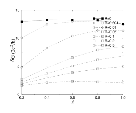
FIG. 6.: Difference $\delta G$ between maxima and minima in the conductance as a function of the parameter $\tilde{\epsilon}$, which characterizes the junction scattering matrices (realized by first method mentioned in text). Results are plotted for varying probabilities $R=|r_{N}|^{2}$ for normal reflection at the superconducting mirrors. The number of transverse modes are $N_{\perp}=40$. The results agree with the weak coupling limit calculated analytically, see Eq. (58).

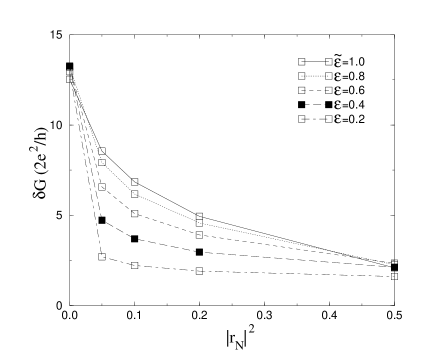
FIG. 7.: Difference $\delta G$ between maxima and minima in the conductance as a function of the probability $R=|r_{N}|^{2}$ for normal reflection at the superconducting mirrors (same data as in Fig. 6). The results agree with the weak coupling limit calculated analytically, see Eq. (58).

The second type of realization of the scattering matrix was done with Büttiker matrices [45] describing a coupling mode by mode between sample and reservoirs. In this case an additional unitary matrix was used, which only mixed the modes, see Appendix A. Both matrices were parametrized by the coupling parameter $\tilde{\epsilon}$. The result of these calculations are shown in Figs. 8-10. The only parameter to be changed in order to get different realizations of the random scattering matrix was an angle $\varphi_{ii}$ which only changed the position of the resonant peak. For zero angle the shape of the peak is seen in Fig. 11. The number of open modes are in this realization equal to the size of the matrix as all eigenvalues have an amplitude of unity.

The main result from the analytical calculations to be compared with the numerical results is $G_{max}-G_{min}$. This is in general approximately equal to $G_{max}$. From equation (45) we get

$$G_{max}\propto N_{\perp}\frac{2e^{2}}{h}\frac{\epsilon_{r}}{|r_{N}|}\quad$$ (65)

which agrees with numerical results when $\epsilon_{r}<|r_{N}|$.

The first realization of the random scattering matrix has been found to describe the weak coupling case as the observed peaks were narrow even for $\tilde{\epsilon}=1$. The second realization with a separate matrix mixing modes gave the possibility to study weak and intermediate coupling and the amplitude of oscillations were seen to diminish when $\tilde{\epsilon}$ was increased, see Fig. 11.

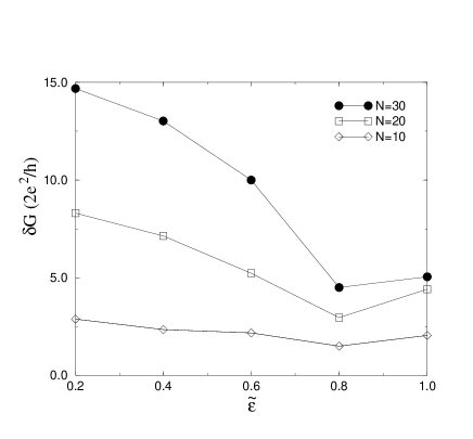
FIG. 8.: Difference $\delta G$ between maxima and minima in conductance as a function of coupling $\tilde{\epsilon}$ (scattering matrix realized by second method, see text). The probability for normal reflection $|r_{N}|^{2}=0$. The results agree with the analytical results in the weak and intermediate range of coupling where the resonant peak is proportional to the number of channels.

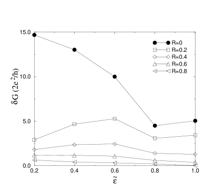
FIG. 9.: Difference $\delta G$ between maxima and minima in conductance as a function of coupling $\tilde{\epsilon}$. The number of open transverse modes are $N_{\perp}=30$. The results agree with Eq. (58) for weak coupling. For strong coupling the giant effect vanishes in a 2D sample according to the discussion in Section I.

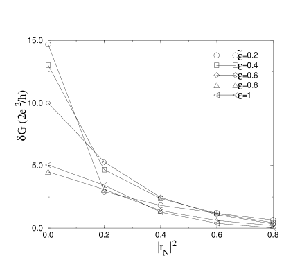
FIG. 10.: Difference $\delta G$ between maxima and minima in conductance as a function of normal reflection probability $|r_{N}|^{2}$ (same data as in Fig. 9). The number of open transverse modes is $N_{\perp}=30$, results for different strength of the coupling are shown. The results agree with analytical calculations. The $|r_{N}|^{2}$-dependence agress with Eq. (58).

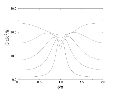
FIG. 11.: The resonance peaks at zero probability for normal reflection at the N-S boundaries. The results are from numerical calculations with $N_{\perp}=30$ and for different strength of coupling $\tilde{\epsilon}=[0.2,0.4,0.6,0.8,1.0]$ where the most narrow peak is for weakest coupling $\tilde{\epsilon}=0.2$. Note that the amplitude of oscillation is much larger than the conductance quantum even for $\tilde{\epsilon}=1$. This is because quasiparticle waves may pass the junction in our realization of the scattering matrix even if $\tilde{\epsilon}=1$.

VI Giant conductance oscillations for a diffusive normal sample - Feynman path integral approach.

In this Section we want to study the conductance oscillations by considering the probability amplitude for transmission and reflection of electrons and holes between the reservoirs via an S-N-S system the diffusive transport regime (see Fig. 1) as a sum of Feynman paths. [46] As we will show below, one does not actually need to do any complicated summations to find this probability amplitude, because for electron energies below the Thouless energy $E_{c}$ (or equivalently for temperatures below the Thouless temperature $T_{c}=E_{c}/k_{B}$) the hole exactly retraces the electron diffusive path after Andreev reflection. It follows that the phase gain of the electron along any resonant path between the N-S boundaries (see Fig. 1) is compensated by the hole phase gain along the same path. Therefore the phase gain is determined only by the phases imposed on the quasiparticles by the superconductors when a trajectory encounters the N-S boundaries. As a result the amplitude does not depend on either the form, the length of the diffusive path between the superconductors or the configuration of impurities (which means there is no need to perform any ensemble averaging of the conductance). The dependence of the resonant probability amplitude on the phase difference between the superconductors and on the scattering amplitudes at the barriers is easily found by calculating the number of reflections at the N-S boundaries and the number of backscattering events at the barriers. The conductance is equal to the probability of transmission (the modulus squared of the probability amplitude) multiplied by the number of different classical resonant paths (more strictly, by the number of tubes of width $\sim\lambda_{F}$ around these paths [46]) starting out from a reservoir lead; a number that can be straightforwardly estimated. We emphasize again that since the conductance associated with resonant transmission and reflection does not depend on the impurity configuration there is no need to average it with respect to the impurity positions.

We start by deriving an equation that connects the Feynman path integrals for electrons and holes. To do this we shall need the boundary conditions at an N-S boundary for the relevant Green’s functions.

The probability amplitude $K^{(e,h)}({\bf r},{\bf r}^{\prime};t-t^{\prime})$ for an electron (hole) to propagate from point ${\bf r}$ at time $t$ to point ${\bf r}^{\prime}$ at time $t^{\prime}$ is given by the time dependent Green’s function satisfying the following equation

$$\left(\mp i\hbar\partial/\partial t+\hat{H}\right)K^{(e,h)}({\bf r},{\bf r}^{\prime};t-t^{\prime})=\delta({\bf r}-{\bf r}^{\prime})\delta(t-t^{\prime})\;.$$ (66)

Here the plus (minus) sign is for electrons (holes). The initial condition is

$$K^{(e,h)}({\bf r},{\bf r}^{\prime};t-t^{\prime})=0\;\;\mbox{for}\;\;t-t^{\prime}<0$$ (67)

and$\hat{H}$ in Eq. (66) is the Hamiltonian describing a metal in the diffusive transport regime:

$$\hat{H}=-(\hbar/2m)\nabla^{2}+V_{imp}({\bf r})-\epsilon_{F}.$$ (68)

The potential $V_{imp}$ is

$$V_{imp}({\bf r})=\sum_{j}v({\bf r}-{\bf R}_{j}),$$ (69)

and $v({\bf r}-{\bf R}_{j})$ is the potential of an impurity at point ${\bf R}_{j}$.

In order to derive the boundary conditions we observe that the time Fourier transform of $K^{(e,h)}({\bf r},{\bf r}^{\prime};t-t^{\prime})$ for the case of electrons satisfies the equation

$$(\hat{H}-E-i\eta)K^{(e)}_{E}({\bf r},{\bf r}^{\prime})=\delta({\bf r}-{\bf r}^{\prime})$$ (70)

while for the hole case the equation is

$$(\hat{H}+E+i\eta)K^{(h)}_{E}({\bf r},{\bf r}^{\prime})=\delta({\bf r}-{\bf r}^{\prime})$$ (71)

($\eta$ is a small positive constant). At the N-S boundaries the Green’s functions $K^{(e,h)}_{E}({\bf r},{\bf r}^{\prime})$ are connected with each other by the Andreev reflection condition for a fixed energy:

$$K^{(h)}_{-E}({\bf r}^{(1,2)},{\bf r}^{\prime})=e^{i(\Phi_{1,2}+\Psi_{E})}K^{(e)}_{E}({\bf r}^{(1,2)},{\bf r}^{\prime})\;.$$ (72)

Here ${\bf r}^{(1,2)}$ and $\Phi_{1,2}$ are the coordinate and the phase of the gap function at the first (second) N-S boundary, respectivly, and ${\rm e}^{i\Psi_{E}}=|\Delta|/(E-i\sqrt{|\Delta|^{2}-E^{2}})$, where $|\Delta|$ is the magnitude of the gap. Now, an inverse Fourier transformation of Eq. (72) results in the following relation,

$$K^{(h)}({\bf r}^{(1,2)},{\bf r}^{\prime};\tau) = {\rm e}^{i\phi_{1,2}}\int_{-0}^{\infty}d\tau^{\prime}K_{E}^{(e)}({\bf r}^{(1,2)},{\bf r}^{\prime};\tau^{\prime})$$ (74)

$$\times\int_{-\infty}^{\infty}dE{\rm e}^{i\Psi_{E}}e^{i(\tau^{\prime}-\tau)E/\hbar}$$

where $\tau=t-t^{\prime}$. We are interested in the case when the characteristic time of transmission $t_{2}-t_{1}$ is of the order of the time, $L^{2}/D$, it takes to diffuse the length $L$ of the sample. Since this time can be expressed in terms of the Thouless energy as $\hbar/E_{c}$, the characteristic time difference $|\tau-\tau^{\prime}|$ in the last integral of Eq. (74) is of the order of $L^{2}/D=\hbar/E_{c}$. Therefore [47] in the last integral of Eq. (74) the main contribution is from energies inside an energy interval of order $E_{c}\ll|\Delta|$. In this interval $\Psi_{E}\approx\pi/2$ and hence the second integral in Eq. (74) is a Dirac $\delta$-function. Therefore the boundary condition for the time-dependent electron- and hole Green’s functions at the N-S boundaries is

$$K^{(h)}({\bf r}^{(1,2)},{\bf r}^{\prime};\tau)=e^{i(\phi_{1,2}+\pi/2)}K^{(e)}({\bf r}^{(1,2)},{\bf r}^{\prime};\tau)$$ (75)

According to the Feynman approach [46] a probability amplitude can be written as a path integral. Here we are interested in the following probability amplitude,

$$K({\bf r}_{1},t_{1};{\bf r}_{2},t_{2})=\int_{({\bf r}_{1},t_{1})}^{({\bf r}_{2},t_{2})}e^{iS\{{\bf r}(t)\}/\hbar}D\{{\bf r}_{e}(t)\}D\{{\bf r}_{h}(t)\}$$ (76)

This expression sums over all possible paths of an electron which start from a point ${\bf r}_{1}$ in the first reservoir at time $t_{1}$ and end at a point ${\bf r}_{2}$ at time $t_{2}$ in either the first or second reservoir and of all possible hole paths that appear due to Andreev reflections at the N-S boundaries. For any path the classical action is

$$S=\int_{t_{1}}^{t_{2}}{\cal L}dt+\Psi_{A}\;,$$ (77)

where the phase $\Psi_{A}$ will be discussed below. The Lagrangian ${\cal L}$ for those sections of the path where the particle moves as an electron is

$${\cal L}=m\dot{{\bf r}}^{2}_{e}-V\left({\bf r}_{e}(t)\right)$$ (78)

For those sections of the path where the particle moves as a hole we have

$${\cal L}=-m\dot{{\bf r}}^{2}_{h}+V\left({\bf r}_{h}(t)\right)\;.$$ (79)

Here $m$ is the electron mass, ${\bf r}_{e}$ and ${\bf r}_{h}$ are the electron and hole coordinates, respectively, the potential is $V=V_{0}+V_{imp}$; $V_{0}$ describes the barriers between the sample and the leads to the reservoirs [$V_{imp}$ is defined in Eq. (69)]. While performing the integration in Eq. (76) one has to use the N-S boundary conditions for electron and hole trajectories given by Eq. (75). The boundary conditions results in an additional term $\Psi_{A}$, which depends on the macroscopic phases of the superconductors:

$$\Psi_{A}= (\pi/2+\phi_{1})P^{(1)}_{e}+(\pi/2+\phi_{2})P^{(2)}_{e}$$ (81)

$$+(\pi/2-\phi_{1})P^{(1)}_{h}+(\pi/2-\phi_{2})P^{(2)}_{h}$$

In this expression $P^{(1)}_{(e,h)}$ and $P^{(2)}_{(e,h)}$ count how many electron-hole (hole-electron) transformations that has occurred at the N-S boundaries for a certain trajectory.

Transport properties of a diffusive system are usually calculated in the semiclassical approximation, which implies (for instance) that the cross section for impurity scattering is larger than $\lambda_{B}^{2}$. We adopt this point of view when we now proceed to calculate the functional integral in Eq. (76). This means that the method of steepest descent is useful for performing the integration in Eq. (76), and hence classical trajectories that minimize the action Eq. (77) contribute to the integral. [46]

In order to get the probability amplitude for transmission of an electron having fixed energy $E$ from point ${\bf r}_{1}$ of reservoir 1 to point ${\bf r}_{2}$ of reservoir 1 or 2 at all times one has to sum all the relevant amplitudes at all times, that is to integrate the amlitude $K$ (multiplied by a factor $\exp(iE\tau/\hbar)$) with respect to time $\tau=t_{2}-t_{1}$. From this we conclude that the probability amplitude $A(E)$ for transmission (or reflection) is equal to

$$A(E)=\sum_{\{S\}}R(S)exp\left[\int_{({\bf r}_{1})}^{({\bf r}_{2})}p_{S}(s)ds/\hbar+\Psi_{A}(S)\right]\;,$$ (82)

where summation is with respect to classical trajectories $S$ that start at point ${\bf r}_{1}$ and end at point ${\bf r}_{2}$ in reservoirs along which an electron with energy $E$ reaches reservoir 2 (since an electron or a hole) starting from reservoir 1, or is reflected back into reservoir 1 (as an electron or a hole); $p_{S}(s)$ is the classical momentum as a function of the coordinate $s$ along trajectory $S$, being equal to the electron momentum $p_{e}$ and hole momentum $p_{h}$ at the electron- and hole sections of the trajectory $S$, respectively. $R(S)$ is a product of the probability amplitudes of reflection and transition at the barriers between the sample and the reservoirs that occur for the electron and hole along path $S$. $\Psi_{A}(S)$ is the phase gained along the path $S$ by Andreev reflections at the N-S boundaries. When counting the number of the trajectories one has to take into account the fact that the trajectories has to be considered as tubes with a width of the order of the de Broglie wavelength $\lambda_{dB}=h/p_{F}$ (see above).

Now we can calculate the probability amplitudes for an electron at the Fermi level with energy $E=0$ from one reservoir to be reflected as a hole back to the same reservoir and to be transmitted as an electron to the other reservoir via the diffusive normal metal part of the sample. It is crucial for the calculation that at $E=0$ under Andreev reflection the hole and electron momenta are equal but their velocities have equal magnitude but opposite signs. This means that the classical trajectories of the electron and hole that end and start at the same points at the N-S boundaries exactly repeat each other in both ballistic and diffusive samples (as the classical trajectory is uniquely determined by the starting point and the velocity of the particle). Hence it follows that for any classical trajectory with Andreev reflections, at $E=0$ the total classical action $\int_{({\bf r}_{1})}^{({\bf r}_{2})}p_{S}(s)ds/\hbar$ (which is the sum of the electron and hole actions) is equal to zero as the electron and hole momenta are equal ($p_{e}=p_{h}$) and the integrations are along the same trajectory but in opposite directions. Therefore the phase gain along such trajectories [see Eq. (82)] does not depend on either their form, the length of the diffusion path or on the configuration of impurities. For resonant transmission the summation in Eq. (82) with respect to the ampencondlitude scatterings at the junctions is easily carried out in the case of low transparency of the barriers at the junctions.

The conductance of a hybrid sample containing both normal metal and superconductors, the normal conductance is determined [48] by the Landauer-Lambert formula (6), which for a symmetric system reduces to [7]

$$G=\frac{2e^{2}}{h}(T_{0}+R_{A})$$ (83)

The probabilities $T_{0}$ and $R_{A}$ were defined above [cf. Eq. (6)]. It is important to note that trajectories which connect the two reservoirs, necessarily have a different number of electron- and hole sections, while for trajectories which start and end in the same reservoir these numbers are equal. This is a crucial circumstance when one sums amplitudes in order to get the total transmission amplitude and implies that there is no complete compensation of the electron and hole phase gains along those trajectories which contribute to the transmission amplitude of quasiparticles. As a result destructive interference suppresses the transmission amplitude, and the main contribution to the conductance is from those trajectories along which the electron is reflected back into the same reservoir as a hole. This is the channel to be discussed below. A classical path corresponding to this type of reflection is shown in Fig. 1.

After passing the beam splitter at junction $A$ (that is after tunneling through the barrier of this junction) the classical diffusive electron trajectory can first encounter either the left N-S boundary (clockwise motion) or the right N-S boundary (counter-clockwise motion). Adding the amplitudes of clockwise and counter-clockwise trajectories (they form a geometric series) and expanding the amplitudes in $\delta\phi=\phi-\pi\ll 1$ one finds the total probability for an electron being reflected back into the same reservoir as a hole to be

$$R_{A}=\frac{\gamma^{2}\delta\phi^{2}}{(\gamma^{2}+\delta\phi^{2})^{2}}\;.$$ (84)

Here $\gamma\ll 1$ is the probability to pass through the barrier at the junction.

From Eq. (84) it follows that the electron-hole backscattering amplitude is zero if $\phi=\pi$. This is due to the interference between the clockwise and counter-clockwise quasiparticle trajectories (in the sense discussed above) and can be explained as follows. The amplitude of the electron-hole backscattering can be represented as a sum of contributions arising from trajectories with different number of Andreev reflections at the superconductors. The ratio between successive terms in this geometric series is equal to the amplitude of one Andreev reflection at each of the two N-S boundaries. Therefore it depends on the phase difference between the superconductors and becomes equal to one at resonance, when trajectories with very large number of Andreev reflections give the same contribution as the ones containing only few Andreev events. This is of course the reason why a resonance in the electron-hole backscattering channel occurs. In addition all terms in the series will be multiplied by a factor ${\rm e}^{i\phi_{s}}$ where $s$ labels the N-S boundary from which the electron first is Andreev reflected. In our notation $s=1$ for clockwise trajectories and $s=2$ for counter-clockwise trajectories. An important consequence of the existence of these multipliers is that on resonance, when $(\phi_{1}-\phi_{2}=\pi)$, the ratio of this extra exponents for clockwise and counterclockwise trajectories is equal to $-1$ and the resonant contributions from clockwise and counterclockwise trajectories to the amplitude for electron-hole backscattering cancel each other. A visible manifestation of this cancellation effect is a splitting of the resonant conductance peak near $\phi=\pi$ so that $G(\phi=\pi)=0$. [49]

If there are Schottky barriers at the N-S boundaries additional multipliers appear in the amplitudes for clockwise and counterclockwise trajectories. These are $r_{A}^{(s)}{\rm e}^{i\psi_{s}}$ ($r_{A}^{(s)}$ is the amplitude of Andreev reflection at the $s$:th N-S boundary ($s=1,2$)).

In the case of non-equivalent barriers, $r_{A}^{(1)}\neq r_{A}^{(2)}$, there is no compensation of the clockwise and counterclockwise contributions as is the case when $r_{A}^{(1)}=r_{A}^{(2)}$=1. In fact, if $r_{A}^{(1)}\ll r_{A}^{(2)}$ the splitting of the resonant peak disappears.

FIG. 12.: The resonant conductance peaks are split due to interference between clockwise and counter-clockwise quasiparticle motion along the trajectories that are associated with the formation of Andreev levels. Cf. Eq. (76); here $\gamma$ is 0.05 and 0.2.

In the semiclassical approximation the total number of electrons that contribute to the resonant phase-sensitive conductance is equal to the number $N_{\perp}$ of semiclassical tubes of diameter $\lambda_{F}$ that cover the cross-section of a lead between the reservoir and the diffusive sample (assuming the lead has a smaller cross section than the N-S boundaries). Hence from the Lambert formula (83) and Eq. (84) it follows that in the semiclassical approximation the phase-sensitive resonant conductance for a diffusive sample is equal to

$$G=(2e^{2}/h)N_{\perp}\frac{\gamma^{2}\delta\phi^{2}}{(\gamma^{2}+\delta\phi^{2})^{2}}$$ (85)

Equation (85) implies that the resonant conductance peaks are split in such a way that the conductance goes to zero when $\phi$ is an odd multiple of $\pi$ (see Fig. 12). This splitting appears due to the interference between the clockwise and counte-clockwise motion of the particles inside the normal sample when electrons are reflected as holes back to the same reservoir (see above).

The above calculations give a qualitative explanation to analytical and numerical results for the diffusive case presented in Refs. [13, 14, 19, 20, 21, 22, 24] if the results are obtained for low barrier transparency of the junctions between the sample and the reservoirs.

It should be noted that for the geometry considered in some of the papers cited above, where there is only one reservoir present, the conductance is determined only by the probability for an electron to be scattered back into the reservoir as a hole. Therefore the conductance is determined by the same equation (85) and hence must also be equal to zero at $\phi$ equal to odd multiples of $\pi$ for the equivalentN-S barrier case. The splitting must disappear for nonequivalent barriers at the N-S boundaries (see, e.g., Fig. 6 and Fig. 7 in Ref. [24]; a decrease of the barrier transparency at the junction between the sample and the reservoir results in the conductance peaks being close to those shown in Fig. (12) of this paper).

We conclude this Section by using the Feynman path integral approach to qualitatively consider the temperature dependence of the oscillating part of the conductance for the diffusive case and for temperatures above the Thouless temperature $E_{c}/k_{B}$. If the energy of an electron-hole excitation is not equal to zero there is no exact compensation of the phases gained along the electron- and hole portions of the paths connected by Andreev reflections. In this case the phase of the transmission amplitude $A$ depends on the lengths of the electron-hole paths, which in their turn depend on the starting points inside the lead between sample and reservoir. The conductance of the system is a sum of absolute squares of amplitudes corresponding to trajectories with different starting points in the lead for the classical paths. On the other hand classical paths starting from points separated by a distance greater than $\lambda_{F}$, meet different random sets of impurities [50]. As a result their path lengths have random values. Hence it follows that one can change the summation over starting points to a summation over path lengths when calculating the averaged conductance. For this purpose we assume a Gaussian length distribution of the diffusive paths that start at one N-S boundary and end up at the other N-S boundary (we choose the Gaussian form of the distribution function as an example; simple considerations show that choosing a more general distribution function only results in additional factors of order unity),

$$F({\cal L})=\frac{1}{\sqrt{\pi}{\cal L}_{0}}\exp\left(-\frac{{(\cal L}-{\cal L}_{0})^{2}}{{\cal L}_{0}^{2}}\right).$$ (86)

Here ${\cal L}_{0}$ is the average length of the paths (${\cal L}_{0}=L^{2}v_{F}/D$) . By averaging the conductance at a fixed energy over random path lengths described by the distribution function (86) one easily finds a cut-off factor of order $\exp\left(-[E/E_{c}]^{2}/4\right)$ appearing in the interference terms of the conductance. Therefore, destructive interference sets in at $E\gg E_{c}$ (this well known fact justifies the form of the distribution function assumed above). The conductance oscillations caused by interference only occur for energies below or of the order of $E_{c}$. As a result, at temperatures $T\gg E_{c}/k_{B}$ the amplitude of the conductance oscillations decreases with the temperature as $E_{c}/T$ in agreement with Refs. [2, 8, 9].

In order to find the temperature dependence of the giant conductance oscillations discussed here when $T\gg E_{c}/k_{B}$ and for low junction barrier transparencies we sum over the paths contributing to the resonance effect at a certain energy $E$, average the conductance over the path lengthsusing the distribution function (86) and integrate over energy taking the factor $(-\partial f_{0}/\partial E)$ properly into account ($f_{0}$ is the Fermi function). As a result we find that the oscillating part of the conductance caused by the resonant effect is

$$\delta G_{res}=N_{\perp}\frac{e^{2}}{h}\frac{\epsilon_{r}E_{c}}{k_{B}T}g(\phi)$$ (87)

Here $\epsilon_{r}$ is the transparency of the barrier at the junction, $g(\phi)$ is a $2\pi$-periodic temperature independent function with an amplitude of order unity.

The physical reason for the result (87) is that the position of the resonant energy peak is tuned by the superconducting phase difference $\phi$. With a change of $\phi$ it can be inside or outside the energy interval of order $E_{c}$ associated with the conductance oscillations. As the width of the resonant peak is $\delta E\sim\epsilon_{r}E_{c}$ the main contribution to the conductance oscillations comes from the energy interval $E\sim\epsilon_{r}E_{c}$, and hence the relative number of quasuparticles contributing to the oscillations is $\epsilon_{r}E_{c}/k_{B}T$. This is why this factor appears in Eq. (87).

VII Conclusions

In this paper we have presented a more thorough discussion than in a previous short communication [18] of giant conductance oscillations in hybrid mesoscopic systems of the Andreev interferometer type, i.e. S-N-S structures where the N-part is connected to normal electron reservoirs. In Ref. [18] giant conductance oscillations were predicted for a ballistic normal sample when transverse mode mixing was absent. The origin of this effect is a degeneracy (“bunching” effect) of the Andreev energy levels at the Fermi energy. This degeneracy of the Andreev spectrum arises due to an equality of the longitudinal momenta of Fermi energy electrons and -holes undergoing Andreev reflection. Any process that violates this equality lifts the degeneracy and, therefore, decreases the amplitude of the conductance oscillations.

In this paper we considered the effect of giant conductance oscillations taking into account transverse mode mixing at the junctions between the normal part of the sample and the reservoirs. We also considered normal reflection in addition to Andreev reflection at the N-S boundaries, and scattering of electrons and holes by impurities inside the normal sample.

Normal reflection of quasiparticles at N-S boundaries decreases the propability of Andreev reflection and as a consequence also decreases the amplitude of the conductance oscillations. We have shown that the probability amplitude for the oscillations is giant (that is proportional to the number of transverse modes $N_{\perp}$) until the amplitude of the normal reflection is smaller or of the same order as the transparency $|\epsilon_{r}|$ of the barriers at the junctions.

We have also shown that giant oscillations survive in a diffusive sample at temperatures much lower than the Thouless temperature. This is because after the electron-hole transformation associated with an Andreev reflection the electron and the hole move along the same classical diffusive trajectory in opposite directions but with equal momenta. As a result the phase gain of the electron and the hole along this diffusive path compensate each other. The probability amplitude for transmission through the sample does not depend on the form or the length of the diffusive path, but only on the phase difference between the superconductors (i.e., there is no destructive interference). The number of all possible different semiclassical paths is $S/\lambda_{B}^{2}=N_{\perp}$, where $S$ is the cross-section area, as each path has a width of the order of the de Broglie wave length $\lambda_{B}$. Therefore the amplitude of the conductance oscillations in the diffusive case remains giant and proportional to the number of transverse modes $N_{\perp}$ as for ballistic samples. The above qualitative picture agrees with analytical calculations for the diffusive case by Beenakker et al. [15], Zaitsev [14], Allsopp et al. [21], Volkov and Zaitsev [24], and Claughton et al. [23].

The presence of potential barriers at the junctions between the sample and the normal electron reservoirs is most crucial for the giant oscillations to exist. In the weak coupling case ($\epsilon_{r}\ll 1$) we have shown analytically and numerically that the amplitude of the conductance oscillations is independent of the barrier transparency and proportional to the number of transverse modes $N_{\perp}$. When the transparency of the barriers is increased, our numerical calculations show that the amplitude decreases. In the absence of barriers at the junctions the amplitude becomes zero. The latter result agrees with the sum rule in Ref. [21] according to which the conductance is equal to the number of transverse modes — in the absence of barriers — times the conductance quantum and does not depend on the superconducting phase difference. This can be qualitatively understood since an electron (hole) coming from the reservoir after being first Andreev reflected at one N-S boundary as a hole (electron) then at zero temperature returns to the reservoir by retracing the path of the incoming particle without reaching the second N-S boundary.

Recently Nazarov and Stoof [8], and Volkov et al. [9] proposed a new mechanism for conductance oscillations in diffusive samples that is effective if the temperature is close to the Thouless temperature (thermal effect). They used the dependence of the diffusion coefficient on the quasiparticle energy and found conductance oscillations with the superconducting phase difference in the absence of barriers. The amplitude of the oscillations was found to reach its highest value at the Thouless energy. We propose that this effect can be qualitatively understood if one takes into account the fact that under Andreev transformation at an N-S boundary there is a finite angle between the trajectories of the incident- and reflected particle, which is proportional to their excitation energy. Simple estimations show that near the Thouless temperature the classical trajectories of the electron and the hole can be separated by a distance of the order of the de Broglie wavelength (that is the width of the semiclassical trajectories) before the particle leaves the normal diffusive part of the sample for a reservoir. When this happens the trajectories meet different sets of impurities and can diffuse along very different paths inside the sample. This permits the quasi-particles to encounter also the other N-S boundary and undergo Andreev reflection there before leaving the sample. Therefore the conductance starts to depend on the superconducting phase difference and conductance oscillations arise. When the temperature is higher than the Thouless temperature, the phase gains of the quasi-particles along the semiclassical paths are not compensated and are much larger than unity; the destructive interference kills the thermal effect, in agreement with the results of the papers cited above.

When the transparency of the barriers at the junctions has intermediate values both the thermal effect and the resonant oscillation effect considered in this paper are in effect simultaneously provided the temperature is near the Thouless temperature. The effects can be distinguished by decreasing the temperature, which results in a decrease of the amplitude of the conductance oscillations in the case of the thermal effect (vanishing at zero temperature) while the resonant amplitude of the conductance increases and has its largest value at zero temperature.

This work was supported by the Swedish Royal Academy of Sciences (KVA) and by the Swedish Natural Science Research Council (NFR).

APPENDIX

A Elements of the scattering matrix describing coupling

We are to describe leads of finite width and the scattering matrix should mix different modes. The $S$ matrix will then be of size $3N_{\perp}\times 3N_{\perp}$ and the unitary condition for the submatrices of size $N_{\perp}\times N_{\perp}$ gives

$$\hat{s}_{11}\hat{s}_{11}^{{\dagger}}=1-2\hat{s}_{12}\hat{s}_{12}^{{\dagger}}\quad$$ (88)

$$\hat{s}_{22}\hat{s}_{22}^{{\dagger}}+\hat{s}_{23}\hat{s}_{23}^{{\dagger}}=\hat{1}-\hat{s}_{12}\hat{s}_{12}^{{\dagger}}\quad$$ (89)

$$\hat{s}_{22}\hat{s}_{23}^{{\dagger}}+\hat{s}_{23}\hat{s}_{22}^{{\dagger}}=-\hat{s}_{12}\hat{s}_{12}^{{\dagger}}\quad$$ (90)

$$\hat{s}_{11}s_{12}^{{\dagger}}+\hat{s}_{12}\left(\hat{s}_{22}^{{\dagger}}+\hat{s}_{23}^{{\dagger}}\right)=0\quad$$ (91)

$$\hat{s}_{12}\hat{s}_{11}^{{\dagger}}+\left(\hat{s}_{22}+\hat{s}_{23}\right)\hat{s}_{12}^{{\dagger}}=0\quad$$ (92)

Hence we have 5 matrix equations for 8 matrices (as each matrix has an independent hermitian and antihermitian part) there are 3 undetermined matrices. We choose them to be $\hat{s}_{12}$ and the antihermitian part of $\hat{s}_{22}$.

As it was said above the antihermitian part is not determined by the unitary conditions for the matrix $\hat{S}$. In general case it is of the same order of magnitude as the hermitian part as they are connected with the Kramers-Kronig relation. Therefore the matrix elements of $\hat{s}_{22}\propto\epsilon_{r}$. An analogous analysis of the rest of the equations shows the matrix elements of $\hat{s}_{23}-\hat{1}$, $\hat{\rho}_{11}$ and $\hat{V}$ to be of the same order of magnitude.

If $\hat{s}_{12}$ and the anti-hermitian part $\hat{s}_{22}^{(A)}$ commutes and other matrices are expressed in terms of $\hat{s}_{12}$ they may be simultaneously diagonalized. The $N_{\perp}$ eigenvalues of matrices $\hat{s}_{ij}$ are denoted $\lambda_{ij}$ were indices numbering the eigenvalues are suppressed. Directly from the unitary conditions we get

$$|\lambda_{11}|=\sqrt{1-2|\lambda_{12}|^{2}}$$ (93)

$$|\lambda_{23}|=\sqrt{1-|\lambda_{12}|^{2}-|\lambda_{22}|^{2}}$$ (94)

$$\lambda_{11}^{*}\lambda_{12}+\lambda_{12}^{*}(\lambda_{22}+\lambda_{23})=0$$ (95)

$$|\lambda_{12}|^{2}+2|\lambda_{22}||\lambda_{23}|\cos{(\phi_{22}-\phi_{23})}=0$$ (96)

which gives the requirement $\phi_{22}-\phi_{23}\in[\pi/2,3\pi/2]$. Now use a hermitian $\hat{s}_{12}$ i.e. real eigenvalues, $\phi_{12}=n\pi$. Put $\phi_{23}=0$ in order to agree with the weak coupling limit where no phase gain is expected in passing the reservoir. We get with $\lambda_{12}$ and $\lambda_{22}^{(A)}$ as eigenvalues of known hermitian matrices

$$|\lambda_{11}| = \sqrt{1-2|\lambda_{12}|^{2}}$$ (97)

$$\lambda_{11}^{(A)} = \lambda_{22}^{(A)}$$ (98)

$$\lambda_{11}^{(H)} = -\sqrt{|\lambda_{11}|^{2}-(\lambda_{11}^{(A)})^{2}}$$ (99)

$$\lambda_{11} = \lambda_{11}^{(H)}+i\lambda_{11}^{(A)}$$ (100)

$$\lambda_{22}^{(H)} = -{\lambda_{11}^{(H)}\over 2}+\sqrt{{(\lambda_{11}^{(H)})^{2}\over 4}+{|\lambda_{12}|^{2}\over 2}}$$ (101)

$$\lambda_{22} = \lambda_{22}^{(H)}+i\lambda_{22}^{(A)}$$ (102)

$$\lambda_{23} = \sqrt{1-|\lambda_{12}|^{2}-|\lambda_{22}|^{2}}$$ (103)

A symmetric random matrix with normally distributed elements will have real eigenvalues distributed according to the semicircle law. We have used values of mean 0 and variance 1 creating random matrices $\hat{s}_{12}$ and $\hat{s}_{22}^{(A)}$.

$$s^{(nm)}_{ij}=\langle{\phi_{n}}|\hat{s}_{ij}|{\phi_{m}}\rangle$$ (104)

where $|{\phi_{m}}\rangle$ is a complete set of vectors

$$\langle{\phi_{m}}|=\sum_{\alpha=1}^{N_{\perp}}\gamma_{\alpha}^{(m)}|{\psi_{\alpha}}\rangle$$ (105)

where $|{\psi_{\alpha}}\rangle$ are eigenvectors to $\hat{s}_{ij}$. If the corresponding eigenvalues are called $\lambda_{\alpha}$

$$s^{(nm)}_{ij}=\sum_{\alpha=1}^{N_{\perp}}\sum_{\beta=1}^{N_{\perp}}\gamma_{\alpha}^{(m)}\gamma_{\beta}^{(n)*}\langle{\psi_{\beta}}|\hat{s}_{ij}|{\psi_{\alpha}}\rangle=\sum_{\alpha=1}^{N_{\perp}}\gamma_{\alpha}^{(m)}\gamma_{\alpha}^{(n)*}\lambda_{\alpha}$$ (106)

With elements in the matrix $\hat{s}_{ij}$ of order unity

$$\sum_{\alpha=1}^{N_{\perp}}|\gamma_{\alpha}^{(m)}|^{2}=1$$ (107)

we get $\gamma_{\alpha}^{(m)}\propto 1/\sqrt{N_{\perp}}$. Our random matrix $\hat{s}_{12}$ will be multiplied by $\sqrt{\epsilon_{r}/N_{\perp}}$ before eigenvalues are calculated. Then by setting $\tilde{\epsilon}=\epsilon_{r}/\epsilon_{c}=1$ and approaching the strong coupling limit a maximum value $\epsilon_{c}$ is found fulfilling the unitary conditions. The strength of the coupling of the reservoirs is now parametrized by $\tilde{\epsilon}\in[0,1]$. The matrix $\hat{s}_{22}$ is in the weak coupling limit for one channel seen to be proportional to $\epsilon_{r}$ [45] and therefore the random matrix giving $\lambda_{22}^{(A)}$ is multiplied by $\epsilon_{r}/\sqrt{N_{\perp}}$. Then by using the eigenvectors of the matrix $\hat{s}_{12}$ we transform all the matrices $\hat{s}_{ij}$ back to the initial representation in which they are not diagonal and their matrix elements are the probability amplitudes of scattering to the respective transverse modes.

To realize another type of scattering matrix to describe the coupling to the reservoirs we do as follows. The essential features of the junction are coupling to electron reservoirs and mixing between modes, both features may be parametrized by the strength of the coupling $\tilde{\epsilon}$. The coupling to the reservoirs is described by Büttiker matrices. [45] If this is done mode by mode there will be no mixing. An additional unitary matrix is used to mix modes. This matrix has all diagonal elements equal to each other and all off-diagonal elements equal to each other, describing scattering into the same mode and mixing between modes respectively. By keeping the elements equal an isotropic situation is simulated where scattering into any mode is possible. The elements $u$ of the $N_{\perp}\times N_{\perp}$ unitary matrix must fulfill

$$|u_{ii}|^{2}+(N_{\perp}-1)|u_{ij}|^{2}=1$$ (108)

$$u_{ii}^{*}u_{ij}+u_{ij}^{*}u_{ii}+(N_{\perp}-2)|u_{ij}|^{2}=0$$ (109)

This gives $|u_{ij}|^{2}\leq 1/(N_{\perp}-1)$, the phases of $u_{ij}$ and $u_{ii}$ are connected by

$$\varphi_{ij}=\varphi_{ii}-\arccos\left(-\frac{(N_{\perp}-2)}{2}\frac{|u_{ij}|}{|u_{ii}|}\right)\\$$ (110)

we note that for $N_{\perp}>4$, $|u_{ij}|$ and $|u_{ii}|$ are not allowed to have the same value. We wish to consider large $N_{\perp}$ and write the elements

$${|u_{ii}|}^{2} = 1-c\tilde{\epsilon}$$ (111)

$${|u_{ij}|}^{2} = \frac{c\tilde{\epsilon}}{N_{\perp}-1}$$ (112)

in order to agree with the limit $\tilde{\epsilon}=0$ when mixing is expected to be absent since the waves in the decoupled sample do not feel the reservoirs. The condition Eq. (UnitaryU) gives

$$c=\frac{4(N_{\perp}-1)}{N_{\perp}^{2}}$$ (113)

The parameters are the coupling $\tilde{\epsilon}$, the number of modes $N_{\perp}$ and the angle $\varphi_{ii}$. We write the angle $\varphi_{ii}\in\tilde{\epsilon}[0,2\pi]$ to agree with the weak coupling limit where no phase gain is expected. By using different angles we get an ensemble of matrices describing different samples.

The eigenvalues of the unitary $\hat{U}$ all have amplitudes of length unity. This means that all modes will be open for transmission. [51] Opening of transmission channels has been observed in experiments. [25]

To describe coupling the results by Büttiker [45] are used in diagonal matrices. All these matrices $\hat{s}_{ij}$ are multiplied by $\hat{U}$.

B A barrier at the NS-interface

A Schottky barrier[42] at the interface of a semiconductor and a metal can be characterized with a scattering matrix

$$\hat{s}^{(0)}=-\left(\begin{array}[]{cc}r_{0}&t_{0}\\ -t_{0}^{*}&r_{0}^{*}\end{array}\right),\,\,\,\,\,\,|r_{0}|^{2}+|t_{0}|^{2}=1$$ (114)

that connects the constant factors $a_{1}$ and $b_{1}$ of the plane waves coming in and going out of the barrier inside the semiconductor, respectively, with those $a_{2}$ and $b_{2}$ inside the metal:

$$b_{i}=\sum_{k=1}^{2}s_{ik}^{(0)}a_{k},\,\,\,\,\,\,\ i=1,2$$ (115)

(Hence $|t_{0}|^{2}$ is the transparency of the barrier) When the metal is in the superconducting state the matrix of reflection of the semiconductor charge carriers at the N-S boundary (the semiconductor is on the right and the superconductor is on the left of the N-S boundary) is

$$\hat{\eta}=e^{i\Psi}\left(\begin{array}[]{ll}r_{N}&r_{A}\\ -r_{A}^{*}&r_{N}^{*}\end{array}\right)$$ (116)

where

$$e^{i\Psi}=i\frac{\sqrt{|t_{0}|^{4}+4|r_{0}|^{2}\sin^{2}\psi_{E}}}{e^{i\psi_{E}}-|r_{0}|^{2}e^{-i\psi_{E}}}$$ (117)

$$r_{N}=r_{0}^{*}\frac{2\sin\psi_{E}}{\sqrt{|t_{0}|^{4}+4|r_{0}|^{2}\sin^{2}\psi_{E}}}$$ (118)

$$r_{A}=it_{0}^{2}\frac{e^{i\phi}}{\sqrt{|t_{0}|^{4}+4|r_{0}|^{2}\sin^{2}\psi_{E}}}$$ (119)

$$e^{i\psi_{E}}=\frac{|\Delta|}{E-i\sqrt{|\Delta|^{2}-E^{2}}}$$ (120)

Here $|\Delta|$ and $\phi$ are the modulus and the phase of the superconducting gap, respectively, $E$ is the electron energy measured from the Fermi level. From Eq. (116-120) it is straightforward to see that $|r_{A}|^{2}+|r_{N}|^{2}=1$.

C Active channels

As for $N_{\perp}\gg 1$ the set of equations Eq. (27) can not be analytically solved and the amplitudes $\gamma_{n}$ can not be explicitly found we estimate the number $N_{R}$ of transverse modes inside the resonant region $(-\epsilon_{r}\hbar v_{F}/L,\epsilon_{r}\hbar v_{F}/L)$ and use Eq. (35) to get the conductance to within a factor of the order of unity. We determine $N_{R}$ in the following way.

$$N_{R}=\int\limits_{-\infty}^{\infty}dE\frac{\epsilon_{r}^{2}}{(EL/\hbar v_{F})^{2}+\epsilon_{r}^{2}}\nu(E)$$ (121)

where $\nu(E)$ is the state density function

$$\nu(E)=\sum\limits_{l}\sum\limits_{n=1}^{N_{\perp}}\delta(E-E_{n,l})=\sum\limits_{n=1}^{N_{\perp}}|\frac{\partial Q_{n}}{\partial E}|\delta(Q_{n});$$ (122)

Here the spectrum function $Q_{n}$ is determined by Eq. (51).

To find the state density function $\nu(E)$ we use the method developed in Ref. [52]. As $\frac{\partial\varphi_{-}}{\partial E}=\pm(\hbar v)^{-1}L$ with $v=\hbar\sqrt{k_{F}^{2}-k_{\perp}(n)^{2}}/m$ the factor $\partial Q_{n}/\partial E$ in (122) is a trigonometrical function of ${\pm}\varphi_{\pm}$ as well as $Q_{n}$ is, and it is productive to expand $\nu$ into Fourier series in $\varphi_{\pm}$ and write it as follows.

$$\nu(E)=\sum_{n=0}^{N_{\perp}}\sum_{s=-\infty}^{\infty}\sum_{k=-\infty}^{\infty}A_{s,k}e^{i(s\varphi_{-}+k\varphi_{+})}\quad$$ (123)

$$A_{s,k}=(2\pi)^{-2}\int_{0}^{2\pi}d{\bar{\varphi}}_{+}\int_{0}^{2\pi}d{\bar{\varphi}}_{-}|\frac{\partial Q_{n}}{\partial E}|\delta(Q_{n})e^{-i(s{\bar{\varphi}}_{-}+k{\bar{\varphi}}_{+})}\quad$$ (124)

In this paper we assume the length $L$ and the width $d$ of the sample to satisfy the inequality

$$\frac{d}{L}\gg\sqrt{\frac{\lambda_{F}}{L}}$$ (125)

Using this inequality, Eq. (133) and the estimation of Eq. (138) in Appendix D one sees that the main contribution to the state density function Eq. (122) is of the terms

$$A_{s,0} = \frac{L}{(2\pi)^{2}\hbar v}\int_{0}^{2\pi}d{\bar{\varphi}}_{+}\int_{0}^{2\pi}d{\bar{\varphi}}_{-}|\sin{\bar{\varphi}}_{-}|e^{-is{\bar{\varphi}}_{-}}$$ (127)

$$\times\delta(\cos{\bar{\varphi}}_{-}-|{r_{N1}}||{r_{N2}}|\cos{\bar{\varphi}}_{+}+|{r_{A1}}||{r_{A2}}|\cos\phi)$$

Performing integration with respect to ${\bar{\varphi}}_{-}$ in (127) and over $E$ in (121) with application of (123), (124) one obtains the conductance

$$G=N_{\perp}\frac{e^{2}}{2\pi\hbar}\epsilon_{r}\sum_{s=-\infty}^{\infty}e^{-2|s|\epsilon_{r}}\int_{0}^{2\pi}\cos s\varphi_{1}(\varphi_{+})d\varphi_{+}$$ (128)

$\displaystyle\varphi_{1}(\varphi_{+})=\arccos\Bigl{(}|{r_{N}}_{1}||{r_{N}}_{2}|\cos(\varphi_{+})-|{r_{A}}_{1}||{r_{A}}_{2}|\cos\phi\Bigr{)}$

if $0\leq\varphi_{-}\leq\pi$, and

$\displaystyle\varphi_{1}(\varphi_{+})=2\pi-\arccos\Bigl{(}|{r_{N}}_{1}||{r_{N}}_{2}|\cos(\varphi_{+})-|{r_{A}}_{1}||{r_{A}}_{2}|\cos\phi\Bigr{)}$

if $\pi\leq\varphi_{-}\leq 2\pi$. Performing summation in (128) one gets

$$G = N_{\perp}\frac{e^{2}}{\pi\hbar}\epsilon_{r}\times$$ (130)

$$\int_{0}^{2\pi}\frac{\epsilon_{r}d\varphi_{+}}{1-|{r_{N}}_{1}||{r_{N}}_{2}|\cos\varphi_{+}+|{r_{A}}_{1}||{r_{A}}_{2}|\cos\phi+\epsilon_{r}^{2}/2}$$

as $|{r_{N}}_{1,2}|\leq 1$ integration in (130) gives

$$G=N_{\perp}\frac{e^{2}}{\pi\hbar}\frac{\epsilon_{r}^{2}}{\sqrt{(1+|{r_{A}}_{1}||{r_{A}}_{2}|\cos\phi+\epsilon_{r}^{2}/2)^{2}-|{r_{N}}_{1}|^{2}|{r_{N}}_{2}|^{2})}}$$ (131)

If the boundaries are symmetric, that is ${r_{N1}=r_{N2}}$, the conductance is

$$G=N_{\perp}\frac{e^{2}}{\pi\hbar}\frac{\epsilon_{r}^{2}}{\sqrt{(1+|{r_{A}}|^{2}\cos\phi+\epsilon_{r}^{2}/2)^{2}-|{r_{N}}|^{4})}}$$ (132)

D Fast oscillating terms

In this Appendix we evaluate a sum of fast oscillating terms

$$S=\frac{1}{N_{\perp}}\sum\limits_{n=0}^{N_{\perp}}e^{iL[k_{F}^{2}-(\frac{\hbar}{d}n)^{2}]^{1/2}}$$ (133)

that appears in the density state function Eq. (122) and the transition probability Eq. (33), Eq. (34). Using the Poisson formula one can write

$$S=\lim\limits_{\delta\rightarrow 0}\frac{1}{N_{\perp}}\sum\limits_{k=-\infty}^{\infty}\ \int\limits_{0}^{N_{\perp}}dxe^{i\lambda\sqrt{1-x^{2}/\alpha^{2}}+i2\pi kx}e^{-\pi|k|\delta}$$ (134)

Here

$$\lambda=Lk_{F},\,\,\,\alpha=k_{F}d/\pi$$ (135)

As $\lambda\gg 1$ one can use the saddle point method to get

$$S = \frac{1}{N_{\perp}}\frac{\alpha}{\sqrt{\lambda}}\sqrt{\pi}e^{-i\pi/4}\times$$ (137)

$$\sum\limits_{k=-\infty}^{\infty}\left(\frac{\lambda^{2}}{\lambda^{2}+(2\pi\alpha k)^{2}}\right)^{3/4}e^{i\sqrt{\lambda^{2}+(2\pi\alpha k)^{2}}}$$

From Eq. (137) it follows that terms with $k$ which are less or of the order of $\lambda/\alpha$ contribute to the sum and, therefore, $S$ is less than $\sqrt{\lambda}/$ $N_{\perp}$. As $N_{\perp}\sim k_{F}d$ we have the following estimation of the sum of fast oscillating terms.

$$S\leq\sqrt{Lk_{F}}/\left(k_{F}d\right)$$ (138)

Therefore the sum of fast oscillating terms can be neglected if

$$\frac{d}{L}\gg\sqrt{\frac{\lambda_{F}}{L}}$$ (139)

REFERENCES

- [1] A. F. Andreev, Zh. Eksp. Teor. Fiz. 46, 1823 (1964); 51, 1510 (1966) [Sov. Phys. JETP 19, 1228 (1964); 24 , 1019 (1967)].
- [2] B. Z. Spivak and D. E. Khmel’nitsky, Pis’ma Zh. Eksp. Teor. Fiz. 35, 334, (1982) [JETP Lett. 35, 412 (1982)]; B. L. Altshuler and B. Z. Spivak, ibid. 92, 609 (1987) [65, 343 (1987)]; B. Z. Spivak and A. Yu. Zyuzin, in Mesoscopic Phenomena in Solids, edited by B. L. Altshuler, P. A. Lee, and R. A. Webb (Elsevier Science, New York, 1991), p.37.
- [3] H. Nakano and H. Takayanagi, Solid State Commun. 80, 997, 1991; H. Nakano and H. Takayanagi, Phys. Rev. B 47, 7986, 1993.
- [4] V. T. Petrashov, V. N. Antonov, P. Delsing, T. Claeson, Phys. Rev. Lett., 70, 347, 1993.
- [5] F. W. J. Hekking and Yu. V. Nazarov, Phys. Rev. Lett., 71, 1625, 1993.
- [6] V. C. Hui and C. J. Lambert, Europhys. Lett., 23, 203, 1993.
- [7] C. J. Lambert, J. Phys.: Cond. Matter, 3, 6579, 1991; J. Phys.: Cond. Matter, 5, 707, 1993; C. J. Lambert, V. C. Hui, S. J. Robinson, J. Phys.: Cond. Matter, 5, 4187, 1993.
- [8] Yu. V. Nazarov and T.H. Stoof, Phys. Rev. Lett. 76, 823, 1996.
- [9] A. Volkov, N. Allsopp and C. J. Lambert, J. Phys.: Condens. Matter 8, L45, 1996;
- [10] H. Pothier, S Guéron, D Estéve, M. H. Devoret, Physica B 203, 226, 1994; H.Pothier, S. Guéron, D. Estève, and M. H. Devoret, Phys. Rev. Lett. 73, 2488 (1994).
- [11] van Wees, B. J. Dimoulas, J. P. Heida, T. M. Klapwijk, W.v.d. Graaf, G. Borghs, Physica B 203, 285 (1994).
- [12] P. G. N. de Vegvar, T. A. Fulton, W. H. Mallison, and R. E. Miller, Phys. Rev. Lett. 73, 1416 (1994).
- [13] Yu. V. Nazarov, Phys. Rev. Lett. 73, 1420, 1994.
- [14] (a) A.V. Zaitsev, Physica B, 203, 274 (1994), (b) A.V. Zaitsev, Phys. Lett. A 194, 315 (1994).
- [15] C. W. J. Beenakker, J. A. Melsen, and P. W. Brouwer, Phys. Rev. B 51, 13 883 (1995).
- [16] V. T. Petrashov, V. N. Antonov, P. Delsing, and T. Claeson, Phys. Rev. Lett. 74, 5268 (1995).
- [17] N. R. Claughton, M. Leadbeater, C. J. Lambert, V. N. Prigodin, preprint cond-mat/9510117
- [18] A. Kadigrobov, A. Zagoskin, R. I. Shekhter and M. Jonson, Phys. Rev. B 52, R8662 (1995).
- [19] P. M. A. Cook, V. C. Hui and C. J. Lambert, Europhys. Lett. 30, 355 (1995).
- [20] N. R. Claughton. R. Raimondi and C. J. Lambert, Phys. Rev. B 53, 9310, 1996.
- [21] N. K. Allsopp, J. Sanchez Canizares, R. Raimondi and C. J. Lambert, J. Phys.: Condens. Matter 8, L377 (1996).
- [22] N. R. Claughton and C. J. Lambert, Phys. Rev. B 53, 6605, 1996.
- [23] N. R. Claughton, R. Raimondi, C. J. Lambert, Phys. Rev. B 53, 9310, 1996.
- [24] A. F. Volkov and A. V. Zaitsev, Phys. Rev. B 53, 9267, 1996.
- [25] L. C. Mur, C. J. P. M. Harmans, J. E. Mooij, J. F. Carlin, A. Rudra, M. Ilegems, Phys. Rev. B 54, R2327, 1996.
- [26] P. Charlat, H. Courtois, Ph. Gandit, D. Mailly, A. F. Volkov, B. Pannetier, preprint (cond-mat/9605021); (cond-mat/9609182).
- [27] S. G. den Hartog, C. M. A. Kapteyn, B. J. van Wees, T. M. Klapwijk, W. van der Graaf, G. Borghs, Phys. Rev. Lett. 76, 4592, 1996.
- [28] F. Rahman et al. Phys. Rev. B 54, 14026, 1996.
- [29] S. Ohki, Y. Ootuka, J. Phys. Soc. Jpn. 65, 1917, 1996.
- [30] B. J. van Wees, H. Takayanagi, Mesoscopic Transport, Eds. L. P. Kouwenhoven, G. Schön, L. L. Schön, Kluwer Academic Publ., Dordrecht, The Nederlands.
- [31] F. Zhou, B. Spivak, preprint (cond-mat/9604185).
- [32] V. T. Petrashov, R. Sh. Shaikhaidarov, I. A. Sosin, Pis‘ma Zh. Eksp. Teor. Fiz. 64, 789 (1996).
- [33] B. J. van Wees, P. de Vries, P. Magnee, and T. M. Klapwijk, Rhys. Rev. Lett. 69, 510 (1992).
- [34] H. Takayanagi, T. Akazaki, J. Nitta, Phys. Rev. Lett., 75, 3533, 1995; H. Takayanagi and T. Akazaki, Phys. Rev. B 52, R8633 (1995); H. Takayanagi, T. Akazaki, Jpn. J. Appl. Phys. 34, 6977, 1995.
- [35] Recent experiments [36, 37] show a distinct shift in the phase dependence from what is expected for the thermal effect (the conductance maxima appear for even multiples of ) to the pattern typical for the giant oscillation effect (the conductance maxima are at odd multiples of ) when the temperature is lowered. It is worth noticing that in cases where no Schottky barrier is expected at the junctions between sample and reservoirs some scattering is still caused by the junction geometry. In this situation backscattering is possible only from a region within a distance of order from the junction edges. Under this condition the zero-temperature amplitude is not giant in the sense used in this introduction, but it is nevertheless large.
- [36] V. T. Petrashov, R. Sh. Shaikhaidarov, I. A. Sosnin, P. Delsing and T. Claeson, (unpublished).
- [37] E. Toyoda and H. Takayanagi, (unpublished).
- [38] J. Nitta, T. Akazaki, H. Takayanagi, and K. Arai, Phys. Rev. B, 46, 14 286 (1992).
- [39] C. Nguyen, H. Kroemer, and E. L. Hu, Phys. Rev. Lett. 69, 2847 (1992).
- [40] A. Dimoulas, J. P. Heida, B. van Wees, T. M. Klapwijk, W. v.d. Graaf, and G. Borghs, Phys. Rev. Lett. 74, 602 (1995).
- [41] K. M. H. Lenssen, L. A. Westerling, P. C. A. Jeekel, C. J. P. M. Harmans, J. E. Mooij, M. R. Leys, W. van der Vlueten, J. H. Wolter, S. P. Beaumont, Physica B 194-196, 2413 (1994).
- [42] G. E. Blonder, M. Tinkham, T. M. Klapwijk, Phys. Rev. B 25, 4515 (1982).
- [43] I. O. Kulik, Zh. Eksp. Teor. Fiz. 57, 1745 (1969) [Sov. Phys. JETP 30, 944 (1970)].
- [44] Although in a given experiment the matrix elements are fixed and uniqely determined, they are sample dependent. We keep in mind that the conductance which we calculate should be ensemble averaged with respect to such uncontrollable variations. If in this procedure one formally considers this matrix to be random and its elements distributed around to satisfy the unitary conditions (88)-(92), then its eigenvalues will be distributed in the interval [-1, 1] according to the semicircle law [53]. Hence, in such an averaging procedure the most representative matrices would have eigenvalues of order unity.
- [45] M. Büttiker, Y. Imry, M. Ya. Azbel, Phys. Rev. A 30, 1982, 1984.
- [46] R. P. Feynman, A. R. Hibbs, Quantum Mechanics and Path Integrals, McGraw-Hill, 1965.
- [47] We assume that so that Andreev reflection is prominent on the energy scale given by . Physically this means that the distance between the superconductors is much larger than the penetration length into the normal metal of the superconducting correlations. In experiments this condition is easily satisfied since 0.1 K.
- [48] According to Lambert [7], when a voltage is applied between the reservoirs the chemical potential of the superconductors (the chemical potentials of the semiconductors and the normal part of the sample are equal) must be chosen self-consistently with the condition of conservation of the current outgoing from and incoming to the reservoirs via the sample. The superconductor chemical potential as a result lies between the chemical potentials of the reservoirs. Hence electrons are emitted from the reservoir with the higher chemical potential, and holes from the reservoir with the lower potential.
- [49] It interesting to note that this peak splitting takes place also for a ballistic sample. However, in this case, in contrast to the diffusive sample, the contribution to the conductance due to transmission of an electron to the second reservoir via the ballistic sample is not suppressed. As a result, in the general case for the ballistic system the conductance is not equal to zero at . However the value of the conductance at is controlled by the parameter ( is the distance between the junctions) and is equal to zero when (modulo ) [see the discussion at the end of Section III).
- [50] This means that for the transverse modes a summation with respect to starting points of the paths is equivalent to an impurity averaging of the conductance. This is a manifestation of the fact that the conductance is a self-averaging quantity.
- [51] Y. Imry, Europhys. Lett. 1, 249, 1986.
- [52] A. A. Slutskin, Zh. Eksp. Teor. Fiz., 58, 1098 (1970)
- [53] M. L. Mehta, Random Matrices, Academic Press, 1991.