Cumulant approach to the low-temperature thermodynamics of many-body systems

Abstract

Current methods to describe the thermodynamic behavior of many-particle systems are often based on perturbation theory with an unperturbed system consisting of free particles. Therefore, only a few methods are able to describe both strongly and weakly correlated systems along the same lines. In this article we propose a cumulant approach which allows for the evaluation of excitation energies and is especially appropriate to account for the thermodynamics at low temperatures. The method is an extension of a cumulant formalism which was recently proposed to study statical and dynamical properties of many-body systems at zero temperature. The present approach merges into the former one for vanishing temperature. As an application we investigate the thermodynamics of the hole-doped antiferromagnetic phase in high-temperature superconductors in the framework of the anisotropic $t$-$J$ model.

I Introduction

For the investigation of many-particle systems at finite temperatures the free energy $F$ plays a central role. One basic property of the free energy is its size consistency, i.e. the free energy scales with the size of the system. Each approximation which is used to evaluate $F$ must preserve this property. In diagrammatic approaches size consistency is guaranteed by the fact that in any physical quantity only linked diagrams enter. Usually, diagram technique makes use of Wick’s theorem, which is appropriate only if the unperturbed Hamiltonian is a single-particle Hamiltonian. Therefore standard diagrammatic approaches are restricted to weakly correlated systems. An alternative approach to evaluate statical and dynamical properties at zero temperature was recently proposed [1, 2, 3] and is based on the introduction of cumulants. As is well known from statistical physics the use of cumulants ensures size consistency. This favors the cumulant method especially for the description of strongly correlated systems though it may be applied as well to weakly correlated systems. The main aspect of the present paper is to investigate excitation energies which are needed to evaluate the free energy.

There is a natural danger that a cumulant expansion of $F$ is only valid for high temperatures. Expanding with respect to small values of the inverse temperature $\beta=1/kT$ the partition function reads

$$Z=Z\left(0\right)\langle 1-\beta H+\frac{1}{2}\beta^{2}H^{2}\cdots\rangle_{0}\,\,\,,$$ (1)

where $\langle\cdots\rangle_{0}=Tr(\dots)/Tr\,1$ stands for an unweighted average at infinite temperature and $Z\left(0\right)=Tr\,1$ is the trace of the unity operator $1$. Expanding $\ln{Z}$, suitably regrouped into contributions in powers of $\beta$, one finds for the free energy

$$F= -\frac{1}{\beta}\ln Z\left(0\right)+\langle H\rangle_{0}+\frac{1}{2}\beta\left[\langle H^{2}\rangle_{0}-\langle H\rangle^{2}_{0}\right]$$ (3)

$$+\frac{\beta^{2}}{3!}\left[\langle H^{3}\rangle_{0}-3\langle H^{2}\rangle_{0}\langle H\rangle_{0}+2\langle H^{3}\rangle_{0}\right]+\cdots\,\,\,,$$

Note that the expressions in the brackets $\left[\cdots\right]$ are cumulants.

In the present approach we want to avoid that a free energy expansion like (3) is only valid for high temperatures. Of more interest are low-temperature expansions. A low-temperature expansion for $F$ must reduce to the ground-state energy in the limit $T\rightarrow 0$. In contrast to a high-temperature expansion where $\beta$ is small, for sufficiently low temperatures the canonical weight $\exp\left(-\beta(E_{n}-E_{0})\right)$ is small for excitations $E_{n}$ higher than the ground-state energy $E_{0}$. Therefore, in case of a non-degenerate ground state the free energy can be expanded for low temperatures as follows

$$F = -\frac{1}{\beta}\ln{Z}=E_{0}-\frac{1}{\beta}\ln{(1+\sum_{n>0}e^{-\beta(E_{n}-E_{0})})}$$ (4)

$$= E_{0}-\frac{1}{\beta}(\sum_{n>0}e^{-\beta(E_{n}-E_{0})}+\cdots)$$ (5)

A neglection of high-lying excitations is not always allowed. For instance, for the one-dimensional Ising model in a longitudinal field the thermodynamic limit and the limit $T\rightarrow 0$ do not commute. This is an alternative description of the fact that long-range order is destroyed in one dimension.

In this paper we propose a cumulant formalism for the calculation of excitation energies of correlated electronic systems. This method is based on a perturbational approach, i.e., the Hamiltonian is splitted into $H_{0}$ and $H_{1}$ with $H_{0}$ being exactly solvable. One starts from eigenstates of $H_{0}$ and includes the effect of $H_{1}$ by an exponential ansatz. Especially for the zero-temperature version of the method this can be shown to be equivalent to summing a perturbation series to infinite order. So the present method is well suited for systems which can in principle be treated perturbatively, but it can not account for systems with very large fluctuations, e.g., most one-dimensional spin models.

This paper is organized as follows. In the Sec. II we shortly review the size-consistent ground-state version of the cumulant method. In Sec. III the cumulant method for the computation of excitation energies is presented. With this general scheme we are able to calculate partition functions. To demonstrate the applicability of the method we investigate the $t$-$J$ model at weak doping as a topic of current interest. We consider a two-dimensional model with anisotropic magnetic exchange and calculate the staggered magnetization within the antiferromagnetic phase in dependence on temperature and hole concentration. A discussion and concluding remarks are put in the last section.

II Review of the zero-temperature version of the cumulant method

For a better understanding of the cumulant method its ground-state version is briefly reviewed. For more details see[1, 2, 3, 4]. The method starts from the definition of the function

$$f\left(\lambda\right)=\ln\langle\phi_{0}|e^{-\lambda(H_{0}+H_{1})}e^{\lambda H_{0}}|\phi_{0}\rangle$$ (6)

where $H_{0}$ is the rigorously solvable unperturbed Hamiltonian $H_{0}$ with the ground state $|\phi_{0}\rangle$, i.e., $H_{0}|\phi_{0}\rangle=\epsilon_{0}|\phi_{0}\rangle$. The aim is to calculate the ground-state energy $E_{0}$ of the full system, $H|\psi_{0}\rangle=E_{0}|\psi_{0}\rangle$. The shift of the ground-state energy $\delta E_{0}=E_{0}-\epsilon_{0}$ due to the perturbation $H_{1}$ can be derived in a straightforward way. Introducing the Liouvillian $L_{0}$ which is defined by $L_{0}A=\left[L_{0},A\right]$ for any operator $A$, equation (6) is transformed into

$$f\left(\lambda\right)=\ln\langle\phi_{0}|e^{-\lambda(H_{1}+L_{0})}|\phi_{0}\rangle\,\,\,.$$ (7)

Next, we define the Laplace transform of the function $f\left(\lambda\right)$ by:

$$\hat{f}\left(z\right)=-\int\limits_{0}^{+\infty}\,f\left(\lambda\right)\,e^{\lambda\,z}\,dz\,\,\,,\hskip 56.9055pt\Re\{z\}<0\,\,\,.$$ (8)

One can show[1, 4] that the energy shift $\delta E_{0}$ with respect to the unperturbed ground-state energy $\epsilon_{0}$ is given by

$$\delta E_{0}=\lim_{z\rightarrow 0}z^{2}\hat{f}\left(z\right)\,\,\,.$$ (9)

On the other side, equation (7) is used to express $\delta E_{0}$ in terms of cumulants

$$\delta E_{0}=\lim_{z\rightarrow 0}\,\,\langle\phi_{0}|H_{1}\left(1+\frac{1}{z-H_{1}-L_{0}}H_{1}\right)|\phi_{0}\rangle^{c}\,\,\,.$$ (10)

Here $\langle\phi_{0}|...|\phi_{0}\rangle^{c}$ denotes cumulant expection values with respect to the unperturbed ground state $|\phi_{0}\rangle$. Cumulant expectation values[5] for a product of arbitrary operators $A_{i}$ with an arbitrary state $|\phi\rangle$ are defined by:

$$\langle\phi|\prod_{i}A_{i}^{n_{i}}|\phi\rangle^{c}\,=\,\left(\prod_{i}\left({\partial\over\partial\lambda_{i}}\right)^{n_{i}}\right)\ln\langle\phi|\prod_{i}{\rm e}^{\lambda_{i}A_{i}}|\phi\rangle\,|_{\lambda_{i}=0\,\forall\,i}\,.$$ (11)

For a note on generalized cumulants see Appendix A. The quantity inside the bracket of (10) is called wave operator $\Omega$ (it has similarity with the Möller operator known from scattering theory),

$$\Omega = 1+\lim_{z\rightarrow 0}\frac{1}{z-H_{1}-L_{0}}H_{1}\,.$$ (12)

Thus we can rewrite $\delta E_{0}$ as

$$\delta E_{0} = \langle\phi_{0}|H_{1}\Omega|\phi_{0}\rangle^{c}\ \ \ \ \ \mbox{or}\ \ \ E_{0}=\langle\phi_{0}|H\Omega|\phi_{0}\rangle^{c}$$ (13)

Within cumulants, the operator $\Omega$ transforms the ground state $|\phi_{0}\rangle$ of the unperturbed Hamiltonian $H_{0}$ into the full ground state $|\psi_{0}\rangle$ of $H$. Expanding (12) into powers of $H_{1}$ it can be shown that (13) is equivalent to Rayleigh-Schrödinger perturbation theory summed up to infinite order, see e.g. [4].

There is no general rule how to split $H$ into $H_{0}$ and $H_{1}$ except that the overlap between the unperturbed and the full ground state has to be non-zero, i.e., $\langle\psi_{0}|\phi_{0}\rangle\neq 0$. The operator $\Omega$ describes the influence of $H_{1}$ onto $|\phi_{0}\rangle$. This effect should be a small correction to $|\phi_{0}\rangle$, i.e., it should be treatable perturbatively in the sense that it can be obtained by summation of a perturbation expansion. This is usually fulfilled if $H_{0}$ is the dominant part of the Hamiltonian. Therefore, for strongly correlated systems $H_{0}$ should consist of the correlations (or at least part of them) whereas $H_{1}$ usually contains the hybridization. In the application presented in Sec. IV dealing with the weakly doped $t-J$ model $H_{0}$ contains the Ising part of the magnetic interaction whereas $H_{1}$ consists of its transverse part and the electron hopping. Other interesting examples may be found in refs. [6, 7]. If the full ground state $|\psi_{0}\rangle$ is expected to break a symmetry of $H$ then $H_{0}$ has to be chosen so that its ground state $|\phi_{0}\rangle$ breaks this symmetry, too.

Instead of using the explicit form (12) of the wave operator $\Omega$ an exponential ansatz was proposed [8]

$$\Omega=e^{S}\,,\quad S=\sum_{\mu}\alpha_{\mu}S_{\mu}$$ (14)

where $\{S_{\mu}\}$ is a set of relevant operators. They have to be chosen in such a way that $\exp(\sum_{\mu}\alpha_{\mu}S_{\mu})|\phi_{0}\rangle$ (with appropriate parameters $\alpha_{\mu}$) represents a good approximation of the exact ground state. The yet unknown parameters $\alpha_{\mu}$ are to be determined from the following set of equations

$$\langle\phi_{0}|S_{\nu}^{\dagger}H\Omega|\phi_{0}\rangle^{c}=0\,,\,\,\ \ \ \ \ \nu=1,2,3,\cdots$$ (15)

These equations follow from the condition of $\Omega|\phi_{0}\rangle$ being an eigenstate of $H$. Note that equations (13) and (15) allow for the computation of the ground-state energy. For algebraic reasons it is suitable to use operators $S_{\mu}$ which only create (but do not destroy) fluctuations with respect to the unperturbed ground state $|\phi_{0}\rangle$. Then the expansion of the exponential in (13) and (15) stops after a few terms because the Hamiltonian $H$ and the adjoint fluctuation operators $S_{\nu}^{\dagger}$ have to remove all fluctuations which are created by $\Omega$ and $H_{1}$ in the state $|\phi_{0}\rangle$.

The choice of appropriate operators $S_{\nu}$ is most important for actual calculations using the cumulant method. These operators describe fluctuations introduced into $|\phi_{0}\rangle$ by successive application of $H_{1}$. In principle, they can be derived systematically from the explicit form (12) of the wave operator $\Omega$. For practical applications this might be only of little help especially if the main physical effect comes from higher powers of $H_{1}$. In such a case a small set of few relevant operators leads to a far simpler description of the main effect than including a large set of powers $H_{1}^{n}$. The selection of relevant operators for the cumulant method can be seen similar to the selection of dynamical variables for Mori-Zwanzig projection technique: Formally, variables can be systematically derived from the Liouvillian, but often choosing variables from physical insight is more useful.

For a discussion of the cumulant method and its relation to other methods like variational calculations and the coupled-cluster method see appendix C. In the past, equations (13,15) was used to evaluate ground-state properties of several systems, see for instance [2, 6, 7, 9, 10, 11].

III Extension to finite temperatures

Now we present a cumulant scheme for calculating excitation energies. To discuss the influence of the perturbation $H_{1}$ we formally introduce an additional parameter $\lambda$ in the Hamiltonian:

$$H\;=\;H_{0}\,+\,\lambda H_{1}$$ (16)

As is shown below, the wave operator $\Omega$ from the zero-temperature approach will be replaced by a unitary operator $U$ which diagonalizes the full Hamiltonian $H$. The operator $U$ transforms all eigenstates of the unperturbed system into eigenstates of the full Hamiltonian. Being $|\phi_{n}\rangle$ and $|\psi_{n}\rangle$ the eigenstates of $H_{0}$ and $H$,

$$H_{0}|\phi_{n}\rangle=\epsilon_{n}|\phi_{n}\rangle\ \ ,\ \ \ \ \ \ \ \ \ H|\psi_{n}\rangle=E_{n}|\psi_{n}\rangle\,,$$ (17)

the action of $U$ is defined by

$$|\psi_{n}\rangle=U|\phi_{n}\rangle$$ (18)

with $U$ depending smoothly on $\lambda$ and $U\rightarrow 1$ for $\lambda\rightarrow 0$. Every unitary operator can be written as

$$U\>=\>e^{S}\quad\mbox{with}\quad S^{\dagger}\,=\,-S\,.$$ (19)

In general, the unitary transformation $U$ is not known for a given system. Therefore approximations for $U$ have to be used. Generalizing the exponential form (14) for the wave operator $\Omega$ from the zero-temperature approach to a unitary operator, we make the following ansatz

$$U=e^{S}\,,\quad S=\sum_{\mu}\alpha_{\mu}(S_{\mu}-S_{\mu}^{\dagger})$$ (20)

where both $S_{\mu}$ and the adjoint operators $S_{\mu}^{\dagger}$ are enclosed in the exponential. The $\{S_{\nu}\}$ form a set of relevant operators as in the zero-temperature approach. In most cases, using a finite number of operators $S_{\nu}$ represents an approximation of $U$. However, with the number of operators going to infinity the exact transformation $U$ can be approximated with arbitrary accuracy.

In contrast to the ground-state approach the operators $S_{\mu}$ and $S_{\mu}^{\dagger}$ can create and also annihilate fluctuations. This also means that the application of $(S_{\mu}-S_{\mu}^{\dagger})$ to an eigenstate $|\phi_{n}\rangle$ of $H_{0}$ (with energy $\epsilon_{n}$) leads to a new state which may overlap with eigenstates of $H_{0}$ having energies both below and above $\epsilon_{n}$.

In the finite-temperature approach the former equations (13) and (15) are replaced by

$$E_{n}\> = \>\langle HU\rangle_{n}^{c}\,,$$ (21)

$$0\> = \>\langle(S_{\nu}-S_{\nu}^{\dagger})^{\dagger}HU\rangle_{n}^{c}\,,\ \ \ \ \ \nu=1,2,3,\cdots$$ (22)

where $\langle\cdots\rangle_{n}^{c}$ refers to the cumulant average now formed with the unperturbed eigenstate $|\phi_{n}\rangle$ of $H_{0}$, i.e., $\langle\cdots\rangle_{n}^{c}=\langle\phi_{n}|\dots|\phi_{n}\rangle^{c}$. The parameters $\alpha_{\mu}$ can be determined from Eqs. (22). Note that the cumulants in (22) can be formed with any unperturbed eigenstate $|\phi_{n}\rangle$ of $H_{0}$ as long as the exact expression for the unitary transformation $U$ is known. However, for any approximation for $U$ the parameters $\alpha_{\mu}$ may vary with a different choice of the $|\phi_{n}\rangle$ used for the cumulant expectation values.

To prove Eqs. (21,22) one can either make use of a method recently proposed [12] which is based on integrating over infinitesimal transformations $(1+S/N)$. Here we rather prefer to make explicit use of the definition (11) of cumulant expectation values. Expanding $U=e^{S}$ in powers of $S$ and taking the definition (11) for cumulant expectation values one finds for the r.h.s. of (21)

$$\langle He^{S}\rangle_{n}^{c} = \sum_{m}^{\infty}\frac{1}{m!}\langle HS^{m}\rangle_{n}^{c}$$ (23)

$$= \sum_{m}^{\infty}\frac{1}{m!}\lim_{\lambda_{1},\lambda_{2}\rightarrow 0}\,\frac{\partial}{\partial\lambda_{1}}\,\frac{\partial^{m}}{\partial\lambda_{2}^{m}}\,\ln\langle\phi_{n}|e^{\lambda_{1}H}\ e^{\lambda_{2}S}|\phi_{n}\rangle\,.$$ (24)

Summing over $m$ one immediately finds the desired result

$$\langle He^{S}\rangle_{n}^{c} = \left.\frac{\partial}{\partial\lambda_{1}}\ln{\langle\phi_{n}|e^{\lambda_{1}H}\ e^{(\lambda_{2}+1)S}|\phi_{n}\rangle}\right|_{\lambda_{1}=\lambda_{2}=0}$$ (25)

$$= \left.\frac{\partial}{\partial\lambda_{1}}\ln{\langle\phi_{n}|e^{\lambda_{1}H}\ e^{S}|\phi_{n}\rangle}\right|_{\lambda_{1}=0}$$ (26)

$$= \left.\frac{\partial}{\partial\lambda_{1}}\ln{\langle\phi_{n}|e^{\lambda_{1}H}|\psi_{n}\rangle}\right|_{\lambda_{1}=0}\,=\,E_{n}\,.$$ (27)

The second equation (22) can be proved in close analogy.

The changes imposed by the replacement of $\Omega$ by $U$ give rise to some problems for actual calculations. The expansion of $U$ does not terminate any longer after a few steps because the powers of $S_{\mu}^{\dagger}$ in the unitary operator $U$ can remove fluctuations created before by $S_{\mu}$. For this reason an infinite series occurs. It may be possible, however, to find a solution in two steps: (i) First, the cumulants can be rewritten in terms of usual expection values formed with $|\phi_{n}\rangle$ (see Appendix B), e.g.

$$0 = \langle S_{\nu}He^{S}\rangle_{n}^{c}=\frac{\langle S_{\nu}He^{S}\rangle_{n}}{\langle e^{S}\rangle_{n}}-\frac{\langle S_{\nu}e^{S}\rangle_{n}}{\langle e^{S}\rangle_{n}}\frac{\langle He^{S}\rangle_{n}}{\langle e^{S}\rangle_{n}}$$ (28)

$$E_{n} = \langle He^{S}\rangle_{n}^{c}=\frac{\langle He^{S}\rangle_{n}}{\langle e^{S}\rangle_{n}}\,\,\,,$$ (30)

with $U=e^{S}$ and $S=\sum_{\mu}\alpha_{\mu}(S_{\mu}-S_{\mu}^{\dagger})$. These relations can be easily verified by use of equation (11). (ii) In a second step the exponential $e^{S}$ should be decomposed. The basic idea is to extract a factor next to $|\phi_{n}\rangle$ that only annihilates fluctuations when it is applied to $|\phi_{n}\rangle$. This means that the power series of this factor usually stops after a few terms. As an example we consider the factorization for the special case of $S_{\mu}$ being a boson operator, $[S_{\mu},S_{\mu}^{\dagger}]=1$. In this case a well known decomposition for $U$ reads

$$U = e^{\alpha(S_{\mu}-S_{\mu}^{\dagger})}=e^{-\alpha S_{\mu}^{\dagger}}\ e^{-\frac{\alpha^{2}}{2}}\ e^{\alpha S_{\mu}}\,\,\,.$$ (31)

If $U$ is applied to an eigenstate of $H_{0}$ containing a finite number $n$ of bosons, $(S_{\mu}^{\dagger})^{n}$, the power series of the factor $e^{\alpha S_{\mu}}$ stops after $n+1$ steps. For $n=0$ (ground state) only the identity operator would survive. Proceeding this way the application of $U$ is much easier to evaluate than before. In general, decompositions like (31) depend on the details of the given problem. The example in Sec. IV will show that the outlined evaluation scheme is an appropriate tool to account for the influence of low-lying excitations especially for low temperatures.

If we are faced with degenerate eigenstates of $H_{0}$ with a degeneracy lifted by $H_{1}$ we have the freedom to choose initial states $|\phi_{n}\rangle$ for the cumulant method (21,22) from the subspace of degenerate states. In principle for every choice of $|\phi_{n}\rangle$ a unitary transformation diagonalizing the Hamiltonian can be found. But if we use a certain ansatz for the operator $U$ then the best choice of $|\phi_{n}\rangle$ depends on the form of this ansatz. Assume that the states $|\phi_{n_{1}}\rangle,...,|\phi_{n_{m}}\rangle$ are degenerate eigenstates of $H_{0}$ with energy $\epsilon_{n}$. The correct states $|{\tilde{\phi}}_{n_{i}}\rangle$ with $U|{\tilde{\phi}}_{n_{i}}\rangle$ being eigenstates of $H$ (for a certain form of $U$) are linear combinations of the $|\phi_{n_{i}}\rangle$:

$$|{\tilde{\phi}}_{n_{i}}\rangle=\sum_{j=1}^{m}\gamma_{ij}|\phi_{n_{j}}\rangle\,.$$ (32)

To find the $\gamma_{ij}$ one uses again Eq. (22) provided by the cumulant method. Note that Eq. (22) also holds for generalized cumulants[12] (see Appendix A), i.e., defined with a bra vector different from the ket $|\phi_{n}\rangle$:

$$0=\langle\Phi|(S_{\nu}-S_{\nu}^{\dagger})^{\dagger}HU|\phi_{n}\rangle^{c}\,.$$ (33)

The arbitrary vector $\langle\Phi|$ should have a non-zero overlap with $|\phi_{n}\rangle$. Evaluating the cumulants in analogy to (28,30) and using the linear combination (32) instead of the ket vector $|\phi_{n}\rangle$ we obtain

$$\sum_{j}\gamma_{ij}\langle\Phi|S_{\nu}HU|\phi_{n_{j}}\rangle=E_{n_{i}}\sum_{j}\gamma_{ij}\langle\Phi|S_{\nu}U|\phi_{n_{j}}\rangle\,.$$ (34)

For fixed $U=e^{S}$ and appropriate operators $S_{\nu}$, Eq. (34) is a generalized eigenvalue problem for the $E_{n_{i}}$ and $\gamma_{ij}$ and can be solved by standard methods.

We should like to mention that the method presented here for calculating excitation energies on the basis of cumulants is rather different from the method proposed recently by Schork and Fulde[13]. There the zero-temperature wave operator $\Omega$ (12) was applied to excited eigenstates $|\phi_{n}\rangle$ of $H_{0}$ to obtain the full eigenstate $|\psi_{n}\rangle$. This approach is only valid if $|\langle\psi_{n}|\phi_{n}\rangle|^{2}\geq\frac{1}{2}$ which is a significant restriction compared to the present approach based on the introduction of the transformation $U$.

IV Application to the $t$-$J$ model at weak doping

The thermodynamics of the antiferromagnetic phase in high-temperature superconductors is discussed as the major application of the present cumulant approach for finite temperatures. It is widely accepted that the electronic properties of these systems are mainly determined by the charge carriers in the CuO₂ planes. Of special interest is the interplay between antiferromagnetism and hole doping. Neutron scattering experiments[15, 16] show that the effective magnetization strongly depends on the hole concentration $\delta$ within the CuO₂ planes. Both the Néel temperature and the staggered magnetization decrease rapidly with increasing $\delta$ and vanish at a critical concentration $\delta_{c}$. For reviews on experimental and theoretical investigations of high-T_c superconductors see refs. [17, 18].

The essential aspects of the low-energetic electronic degrees of freedom of the $\rm CuO_{2}$ planes are by now believed to be well described by the two-dimensional $t$-$J$ model[19, 20]:

$$H\,=\,-t\sum_{\langle ij\rangle\sigma}(\hat{c}^{\dagger}_{i\sigma}\hat{c}_{j\sigma}+\hat{c}^{\dagger}_{j\sigma}\hat{c}_{i\sigma})+J\sum_{\langle ij\rangle}\ ({\bf S}_{i}{\bf S}_{j}-{{n_{i}n_{j}}\over 4})$$ (35)

As above, ${\bf S}_{i}$ is the electronic spin operator and $n_{i}$ the electron number operator at site $i$. Note that the Hamiltonian (35) is defined in the subspace of the unitary space without double occupations of sites. The electronic creation operators $\hat{c}_{i\sigma}^{\dagger}$ are not usual fermion operators but rather exclude double occupancies:

$$\hat{c}^{\dagger}_{i\sigma}=c^{\dagger}_{i\sigma}(1-n_{i,-\sigma})$$ (36)

At half filling the $t$-$J$ Hamiltonian reduces to the antiferromagnetic Heisenberg model.

In a recent paper[11] we have investigated the behavior of the ground-state sublattice magnetization with increasing hole concentration using the cumulant formalism for zero temperature. Here we want to generalize these results and calculate the temperature and doping dependence of the magnetization. We consider the situation of weak doping, i.e., of a few non-interacting holes present in the half-filled system. As done in ref.[11] we will use approximations equivalent to linear spin-wave theory for expectation values with spin operators and assume independent hole motion. Several analytical calculations at zero[11, 21, 22, 23] and finite temperature [24] show that the strong coupling between holes and spin waves leads to a softening of long-wavelength spin excitations. This softening causes a reduction of the order parameter at zero temperature as well as a decrease of the Néel temperature with doping.

Note that a non-zero spontaneous magnetization in a two-dimensional isotropic system at finite temperature is strictly forbidden by the Mermin-Wagner theorem[25]. The high-$T_{c}$ materials show a spontaneous magnetization at $T>0$ because of the anisotropy due to the magnetic coupling between the copper-oxide layers. For a simple description of that fact we introduce an anisotropy in the Heisenberg exchange, i.e., we use an exchange constant of $J(1+\epsilon)$ in $z$ direction. Within linear spin-wave theory this is equivalent to an additional staggered field $\epsilon J$ parallel to the $z$-axis. The value of the anisotropy $\epsilon$ can be fitted from the Néel temperature $T_{N}$ observed in experiments. It can also be extracted from NMR data, see e.g. [16, 26]. Experimental values are $J\approx 0.15eV$ and $T_{N}\approx 400K\approx 0.25J$ in the undoped materials (YBCO)[16], so we are interested in the temperature range $0...0.5J$.

A Undoped case

First we briefly consider the half-filled case, i.e., the undoped system. The $t$-$J$ model reduces to the $s=1/2$ Heisenberg antiferromagnet. For the application of the cumulant formalism we decompose the anisotropic Heisenberg Hamiltonian as follows:

$$H_{0}\, = \,\,H_{Ising}$$ (37)

$$= \,\,J\,(1+\epsilon)\,\sum_{<ij>}(S_{i}^{z}\,S_{j}^{z}\,-\,\frac{n_{i}n_{j}}{4}\,)\,,$$ (38)

$$H_{1}\, = \,\,H_{\bot}\,\,=\,\,\frac{J}{2}\,\sum_{<ij>}(\,S_{i}^{-}S_{j}^{+}\,+\,S_{i}^{+}S_{j}^{-}\,)\,.$$ (39)

We will use linear spin-wave approximation for the spin operators to calculate expectation values, i.e., the Fourier-transformed spin operators $S_{\bf q}^{\pm}$ are replaced by bosons $a_{\bf q}$ and $b_{\bf q}$. These operators are spin-wave operators for the $\uparrow$-and $\downarrow$-sublattice defined by

$$a_{\bf q}^{+}\,\, = \,\,\frac{1}{\sqrt{N/2}}\quad\sum_{i\in\uparrow}e^{i{\bf q}{\bf R}_{i}}\,S_{i}^{-}\,\,,$$ (40)

$$b_{\bf q}^{+}\,\, = \,\,\frac{1}{\sqrt{N/2}}\quad\sum_{j\in\downarrow}e^{i{\bf q}{\bf R}_{j}}\,S_{j}^{+}\,\,.$$ (41)

In the approximation of linear spin-wave theory they obey usual Bose commutation relations:

$$[a_{{\bf q}_{1}},a^{+}_{{\bf q}_{2}}]_{-}\,=\,\delta_{{\bf q}_{1}{\bf q}_{2}}\,,\quad[b_{{\bf q}_{1}},b^{+}_{{\bf q}_{2}}]_{-}\,=\,\delta_{{\bf q}_{1}{\bf q}_{2}}\,,\quad[a_{{\bf q}_{1}}^{(+)},b_{{\bf q}_{2}}^{(+)}]_{-}\,=\,0.$$ (42)

Within linear spin-wave approximation the Hamiltonian (38) takes the form

$$H_{0}\,\, = \,\,{J\,(1+\epsilon)\,z_{0}\over 2}\left({N\over 4}\,\,-\,\,\sum_{\bf q}\left(a_{\bf q}^{+}a_{\bf q}\,+\,b_{\bf q}^{+}b_{\bf q}\right)\,\right)\,,$$ (43)

$$H_{1}\,\, = \,\,\frac{Jz_{0}}{2}\,\sum_{\bf q}\gamma{(\bf q)}\left(a_{\bf q}b_{-\bf q}\,+\,a_{\bf q}^{+}b_{-\bf q}^{+}\right)$$ (44)

where $z_{0}\gamma({\bf q})\,=\,2(\cos q_{x}\,+\,\cos q_{y})$ is the Fourier-transformed exchange coupling and $z_{0}$ the number of nearest neighbor sites. The wave vectors $\bf q$ have to be taken from the magnetic Brillouin zone.

The ground state $|\phi_{0}\rangle$ of the unperturbed Hamiltonian $H_{0}$ is the antiferromagnetically ordered Néel state. The excited states of $H_{0}$ are obtained by creating fixed numbers of bosons $a_{\bf q}^{+}$ and $b_{\bf q}^{+}$ in the Néel state:

$$|\phi_{\{n_{a\bf q},n_{b\bf q}\}}\rangle\quad=\quad\prod_{\bf q}\,\,{(a_{\bf q}^{+})^{n_{a\bf q}}\over\sqrt{n_{a\bf q}!}}\,{(b_{\bf q}^{+})^{n_{b\bf q}}\over\sqrt{n_{b\bf q}!}}\,\,|\phi_{N{\mathaccent 19{e}}el}\rangle$$ (45)

where $\{n_{a\bf q},n_{b\bf q}\}$ is the set of numbers of spin-wave excitations with momenta $\bf q$ on the $\uparrow$-and $\downarrow$-sublattices.

In the unitary operator $U$ of the cumulant method we have to include the effect of the perturbation $H_{1}$ which can either create or destroy pairs of spin waves. An appropriate form of $U$ is

$$U=\prod_{\bf q}U_{\bf q}\,,\quad U_{\bf q}\,\,=\,\,e^{\mu_{\bf q}\,(a_{\bf q}^{+}b_{-\bf q}^{+}\,-\,a_{\bf q}b_{-\bf q})}\,.$$ (46)

Note that the operators $U_{\bf q}$ commute with each other because $a_{\bf q}$ and $b_{\bf q}$ are independent bosons (linear spin-wave approximation). The coefficients $\mu_{\bf q}$ have to be determined by solving the equation $0\,=\,\langle\phi_{n}|A\,H\,U|\phi_{n}\rangle^{c}$ for appropriate operators $A$ and eigenstates $|\phi_{n}\rangle$ of $H_{0}$. After transforming the cumulants into normal expectation values according to Appendix B we have to apply $U$ to the eigenstates $|\phi_{\{n_{a\bf q},n_{b\bf q}\}}\rangle$ of $H_{0}$. In Appendix D it is shown that $U_{\bf q}$ can be factorized into the following form:

$$U_{\bf q}\,\,= \,\,e^{\displaystyle(\tanh\mu_{\bf q})\,a_{\bf q}^{+}b_{-\bf q}^{+}}\,e^{\displaystyle-\,(\ln\,\cosh\mu_{\bf q})\,(a_{\bf q}^{+}a_{\bf q}+b_{-\bf q}^{+}b_{-\bf q}+1)}\,e^{\displaystyle-\,(\tanh\mu_{\bf q})\,a_{\bf q}b_{-\bf q}}\,.$$ (47)

If one applies $U$ to the unperturbed ground state $|\phi_{0}\rangle$ one finds

$$U\,|\phi_{0}\rangle\,\,=\,\,\left(\prod_{\bf q}\,\sqrt{1-\nu_{\bf q}^{2}}\right)\,\,e^{\sum_{\bf q}\,\nu_{\bf q}\,a_{\bf q}^{+}b_{-\bf q}^{+}}\,|\phi_{0}\rangle\,.$$ (48)

with the substitution $\nu_{\bf q}\,=\,\tanh\mu_{\bf q}$. This transformation is the same as used within the ground-state cumulant formalism to describe the Heisenberg antiferromagnet, see[10]. It can be used to determine the coefficients $\nu_{\bf q}$. From

$$0\,\,=\,\,\langle\phi_{0}|(a_{\bf q}b_{-\bf q})^{\cdot}\,HU|\phi_{0}\rangle^{c}$$ (49)

we obtain a quadratic equation for each $\nu_{\bf q}$. It has the solution[10]

$$\tanh\mu_{\bf q}\,\,=\,\,\nu_{\bf q}\,\,=\,\,\frac{1}{\gamma({\bf q})}\left(-(1+\epsilon)\,+\,\sqrt{(1+\epsilon)^{2}\,-\,\gamma({\bf q})^{2}}\right)\,.$$ (50)

With these values for the coefficients the unitary transformation $U$ (46) equals the usual Bogoliubov transformation for the antiferromagnet which diagonalizes the Hamiltonian (44). Therefore we expect to obtain exactly the results known from linear spin-wave theory.

In order to calculate the energy spectrum of the system we have to evaluate

$$E_{\{n_{a\bf q},n_{b\bf q}\}}\,\,=\,\,\langle\phi_{\{n_{a\bf q},n_{b\bf q}\}}|H\,U|\phi_{\{n_{a\bf q},n_{b\bf q}\}}\rangle^{c}\,\,=\,\,{\langle\phi_{\{n_{a\bf q},n_{b\bf q}\}}|H\,U|\phi_{\{n_{a\bf q},n_{b\bf q}\}}\rangle\over\langle\phi_{\{n_{a\bf q},n_{b\bf q}\}}|U|\phi_{\{n_{a\bf q},n_{b\bf q}\}}\rangle}\,.$$ (51)

This is done in Appendix E. It leads to the following result:

$$E_{\{n_{a\bf q},n_{b\bf q}\}}\,\, = \,\,E_{N{\mathaccent 19{e}}el}\,+\,2J\sum_{\bf q}(n_{a\bf q}+n_{b\bf q})\,+\,\sum_{\bf q}\frac{J}{2}\gamma({\bf q})\nu_{\bf q}\,(n_{a\bf q}+n_{b\bf q}+1)$$ (52)

$$= \,\,E_{0}\,+\,\sum_{\bf q}(n_{a\bf q}+n_{b\bf q})\,\omega_{\bf q}$$ (53)

where $\omega_{\bf q}$ is the spin-wave energy given by

$$\omega_{\bf q}\,\,=\,\,{Jz_{0}\over 2}\,\left(1+\epsilon\,+\,\gamma({\bf q})\nu_{\bf q}\right)\,\,=\,\,{Jz_{0}\over 2}\,\sqrt{(1+\epsilon)^{2}\,-\,\gamma({\bf q})^{2}}\,\,.$$ (54)

$E_{0}$ denotes the ground-state energy of the Heisenberg antiferromagnet within linear spin-wave approximation. Eq. (53) exactly equals the result of linear spin-wave theory. It describes the spectrum of a system of independent bosons with the dispersion $\omega_{\bf q}$.

B Weakly doped case

Now we turn to the discussion of the weakly doped system. The $t$-$J$ Hamiltonian with anisotropic magnetic exchange can be decomposed as follows:

$$H_{0}\, = \,\,H_{Ising}\,+\,H_{Zeeman}$$ (55)

$$= \,\,J\,(1+\epsilon)\,\sum_{<ij>}(S_{i}^{z}\,S_{j}^{z}\,-\,\frac{n_{i}n_{j}}{4}\,)\,+\,g_{J}\mu_{B}B_{A}\,(-\sum_{i\in\uparrow}S_{i}^{z}\,+\,\sum_{j\in\downarrow}S_{j}^{z}),$$ (56)

$$H_{1}\, = \,\,H_{t}\,+\,H_{\bot}$$ (57)

$$= \,\,-t\,\,\sum_{<ij>,\sigma}(\,\hat{c}_{i\sigma}^{+}\,\hat{c}_{j\sigma}\,\,+\,\,\hat{c}_{j\sigma}^{+}\,\hat{c}_{i\sigma}\,)\,+\,\frac{J}{2}\,\sum_{<ij>}(\,S_{i}^{-}S_{j}^{+}\,+\,S_{i}^{+}S_{j}^{-}\,)\,.$$ (58)

We have added a staggered field $B_{A}$ in $z$-direction which will later be used to determine the magnetization of the system.

The ground state $|\phi_{0}\rangle$ of $H_{0}$ is a Néel state with $M=\delta\cdot N$ holes where $\delta$ is the hole concentration and $N$ the number of lattice sites. The holes have fixed momenta ${\bf k}_{m}$ and are located on the sublattice $\sigma_{m}=\uparrow,\downarrow$. Excited eigenstates of $H_{0}$ can be defined by (compare (45) ):

$$|\phi_{\{{\bf k}\sigma\},\{n_{a\bf q},n_{b\bf q}\}}\rangle = \quad\prod_{\bf q}\,\,{(a_{\bf q}^{+})^{n_{a\bf q}}\over\sqrt{n_{a\bf q}!}}\,{(b_{\bf q}^{+})^{n_{b\bf q}}\over\sqrt{n_{b\bf q}!}}\,\,\prod_{m=1}^{M}\hat{c}_{{\bf k}_{m}\sigma_{m}}\,|\phi_{N{\mathaccent 19{e}}el}\rangle$$ (59)

The set of hole momenta (and spins) in this state is denoted by $\{{\bf k}\sigma\}$. Their distribution can be different from the one of the ground state. The product $\prod_{m}$ runs over all holes in the system $({\bf k}_{m}\sigma_{m}\,\in\,\{{\bf k}\sigma\})$, and $\{n_{a\bf q},n_{b\bf q}\}$ is the set of numbers of spin-wave excitations with momenta $\bf q$ on the $\uparrow$-and $\downarrow$-sublattices.

For a proper description of the hole states we use path (or string) states [27, 28, 29, 30] which lead to the concept of spin-bag quasiparticles. The path states are generated by repeated application of the hopping Hamiltonian $H_{t}$ to a hole in a Néel background. The moving hole leaves behind a trace of overturned spins. Here we define path concatenation operators $A_{n}=A_{n\uparrow}+A_{n\downarrow}$. The operators $A_{n\uparrow}$ and $A_{n\downarrow}$ refer to the two sublattices. $A_{n\uparrow}$ operating on the Néel state with one hole, $\hat{c}_{i\uparrow}|\phi_{N{\mathaccent 19{e}}el}\rangle$, moves the hole $n$ steps away and creates a path or string of $n$ spin defects attached to the transferred hole. Explicitly, the operators $A_{n\uparrow}$ are defined by

$$A_{1\uparrow}\quad = \quad\frac{-1}{\sqrt{z_{0}}}\quad\sum_{ij}\hat{c}_{j\downarrow}\hat{c}_{i\downarrow}^{+}\,{\tilde{R}}_{ji}\,,$$ (60)

$$A_{2\uparrow}\quad = \quad\frac{1}{\sqrt{z_{0}\,(z_{0}-1)}}\quad\sum_{ijl}\hat{c}_{l\uparrow}S_{j}^{+}\hat{c}_{i\downarrow}^{+}\,R_{lj}^{(i)}\,{\tilde{R}}_{ji}\,,\quad\quad\quad(i\in\uparrow,\,j\in\downarrow,\,l\in\uparrow,\,m\in\downarrow)$$ (61)

$$A_{3\uparrow}\quad = \quad\frac{-1}{\sqrt{z_{0}\,(z_{0}-1)^{2}}}\quad\sum_{ijlm}\hat{c}_{m\downarrow}S_{l}^{-}S_{j}^{+}\hat{c}_{i\downarrow}^{+}\,R_{ml}^{(j)}\,R_{lj}^{(i)}\,{\tilde{R}}_{ji}\,,$$ (62)

$$\ldots\quad$$ (63)

The operators $A_{n\downarrow}$ for the ’down’ sublattice are defined analogously with all spins reversed. $z_{0}$=4 denotes the number of nearest neighbor sites in the lattice. The matrices ${\tilde{R}}_{ji}$ and $R_{lj}^{(i)}$ allow the hole to jump to its four nearest neighbors in the first step and to only three new nearest neighbors by hopping forward in each further step:

$${\tilde{R}}_{ji}\quad = \quad\left\{\begin{array}[]{rl}1&\quad i,\,j\quad{\rm nearest\,neighbors}\\ 0&\quad{\rm otherwise}\end{array}\right.\quad,$$ (66)

$$R_{lj}^{(i)}\quad = \quad\left\{\begin{array}[]{rl}1&\quad j,\,l\quad{\rm nearest\,neighbors\,and}\,l\not=i\\ 0&\quad{\rm otherwise}\end{array}\right.\quad.$$ (69)

The staggered magnetization per spin and $\mu_{B}$ ($\mu_{B}$ - Bohr magneton) has to be obtained from the free energy $F$ by

$$M_{eff}\,\,=\,\,{1\over N}{\rm Tr}\,\rho(\sum_{i\in\uparrow}S_{i}^{z}-\sum_{j\in\downarrow}S_{j}^{z})\,\,=\,\,-\left.{\partial F\over N\mu_{B}\partial B_{A}}\,\right|_{B_{A}=0}$$ (70)

where $\rho$ denotes the statistical operator of the full system described by $H$.

In the doped system we have two possible contributions to the reduction of the order parameter: the spin bag, which forms the quasiparticle around each hole, and spin-wave excitations. From ground state calculations[11, 23], however, it is known that the main contribution to the decrease of the magnetization arises from spin waves which admix into the ground state. We expect that also the decrease of the magnetization with increasing temperature comes primarily from excited spin waves. These spin waves will be treated as bosonic excitations, i.e., spin-wave interactions will be neglected. Within our model we shall obtain a spin-wave spectrum which depends on the number and momentum distribution of the hole quasiparticles.

Since the direct contribution from each spin-bag quasiparticle to the decrease of the magnetization is small, we assume it to be independent of temperature and hole concentration. This means that structure and size of the quasiparticle (for fixed momentum) do not change with temperature and doping. Consistent with this we employ a rigid-band approximation for the quasiparticles, i.e., we keep the hole dispersion $\epsilon_{\bf k}$ fixed (at its value at $\delta=0$ and $T=0$). In the ground state all holes are found near the minima of the dispersion being located at ${\bf k}=(\pm\pi/2,\pm\pi/2)$ (Fermi sea). Considering excited hole states we take into account particle-hole excitations within the lowest quasiparticle band. However, excitations to higher bands (interband excitations) are neglected because such excitations would have energies of order $2J$ and the temperatures we are interested in are smaller than $J/2$.

In the unitary operator $U$ of the cumulant method we have to include the effect of the perturbation $H_{1}$. Its part $H_{\perp}$ creates or destroys pairs of spin waves. $H_{t}$ provides hole hopping which can be described via the path operators (61). Within a factorization approximation $U$ takes the form

$$U = \left(\prod_{\bf q}U_{\bf q}^{(spins)}\right)\,U^{(holes)}\,,$$ (71)

$$U_{\bf q}^{(spins)}\,\, = \,\,e^{\mu_{\bf q}\,(a_{\bf q}^{+}b_{-\bf q}^{+}\,-\,a_{\bf q}b_{-\bf q})}\,,$$ (72)

$$U^{(holes)}\,\, = \,\,e^{\sum_{n}\lambda_{n}A_{n}}\,.$$ (73)

This ansatz generalizes the operator $U$ from (46) to the case of weak doping. In the hole part $U^{(holes)}$ we only include path creation operators because we consider intraband but not interband hole excitations. We will see that the (intraband) hole excitations affect the spin-wave spectrum, i.e., the spin-wave renormalization depends on the distribution of the hole momenta in the system. Within our factorization approximation we therefore have to use coefficients $\mu_{\bf q}$ in $U^{(spin)}$ which depend on the set of hole momenta $\{{\bf k}\sigma\}$. Path operators $A_{n}$ are included up to length $n=2$. The path coefficients $\lambda_{n}$ should depend on the hole momenta in (59) and on the spin-wave excitations. As discussed above, we expect this dependence to be weak. It is neglected within our rigid-band approximation which fixes the values of the $\lambda_{n}$ to those known from the ground-state calculation [11].

With the ansatz (73) we can now calculate the coefficients $\mu_{\bf q}$ for all distributions of hole momenta. In analogy to the undoped case we use the equation

$$0\,\,=\,\,\langle\phi_{\{{\bf k}\sigma\},\{0,0\}}|(a_{\bf q}b_{-\bf q})^{\cdot}\,HU|\phi_{\{{\bf k}\sigma\},\{0,0\}}\rangle^{c}$$ (74)

which is provided by the cumulant method. The expectation values are calculated to first order in $\delta$ using linear spin-wave theory, for details see[10, 11].

Having found the values for the coefficients $\mu_{\bf q}$ (the $\lambda_{n}$ are fixed by the rigid-band approximation for the hole quasiparticles) we can calculate the energies of the system states. These are described by the set of hole momenta $\{{\bf k}\sigma\}$ and the numbers of spin-wave excitations $\{n_{a\bf q},n_{b\bf q}\}$. The energies are calculated in analogy to Appendix D, they can be written as

$$E_{\{{\bf k}\sigma\},\{n_{a\bf q},n_{b\bf q}\}}\,\, = \,\,\langle\phi_{\{{\bf k}\sigma\},\{n_{a\bf q},n_{b\bf q}\}}|HU|\phi_{\{{\bf k}\sigma\},\{n_{a\bf q},n_{b\bf q}\}}\rangle^{c}$$ (75)

$$= \,\,E_{N{\mathaccent 19{e}}el}\,(1-\delta)\,-\,(2J(1-\delta)+B_{A})N\,+\,$$ (76)

$$+ \,\,\sum_{m}\epsilon_{{\bf k}_{m}}\,+\,\sum_{\bf q}(n_{a\bf q}+n_{b\bf q}+1)\,\tilde{\omega}_{\bf q}\,.$$ (77)

The renormalized spin-wave energies $\tilde{\omega}_{\bf q}$ depend on the number of holes $M=\delta\cdot N$, their momenta and spins $\{{\bf k}\sigma\}$, and the external field $B_{A}$. Explicitly they are given by[10, 11]

$$\tilde{\omega}_{\bf q}\, = \,{Jz_{0}\over 2}(1-\delta)\,\left(1+\epsilon\,+\,\gamma({\bf q})\nu_{\bf q}(1-\delta)\,\right)\,+\,{1\over 2}\lambda_{1}\,t\,F_{1}(1-\delta)\,+\,\lambda_{2}\,{J\over 2}\,F_{2}(1-\delta)^{2}$$ (78)

$$= \,2J\,(1-\delta)\sqrt{\Lambda^{2}\,-\,\gamma({\bf q})^{2}\,-\,\lambda_{1}\,{t\over J}\left(\Lambda F_{1}\,-\,\gamma({\bf q})F_{3}\right)}$$ (79)

with the substitutions $\tanh\mu_{\bf q}=\nu_{\bf q}$,

$$\Lambda\,=\,1+\epsilon\,+\,{B_{A}\over 2J(1-\delta)}$$ (80)

and

$$t\,F_{1}\, = \,\sum_{m=1}^{M}\,\,\langle m|(a_{{\bf q}}b_{-{\bf q}})^{\cdot}\,H_{t}A_{1}\,(a_{{\bf q}}^{+}b_{-{\bf q}}^{+})^{\cdot}|m\rangle^{c}$$ (81)

$${J\over 2}\,F_{2}\, = \,\sum_{m=1}^{M}\,\,\langle m|(a_{{\bf q}}b_{-{\bf q}})^{\cdot}\,H_{\bot}\,A_{2}\,(a_{{\bf q}}^{+}b_{-{\bf q}}^{+})^{\cdot}|m\rangle^{c}\,$$ (82)

$$t\,F_{3}\, = \,\sum_{m=1}^{M}\,\,\langle m|(a_{{\bf q}}b_{-{\bf q}})^{\cdot}\,H_{t}A_{1}\,|m\rangle^{c}\,.$$ (83)

In the second step of (79) we have inserted the solution for $\nu_{\bf q}$ obtained from eq. (74). Due to the approximation of independent holes the expectation values with $|\phi_{0}\rangle$ in (77,79) factorize into contributions from each of the holes. So the cumulant expectation values in (83) have to be taken with one-hole states $|m\rangle$ defined by

$$|m\rangle=c_{{\bf k}_{m}\sigma_{m}}|\phi_{N{\mathaccent 19{e}}el}\rangle.$$ (84)

The sum over $m$ runs over all holes in the system. The expression (79) includes all terms up to first order in the hole concentration $\delta$, i.e., hole-hole interactions are neglected.

To calculate the magnetization of the system according to (70) we have to sum up the contributions from all states. The partition function is given by

$$Z\,\,=\,\,\sum_{\{{\bf k}\sigma\}}\sum_{\{n_{a\bf q},n_{b\bf q}\}}e^{-\beta E_{\{{\bf k}\sigma\},\{n_{a\bf q},n_{b\bf q}\}}}\,.$$ (85)

In the partition function we can exactly sum the contributions from the excited spin waves which are bosons. Note that the spin-wave excitations do not affect the hole part because of our rigid-band approximation. Thus we can define a probability $p_{\{{\bf k}\sigma\}}$ for one-hole momentum distribution $\{{\bf k}\sigma\}$:

$$p_{\{{\bf k}\sigma\}}\,\, = \,\,{1\over Z}\sum_{\{n_{a\bf q},n_{b\bf q}\}}e^{-\beta\,E_{\{{\bf k}\sigma\},\{n_{a\bf q},n_{b\bf q}\}}}$$ (86)

$$= \,\,\exp(-\beta\,\sum_{m}\epsilon_{{\bf k}_{m}})\prod_{\bf q}(\sinh\beta\tilde{\omega}_{\bf q}/2)^{-2}\over\sum_{\{{\bf k}\sigma\}^{\prime}}\exp(-\beta\,\sum_{m^{\prime}}\epsilon_{{\bf k}_{m^{\prime}}})\prod_{\bf q}(\sinh\beta\tilde{\omega}_{\bf q}/2)^{-2}$$ (87)

where we have used

$$\sum_{n=0}^{\infty}e^{-\beta(n\,+\,{1\over 2})\tilde{\omega}}\,\,=\,\,{1\over\sinh\beta\tilde{\omega}/2}\,.$$ (88)

Finally, one obtains the following expression for the staggered magnetization (70):

$$M_{eff}\,\,=\,\,{1\over 2}\,\,-\,\,\delta M_{holes}\,\,-\,\,\sum_{\{{\bf k}\sigma\}}p_{\{{\bf k}\sigma\}}\,{1\over N}\sum_{\bf q}\left({\partial\tilde{\omega}_{\bf q}\over\partial B_{A}}\,\cosh{\beta\tilde{\omega}_{\bf q}/2}\,\,-\,\,1\right)$$ (89)

where $\delta M_{holes}$ is the contribution of the hole quasiparticles to the decrease of the magnetization. Within the rigid-band approximation it is independent of the temperature. It is determined by the size of the quasiparticles (spin bags) and can be expressed by the hole concentration $\delta$ and the path coefficients $\lambda_{n}$ of our ansatz (73):

$$\delta M_{holes}\,\,=\,\,\delta\cdot{\sum_{n}n\lambda_{n}^{2}\over\sum_{n}\lambda_{n}^{2}}\,.$$ (90)

The last term in (89) contributing to the magnetization is calculated numerically. The integral over the spin-wave momenta has to be treated carefully for small $\bf q$. For an isotropic system ($\epsilon=0$) and finite temperature it diverges logarithmically indicating an instability of the magnetic order in accordance with Mermin-Wagner theorem[25]. The sum over the hole configurations $\{\bf k\}$ has been calculated for a finite lattice. The contributions from states with hole excitations, i.e., states with a hole momentum distribution different from the ground state, are rather small for the low temperatures considered here.

In Fig. 1 we show the staggered magnetization calculated from (89) for $t/J=5$ and an anisotropy $\epsilon=2*10^{-6}$ in dependence on temperature and hole concentration. At $T=0$ and $\delta=0$ it has a value of about 61% of its saturation value which is of course identical with the result obtained in linear spin-wave theory. The small anisotropy does not have an essential influence on this value. For increasing temperature and/or increasing doping level the magnetization decreases and reaches zero at a line in the $T-\delta$-plane. This line shown in Fig. 3 can be interpreted as the boundary of the antiferromagnetic phase where we expect a second-order phase transition to a paramagnetic phase. Note that linear spin-wave approximation becomes questionable for vanishing sublattice magnetization. Therefore, the results presented here are reasonable in the region of small doping and low temperature, but the actual calculation can not provide a reliable description of the system in the vicinity of the magnetic phase transition ($T\approx T_{N}$) and beyond it. Our starting point was the Néel state, and spin fluctuations are included by a perturbational method based on cumulants, but we always describe a system with antiferromagnetic long-range order[10]. The behavior of the zero-temperature magnetization is shown in Fig. 2 for $\epsilon=0$, for a discussion see [11].

V Conclusion

The aim of this work was to present a method for calculating thermodynamic properties in correlated electronic systems. This method is based on the introduction of cumulants and is an extension of a cumulant approach for ground-state calculations which has been applied in the past to a wide range of strongly correlated systems.

After a short review of the ground-state version we have developed the extension of the cumulant method for the calculation of excitation energies. It is based on the introduction of an unitary operator $U$ transforming the set of unperturbed eigenstates of $H_{0}$ into the full eigenstates of $H$. For the unitary operator we use an appropriate exponential ansatz. Having calculated the spectrum of excitation energies we obtain the free energy and other thermodynamical quantities. The method is especially appropriate for low-temperature expansions if one has to take into account only low-lying excitations of the considered system.

In the second part of this paper we have applied our method to the weakly doped $t$-$J$ model with an anisotropic exchange at finite temperature. Based on the investigation of the renormalization of the spin-wave spectrum by mobile holes [10, 11] we have calculated the staggered magnetization as function of doping, temperature and magnetic anisotropy. These calculations are only valid within the antiferromagnetic phase of the $t$-$J$ model at small doping concentrations and low temperatures because of the use of linear spin-wave approximation. Possible improvements could include magnon-magnon interaction, i.e. nonlinear spin-wave theory, which leads to a temperature-dependent spin-wave spectrum.

Summarizing, we have developed a general formalism for the investigation of thermodynamic properties in both weakly and strongly correlated many-body systems.

A Generalized cumulants

It was proposed by Kladko[12] to define cumulant expectation values with different bra and ket vectors. They are defined in analogy to (11) by

$$\langle\Phi|\prod_{i}A_{i}^{n_{i}}|\phi\rangle^{c}\,=\,\left(\prod_{i}\left({\partial\over\partial\lambda_{i}}\right)^{n_{i}}\right)\ln\,\langle\Phi|\prod_{i}{\rm e}^{\lambda_{i}A_{i}}|\phi\rangle\,|_{\lambda_{i}=0\,\forall\,i}\,.$$ (A1)

The vectors $\langle\Phi|$ and $|\phi\rangle$ must have a non-zero overlap, $\langle\Phi|\phi\rangle\neq 0$. It is easy to show that the cumulant equations (13,15) and (21,22) are also valid with a bra vector $\langle\Phi|$ different from $|\phi_{n}\rangle$, e.g.

$$E_{n} = \langle\Phi|HU|\phi_{n}\rangle^{c}$$ (A2)

$$0 = \langle\Phi|(S_{\mu}-S_{\mu}^{\dagger})^{\dagger}HU|\phi_{n}\rangle^{c}$$ (A3)

with $\langle\Phi|\phi_{n}\rangle\neq 0$. These equations follow from the fact that $U$ transforms the unperturbed state $|\phi_{n}\rangle$ into an eigenstate of the full Hamiltonian $H$.

B Evaluation of cumulant expectation values

In this appendix we show how to evaluate cumulants containing an exponential ansatz for the wave operator $\Omega$ or the unitary operator $U$. The basic relation written with generalized cumulants is

$$\langle\Phi|\,\prod_{i}A_{i}^{n_{i}}\,e^{S}\,|\phi\rangle^{c}\,=\,{\langle\Phi|\prod_{i}A_{i}^{n_{i}}|e^{S}\phi\rangle^{c}}$$ (B1)

with $A_{i}$ and S being arbitrary operators and $\langle\Phi|\phi\rangle\neq 0$. Note that on the l.h.s. the operators $S$ and $A_{i}$ are subject to cumulant ordering whereas on the r.h.s. only the $A_{i}$ operators are cumulant entities. However, the cumulants on the r.h.s. are formed with the new ket vector $|e^{S}\phi\rangle$.

Eq. (B1) can be proved either by integrating infinitesimal transformations $(1+S/N)$ and using properties of cumulants[12] or by explicit use of the definition of cumulant expectation values. Here we demonstrate the second way. Starting from the definition of generalized cumulant expectation values (A1) for a product of arbitrary operators $A_{i}$ and arbitrary states $\langle\Phi|$, $|\phi\rangle$ with $\langle\Phi|\phi\rangle\neq 0$ we consider the following expression:

$$\langle\Phi|\prod_{i}A_{i}^{n_{i}}\,e^{\alpha S}|\phi\rangle^{c}$$ (B2)

$$\,=\,\sum_{n=0}^{\infty}{\alpha^{n}\over{n!}}\langle\Phi|\prod_{i}A_{i}^{n_{i}}S^{n}|\phi\rangle^{c}$$ (B3)

$$\,=\,\sum_{n=0}^{\infty}{\alpha^{n}\over{n!}}\,\,\left({\partial\over\partial\xi}\right)^{n}\left[\left(\prod_{i}\left({\partial\over\partial\lambda_{i}}\right)^{n_{i}}\right)\ln\langle\Phi|\prod_{i}e^{\lambda_{i}A_{i}}e^{\xi S}|\phi\rangle\,\right]_{\xi=0\atop\lambda_{i}=0\,\forall\,i}\,.$$ (B4)

The last expression can be interpreted as a series expansion with respect to $\xi$ around 0 of the term in the brackets $[...]$:

$$\langle\Phi|\prod_{i}A_{i}^{n_{i}}\,e^{\alpha S}|\phi\rangle^{c}\, = \,\left(\prod_{i}\left({\partial\over\partial\lambda_{i}}\right)^{n_{i}}\right)\ln\langle\Phi|\prod_{i}e^{\lambda_{i}A_{i}}e^{\alpha S}|\phi\rangle\,|_{\lambda_{i}=0\,\forall\,i}$$ (B5)

$$= \,\langle\Phi|\,\,\prod_{i}A_{i}^{n_{i}}\,\,|e^{\alpha S}\phi\rangle^{c}\,.$$ (B6)

In the last equation we have reintroduced generalized cumulants, now formed with the bra state $\langle\Phi|$ and the ket state $|e^{\alpha S}\phi\rangle$. With $\alpha=1$ we obtain the desired result (B1).

Explicitly we find from (B1):

$$\langle\Phi|\,A\,e^{S}\,|\phi\rangle^{c}\, = \,{\langle\Phi|\,A\,e^{S}\,|\phi\rangle\over\langle\Phi|\,e^{S}\,|\phi\rangle}\,,$$ (B7)

$$\langle\Phi|\,AB\,e^{S}\,|\phi\rangle^{c}\, = \,{\langle\Phi|\,AB\,e^{S}\,|\phi\rangle\over\langle\Phi|\,e^{S}\,|\phi\rangle}\,-\,{\langle\Phi|\,A\,e^{S}\,|\phi\rangle\,\langle\Phi|\,B\,e^{S}\,|\phi\rangle\over\langle\Phi|\,e^{S}\,|\phi\rangle^{2}}\,,$$ (B8)

and so on.

C Comparison of the zero-temperature cumulant approach with other methods

For practical calculations the zero-temperature cumulant method together with the exponential ansatz for the wave operator $\Omega$ consists of selecting an appropriate set of operators $S_{\nu}$, i.e., writing down an ansatz for the ground-state wavefunction. Then the coefficients $\alpha_{\nu}$ are determined using the equations (15). The main advantage of this procedure compared to other methods is that the exponential term occurs only once in all equations.

In a standard variational calculation one uses an ansatz for the wavefunction and minimizes the ground-state energy by variation of the coefficients. In such a calculation the ansatz wavefunction (including the exponential operator) usually occurs four times, $E_{0}=\langle\psi_{0}|H|\psi_{0}\rangle\,/\,\langle\psi_{0}|\psi_{0}\rangle$. Furthermore, a wavefunction with an exponential ansatz usually cannot be normalized. So both numerator and denominator of the energy expression might diverge with an exponential of the system size whereas their ratio should be proportional to the system size.

The physical difference between both methods is the following: In a variational calculation the aim is minimizing the total energy of the system whereas in the cumulant method the aim is finding an eigenstate of $H$. (Note that eq. (15) is exactly the condition of $e^{S}|\phi_{0}\rangle$ being an eigenstate of $H$.)

There is a close relationship of the equations (13,14,15) to the so-called coupled cluster method. This approach which was originally invented for studies in nuclear physics is also size consistent and does not involve Wick’s theorem. For a review see Bishop[31]. Recently it was shown[8] that the coupled-cluster method can be derived from the cumulant expressions (13) and (15). Comparing practical calculations the cumulant method with an exponential ansatz is again easier to handle than the coupled-cluster scheme because the exponential term occurs only once in the cumulant equations and twice in the coupled-cluster equations.

Usually these different methods lead to different (approximate) results when calculating ground-state quantities. However, if the ansatz for the ground-state wavefunction covers the exact ground state, i.e., if the subspace spanned by the operators $S_{\nu}$ contains the exact ground-state wavefunction, then of course all methods lead to the same exact result. In the following we briefly show how to derive coupled-cluster and variational equations from the cumulant method if one assumes that the exact ground state has the form $|\psi_{0}\rangle=e^{S}|\phi_{0}\rangle$ with $S=\sum_{\nu}\alpha_{\nu}S_{\nu}$. We note that eq. (15) also holds for arbitrary composite operators, e.g., $0=\langle\phi_{0}|ABH\Omega|\phi_{0}\rangle^{c}$ for arbitrary operators $A$ and $B$. Inserting (15) into (13) one obtains

$$E_{0}\>=\>\langle\phi_{0}|He^{S}|\phi_{0}\rangle^{c}\>=\>\langle\phi_{0}|e^{-S}He^{S}|\phi_{0}\rangle^{c}\>=\>\langle\phi_{0}|{e^{S}}^{\dagger}He^{S}|\phi_{0}\rangle^{c}\,.$$ (C1)

Evaluating the cumulants in analogy to appendix B leads to

$$E_{0}\>=\>\langle\phi_{0}|e^{-S}He^{S}|\phi_{0}\rangle\>=\>{{\langle\psi_{0}|H|\psi_{0}\rangle}\over{\langle\psi_{0}|\psi_{0}\rangle}}\,.$$ (C2)

These are the energy expressions for the coupled-cluster and the variational scheme, respectively. The equations for the coefficients are obtained from (15) as follows:

$$0\>=\>\langle\phi_{0}|S_{\nu}^{\dagger}He^{S}|\phi_{0}\rangle^{c}\>=\>\langle\phi_{0}|S_{\nu}^{\dagger}e^{-S}He^{S}|\phi_{0}\rangle^{c}\>=\>\langle\phi_{0}|{e^{S}}^{\dagger}S_{\nu}^{\dagger}He^{S}|\phi_{0}\rangle^{c}\,.$$ (C3)

Transforming again the cumulants and using $\langle\phi_{0}|S_{\nu}|\phi_{0}\rangle=0$ one finds

$$0\>=\>\langle\phi_{0}|S_{\nu}^{\dagger}e^{-S}He^{S}|\phi_{0}\rangle$$ (C4)

and

$$0\>=\>\langle\psi_{0}|S_{\nu}^{\dagger}H|\psi_{0}\rangle^{c}\>+\>\langle\psi_{0}|HS_{\nu}|\psi_{0}\rangle^{c}\>=\>\frac{\partial}{\partial\alpha_{\nu}}\,E_{0}\,.$$ (C5)

These two conditions are the equations for the coefficients $\alpha_{\nu}$ within the coupled-cluster and the variational method. The second step of (C5) includes evaluating the new cumulants with $|\psi_{0}\rangle$ yielding exactly the four terms arising from the differentiation of the energy expression $\langle\psi_{0}|H|\psi_{0}\rangle\,/\,\langle\psi_{0}|\psi_{0}\rangle$ with respect to $\alpha_{\nu}$.

We want to note here that the wave operator (12) of the cumulant approach is not limited to an exponential form (as is the case e.g. in coupled-cluster calculations). So the cumulant method appears to be the more general and powerful scheme for the calculation of ground-state properties. For modified applications of the cumulant approach see e.g.[6].

D Unitary transformation for the Heisenberg antiferromagnet

In this appendix we consider the Bogoliubov transformation which diagonalizes the Heisenberg antiferromagnet within linear spin-wave theory. We want to prove the equivalence of the forms of $U_{\bf q}$ given in (46) and (47). We have to prove

$$\exp(\mu(a^{+}b^{+}\,-ab))\$$ (D1)

$$\,=\quad\exp((\tanh\mu)a^{+}b^{+})\,\exp\left(-(\ln\,\cosh\mu)(a^{+}a+b^{+}b+1)\right)\,\exp(-(\tanh\mu)ab)$$ (D2)

where we used the short-hand notations $a$ and $b$ for the boson operators $a_{\bf q}$ and $b_{\bf q}$.

Note that the left-hand side of (D2) is the unitary transformation $U_{\bf q}$ (for fixed momentum $\bf q$) transforming the ”original” bosons $a$ and $b$ into the ”new” bosons $\alpha$ and $\beta$,

$$U_{\bf q}\,a\,U_{\bf q}^{\dagger}\quad= \quad\alpha\quad=\quad a\,\cosh\mu\,-\,b^{+}\,\sinh\mu\,,$$ (D3)

$$U_{\bf q}\,b\,U_{\bf q}^{\dagger}\quad= \quad\beta\quad=\quad b\,\cosh\mu\,-\,a^{+}\,\sinh\mu\,.$$ (D4)

These relations can be easily checked by expanding both sides with respect to $\mu$. With this we obtain

$$U_{\bf q}\,ab\quad=\quad\cosh^{2}\mu\left(ab\,-\,\tanh\mu\,(a^{+}a+b^{+}b+1)\,+\,(\tanh^{2}\mu)\,a^{+}b^{+}\right)\,U_{\bf q}\,.$$ (D5)

Another commutation relation needed is

$$\exp((\tanh\mu)a^{+}b^{+})\,\,a^{+}a\quad=\quad\left(a^{+}a\,-\,(\tanh\mu)a^{+}b^{+}\right)\,\exp((\tanh\mu)a^{+}b^{+})\,.$$ (D6)

which can be derived from a well-known identity of Kubo[32] for arbitrary operators $A$ and $H$:

$$[A,e^{-\lambda H}]\quad=\quad-\int_{0}^{\lambda}du\,\,e^{-(\lambda-u)H}\,[A,H]\,e^{-uH}$$ (D7)

Now we can prove (D2). We first multiply (D2) by $\exp(-(\tanh\mu)ab)$ from the right in order to define the two functions

$$f_{l}(\mu)\quad = \quad\exp(\mu(a^{+}b^{+}\,-ab))\,\,\exp(-(\tanh\mu)ab)$$ (D8)

$$f_{r}(\mu)\quad = \quad\exp((\tanh\mu)a^{+}b^{+})\,\,\exp\left(-(\ln\,\cosh\mu)(a^{+}a+b^{+}b+1)\right)\,.$$ (D9)

The next step is to compare the equations of motion of $f_{l}$ and $f_{r}$ with respect to $\mu$. One immediately finds

$${\partial\over\partial\mu}f_{l}\quad = \quad(a^{+}b^{+}\,-\,ab)\,f_{l}\,\,+\,\,f_{l}\,{ab\over\cosh^{2}\mu}\,,$$ (D10)

$${\partial\over\partial\mu}f_{r}\quad = \quad{a^{+}b^{+}\over\cosh^{2}\mu}\,f_{r}\,\,-\,\,f_{r}\,(a^{+}a\,+\,b^{+}b\,+\,1)\,\tanh\mu\,.$$ (D11)

Now we insert (D5) and (D6) into (D11) leading to:

$${\partial\over\partial\mu}f_{l}\quad = \quad\left(a^{+}b^{+}\,-\,(\tanh\mu)\,(a^{+}a+b^{+}b+1)\,+\,(\tanh^{2}\mu)\,a^{+}b^{+}\right)\,f_{l}\,,$$ (D12)

$${\partial\over\partial\mu}f_{r}\quad = \quad\left({a^{+}b^{+}\over\cosh^{2}\mu}-\,(\tanh\mu)\,(a^{+}a+b^{+}b+1)\,+\,(\tanh^{2}\mu)\,2a^{+}b^{+}\right)\,f_{r}\,.$$ (D13)

Using $\cosh^{-2}\mu\,+\,\tanh^{2}\mu\,=\,1$ we see that both expressions are indeed identical. Having shown that $f_{l}(\mu)$ and $f_{r}(\mu)$ obey the same equation of motion and the same initial condition $f_{l}(0)=f_{r}(0)=1$ we have proved Eq. (D2).

E Calculation of expectation values for the Heisenberg antiferromagnet

Here we demonstrate the evaluation of the energy expression (51). For the denominator we find by use of (47):

$$\langle\phi_{\{n_{a\bf q},n_{b\bf q}\}}|U|\phi_{\{n_{a\bf q},n_{b\bf q}\}}\rangle\,\,=\,\,\prod_{\bf q}\sum_{i=0}^{min(n_{a\bf q},n_{b\bf q})}\sqrt{1-\nu_{\bf q}^{2}}^{\,n_{a\bf q}+n_{b\bf q}+1-2i}\,(-\nu_{\bf q}^{2})^{i}\,\left(\stackrel{{\scriptstyle n_{a\bf q}}}{{i}}\right)\,\left(\stackrel{{\scriptstyle n_{b\bf q}}}{{i}}\right)\,.$$ (E1)

For the numerator of (51) one obtains

$$\langle\phi_{\{n_{a\bf q},n_{b\bf q}\}}|H_{0}\,U|\phi_{\{n_{a\bf q},n_{b\bf q}\}}\rangle\,\,=\,\,\left(E_{N{\mathaccent 19{e}}el}\,+\,2J\sum_{\bf k}(n_{a\bf k}+n_{b\bf k})\,\right)\,\langle\phi_{\{n_{a\bf q},n_{b\bf q}\}}|U|\phi_{\{n_{a\bf q},n_{b\bf q}\}}\rangle$$ (E2)

and

$$\langle\phi_{\{n_{a\bf q},n_{b\bf q}\}}|H_{1}\,U|\phi_{\{n_{a\bf q},n_{b\bf q}\}}\rangle\,\,=\quad\quad\quad\quad\quad\quad\quad\quad\quad\quad\quad\quad\quad\quad\quad\quad\quad\quad\quad$$ (E3)

$$\sum_{\bf k}\frac{Jz_{0}}{2}\gamma({\bf k})\,\left(\sum_{i=0}^{min(n_{a\bf k},n_{b\bf k})}\sqrt{1-\nu_{\bf k}^{2}}^{\,n_{a\bf k}+n_{b\bf k}+1-2i}\,(-\nu_{\bf k})^{i}\,\times\right.\quad\quad\quad\quad\quad\quad$$ (E4)

$$\left.\left(\nu_{\bf k}^{i-1}i\,+\,\nu_{\bf k}^{i+1}\frac{(n_{a\bf k}+1)(n_{b\bf k}+1)}{i+1}\right)\left(\stackrel{{\scriptstyle n_{a\bf k}}}{{i}}\right)\,\left(\stackrel{{\scriptstyle n_{b\bf k}}}{{i}}\right)\right)\,\times$$ (E5)

$$\prod_{{\bf q}\neq{\bf k}}\sum_{i=0}^{min(n_{a\bf q},n_{b\bf q})}\sqrt{1-\nu_{\bf q}^{2}}^{\,n_{a\bf q}+n_{b\bf q}+1-2i}\,(-\nu_{\bf q}^{2})^{i}\,\left(\stackrel{{\scriptstyle n_{a\bf q}}}{{i}}\right)\,\left(\stackrel{{\scriptstyle n_{b\bf q}}}{{i}}\right)\quad\quad\quad\,.$$ (E6)

After straightforward algebra we find from (E6):

$$\langle\phi_{\{n_{a\bf q},n_{b\bf q}\}}|H_{1}\,U|\phi_{\{n_{a\bf q},n_{b\bf q}\}}\rangle\,\,=\,\,\sum_{\bf k}\frac{Jz_{0}}{2}\gamma({\bf k})\nu_{\bf k}\,(n_{a\bf k}+n_{b\bf k}+1)\,\langle\phi_{\{n_{a\bf q},n_{b\bf q}\}}|U|\phi_{\{n_{a\bf q},n_{b\bf q}\}}\rangle\,.$$ (E7)

Collecting all terms leads directly to (53).

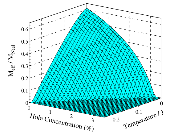
FIG. 1.: Staggered magnetization as function of hole concentration $\delta$ and temperature $T$ for different values of the anisotropy $\epsilon$. $t/J=5,\epsilon=2*10^{-6}$.

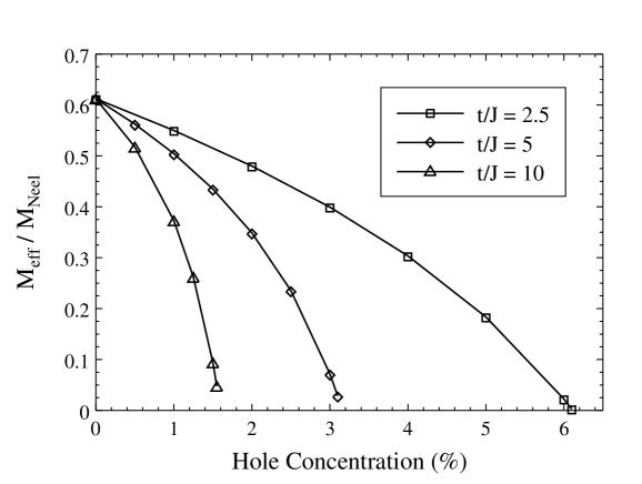
FIG. 2.: Staggered magnetization as function of hole concentration $\delta$ for different values of $t/J$ at zero temperature. The magnetic anisotropy $\epsilon$ is set to zero.

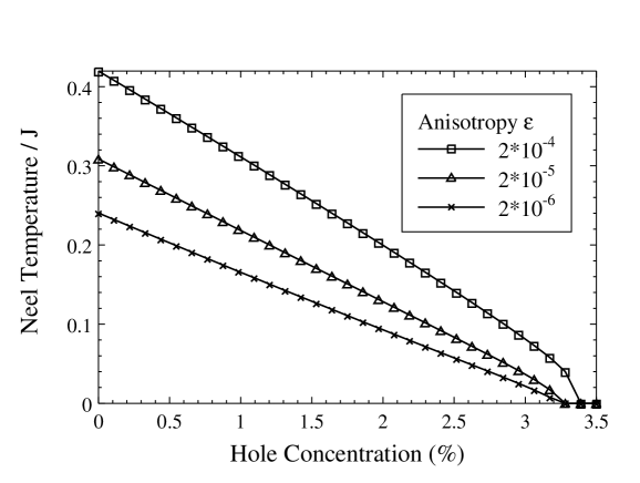
FIG. 3.: Boundary of antiferromagnetic phase for $t/J=5$ and different values of the magnetic anisotropy $\epsilon$. This boundary is given by the condition $M_{eff}=0$.

REFERENCES

• [1] K. W. Becker and P. Fulde, Z. Phys. B 72, 423 (1988)
• [2] K. W. Becker, H. Won, and P. Fulde, Z. Phys. B 75, 335, (1989).
• [3] K. W. Becker and W. Brenig, Z. Phys. B 79, 195 (1990).
• [4] P. Fulde, Electron Correlations in Molecules and Solids.  Berlin: Springer 1993.
• [5] R. Kubo, J. Phys. Soc. Jpn. 17, 1700 (1962).
• [6] G. Polatsek and K. W. Becker, Phys. Rev. B 54, 1637 (1996),
G. Polatsek and K. W. Becker, submitted to Phys. Rev. B (1996).
• [7] H. Köhler and K. W. Becker, Phys. Rev. B 54, ??? (1996).
• [8] T. Schork and P. Fulde, J. Chem. Phys. 97, 9195 (1992).
• [9] K. W. Becker, R. Eder, and H. Won, Phys. Rev. B 45, 4864 (1992).
• [10] M. Vojta and K. W. Becker, Ann. Phys. (Leipzig) 5, 156 (1996).
• [11] M. Vojta and K. W. Becker, Phys. Rev. B 54, 15483 (1996).
• [12] K. Kladko and P. Fulde, preprint MPI-PKS (1996).
• [13] T. Schork and P. Fulde, Int. J. Qu. Chem. 51, 113 (1994).
• [14] P. W. Anderson, Phys. Rev. 86, 694 (1952).
• [15] G. Shirane et $al.$, Phys. Rev. Lett. 59, 1613 (1987).
• [16] J. Rossat-Mignod et $al.$, Physica B 169, 58 (1991).
• [17] E. Dagotto, Rev. Mod. Phys. 66, 763 (1994).
• [18] W. Brenig, Phys. Rep. 251, 153 (1995).
• [19] P. W. Anderson, Science 235, 1196 (1987).
• [20] F. C. Zhang and T. M. Rice, Phys. Rev. B 37, 3759 (1988).
• [21] J. Igarashi and P. Fulde, Phys. Rev. B 45, 12357 (1992).
• [22] G. Khaliullin and P. Horsch, Phys. Rev. B 47, 463 (1993).
• [23] A. Belkasri and J. L. Richard, Phys. Rev. B 50, 12896 (1994).
• [24] J. L. Richard and V. Yu. Yushankhai, Phys. Rev. B 50, 12927 (1994).
• [25] N. D. Mermin and H. Wagner, Phys. Rev. Lett. 17, 1133 (1966).
• [26] C. Bucci et $al.$, Phys. Rev. B 48, 16769 (1993).
• [27] W. F. Brinkman and T. M. Rice, Phys. Rev. B 2, 1324 (1970).
• [28] Y. Nagaoka, Phys. Rev. 147, 392 (1966).
• [29] S. A. Trugman, Phys. Rev. B 37, 1597 (1988).
• [30] B. I. Shraiman and E. D. Siggia, Phys. Rev. Lett. 60, 740 (1988).
• [31] R. F. Bishop, Theor. Chim. Acta 80, 95 (1991).
• [32] R. Kubo, W. E. Brittin, and L. G. Dunham (Eds.), Interscience Publishers Inc., New York 1959.
Refer to caption