An Extended Anderson Model that shows Decreasing Resistivity with Decreasing Temperature

Abstract

The resistivity for an extended two channel Anderson model is calculated. When the temperature decreases, it decreases logarithmically, and has $T^{1/2}$ anomaly at very low temperatures, as seen in some dilute U alloys. The single-particle and the spin excitation spectra are also calculated. The low energy properties and the temperature dependence of the resistivity in the low temperature region are well described by the energy scale deduced from the zero-energy limit of the spin excitation spectrum.

The two channel Kondo model (TCKM) has been studied extensively since Nozières and Blandin pointed out the possibility of the non-Fermi liquid (NFL) behaviours of its ground state [1]. The analytic solutions for the thermodynamic quantities have been obtained by means of the Bethe-Ansatz method [2]. The $\gamma$-coefficient and the susceptibility, $\chi$, diverge as $-$ln$T$ at low temperatures.

Cox has noted that a model for the electronic state of ions with $f^{2}$-configuration, such as ${\rm U^{4+}}$, can be mapped on the TCKM when the crystalline field ground state is the non-Kramers doublet [3]. Many studies have been reported on the applicability of the TCKM to real systems [4-8].

In experiments, a number of dilute U-ion alloys have been known to show the NFL behaviours. Amitsuka and Sakakibara have shown that $\gamma$ and $\chi$ of ${\rm Th_{1-x}U_{x}Ru_{2}Si_{2}}$ have the $-$ln$T$ divergence in the dilute limit. At the same time, the resistivity decreases logarithmically with decreasing temperature, and then decreases in the form $R(0)-c_{R}T^{1/2}$ with negative $c_{R}$ at very low temperatures [9].

Usually $c_{R}$ is expected to be positive for the TCKM. Though Affleck et al. have noted that $c_{R}$ can be negative in the strong exchange cases [10], recent studies based on the numerical renormalization group (NRG) method have shown that the coefficients of the logarithmic divergence of $\gamma$ and $\chi$ are very small for such model [7,11]. Therefore it seems inconsistent with the experimental results.

In a previous paper, we have presented an extended Anderson model which has the possibility of showing the divergent susceptibility and decreasing resistivity with decreasing temperature [12]. The single particle excitation spectrum $\rho_{f}(\omega)$ is given as $\rho_{f}(\omega)\cong\rho_{f}(0)-c_{f}|\omega|^{1/2}$ in the $\omega\rightarrow 0$ limit. The coefficient $c_{f}$ is negative in the weak exchange cases and positive in the strong exchange cases contrasted to the TCKM. Therefore, the resistivity is expected to decrease with decreasing temperature in the weak exchange cases. In this letter, we calculate the temperature dependence of the resistivity for the model, and show that it actually decreases at low temperatures. In addition, we show that the temperature dependence of the resistivity, the spin excitation spectrum, $\rho_{s}(\omega)$, and the single particle excitation spectrum, $\rho_{f}(\omega)$, are well described by one energy scale in the low energy region. The energy scale is extracted from the low energy limit of the spin excitation, $\rho_{s}(0)$.

The extended Anderson model we consider is,

$$H = H_{c}+H_{c-f}+H_{f},$$ (1)

$$H_{f} = \!\sum_{m=(0,\pm 1),\alpha=\pm 1}\!\varepsilon_{fm}n_{m\alpha}$$ (2)

$$+ \frac{U}{2}\sum_{((m=\pm 1)\alpha)\neq((m^{\prime}=\pm 1)\alpha^{\prime})}n_{m\alpha}n_{m^{\prime}\alpha^{\prime}}$$ (3)

$$+ J\!\sum_{(m=\pm 1)\{\alpha\}}\!\vec{\sigma}_{\alpha_{1}\alpha^{{}^{\prime}}_{1}}\vec{\sigma}_{\alpha_{2}\alpha^{{}^{\prime}}_{2}}f_{m\alpha_{1}}^{\dagger}f_{m\alpha^{{}^{\prime}}_{1}}f_{0\alpha_{2}}^{\dagger}f_{0\alpha^{{}^{\prime}}_{2}},$$ (4)

$$H_{c-f} = \sum_{k}\sum_{(m=\pm 1)\alpha}V(f^{\dagger}_{m\alpha}c_{km\alpha}+h.c.),$$ (5)

$$H_{c} = \sum_{k}\sum_{(m=\pm 1)\alpha}\varepsilon_{k}c_{km\alpha}^{\dagger}c_{km\alpha}.$$ (6)

The operator $f_{m\alpha}(c_{km\alpha})$ is the annihilation operator of the localized $f$-electron (conduction electron with wave number $k$). The channel is denoted by $m$, which takes 0 and $\pm 1$, and each has spin freedom, $\alpha=\pm 1$. The quantities $U,J$ and $\varepsilon_{k}$ are the Coulomb interaction constant, the exchange constant and the conduction band energy, respectively. We assume that the band has width from $-D$ to $D$ with $D=1$. The density of states of the conduction electrons, $\rho$, is chosen as constant $\rho=1/2D$. The energy level of the 0-channel, $\varepsilon_{f0}$ is assumed to be deep enough so that $n_{f0}$ is always restricted to 1. In addition, we assume that the energy levels and hybridization matrices of other two channels are independent on $m$, i.e. $\varepsilon_{fm}=\varepsilon_{f}$ and $V_{m}=V$ for $m=\pm 1$. If the orbits of the 0-channel and the $\pm 1$ channels are ascribed, respectively, to the doublet $\Gamma_{7}$ orbit and the quartet $\Gamma_{8}$ orbit in the cubic crystalline field, the present model is similar to the original Anderson model of Cox, from which he derived the TCKM based on the Schrieffer-Wolff transformation and restricting the effective manifold to $f^{2}$-configuration [13].

In this study, we calculate the electric resistivity, $R(T)$, neglecting the vertex correction term. The normalized resistivity is given by

$$R(T)/R(0) = \frac{L_{01}(0)}{L_{01}(T)},$$ (7)

where $L_{ml}$ is defined as

$$L_{ml}(T)=\int^{+\infty}_{-\infty}\left(-\frac{\partial f}{\partial\omega}\right)\omega^{m}\tau(\omega,T)^{l}d\omega.$$ (8)

Here, the relaxation time for the conduction electrons, $\tau(\omega,T)$, is given by using the single particle excitation spectrum of $f$-electron $\rho_{f}(\omega,T)$ as

$$\tau(\omega,T)=\frac{1}{(\pi V^{2}\rho)\rho_{f}(\omega,T)}.$$ (9)

The excitation spectra at finite temperatures are calculated by using the NRG [14,15]. Parameters are chosen mostly to be the same as in our previous paper [12]. The spin excitation spectrum, $\rho_{s}(\omega)$, is defined as the imaginary part of the susceptibility of the operartor, $s^{z}_{f}=\sum_{m=0,\pm 1}s^{z}_{fm}$. The channel excitation spectrum, $\rho_{c}(\omega)$, is that of $n^{c}_{f}=\sum_{m=\pm 1,\alpha=\pm 1}mn_{fm\alpha}$. We define an energy scale, $T^{0}_{\rm K}$, which corresponds to the Kondo temperature of the fictitious two channel Anderson model without the 0-channel spin (FTCAM)[15,16].

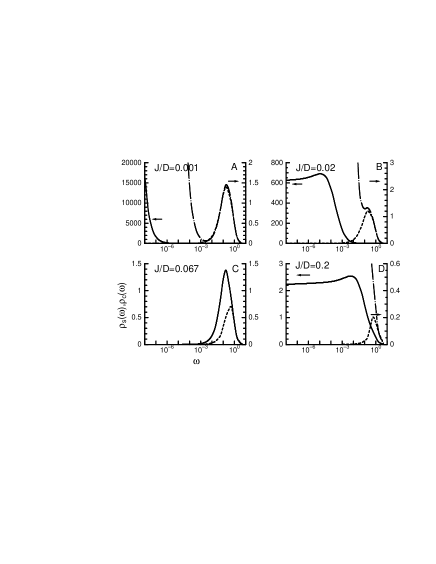
Figure 1: The spin and channel excitation at $T=0$ as a function of the logarithm of the energy, for various $J$. $U=1.0$, $\varepsilon_{f}=-1.5$ and $V^{2}\rho=0.1$. The left ordinate is the scale for the solid line which shows $\rho_{s}(\omega)$. The right ordinate is the scale for the dashed and dot-dashed lines which show $\rho_{s}(\omega)$ and $\rho_{c}(\omega)$ in the magnified scale. The Kondo temperature, $T^{0}_{\rm K}$, for the fictitious two channel Anderson model is estimated to be $\approx$ 0.19. The sign of the coefficient for the $|\omega|^{1/2}$ term in the single particle excitation, $c_{f}$, is negative for A (less than $-10^{4}$) and B($-33$), almost zero for C ($-0.3$), and positive for D ($0.65$).

Figure 1 shows $\rho_{s}(\omega)$ and $\rho_{c}(\omega)$ for various $J$ from the weak exchange cases, $J/T^{0}_{\rm K}<0.35$, to the strong exchange cases, $J/T^{0}_{\rm K}>0.35$. In the weak exchange cases (Figs. 1A and B), $\rho_{s}(\omega)$ has two different structures: one at very low energy and another at about $T^{0}_{\rm K}$. Moreover, $\rho_{s}(\omega)$ has the a finite value in the $\omega\rightarrow 0$ limit, in Fig. 1B. It shows the plateau and decreases steeply at the energy characterized by $0.01/\rho_{s}(0)\sim 10^{-5}$ as $\omega$ increases. The finiteness of $\rho_{s}(0)$ is contrasted to the Fermi liquid behaviour going to zero proportionally to $\omega$ in the $\omega\rightarrow 0$ limit, and it indicates the $-$ln$T$ divergence of the spin susceptibility [17]. As the exchange coupling, $J$, decreases, this NFL structure moves to the lower energy region and $\rho_{s}(0)$ increases (Fig. 1A). In the strong exchange cases (Fig. 1D), $\rho_{s}(0)\times T^{0}_{\rm K}$ seems to be always less than 1.25 [12]. In Fig. 1A, there is a distinct peak at $\omega\sim T^{0}_{\rm K}(=0.19)$. In Fig. 1B, the peak merges into the tail of the NFL structure, and looks like a shoulder. In the weak exchange cases, the height of this peak is much smaller than that of the NFL structure. When $J$ is small enough so that the peak is isolated, it is quite similar to the peak in $\rho_{c}(\omega)$ (Fig. 1A). These peaks in $\rho_{s}(\omega)$ and $\rho_{c}(\omega)$ are formed by the Kondo effect of the FTCAM [16].

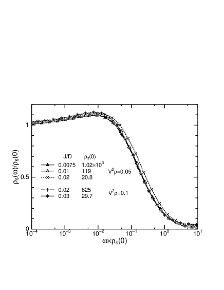
Figure 2: The normalized spin excitation spectra as a function of the normalized energy $\omega\times\rho_{s}(0)$, for various $J$ and $V$. $U=1.0$ and $\varepsilon_{f}=-1.5$, other parameters are shown in the figure. For the all cases, the sign of $c_{f}$ is negative.

In Fig. 2, the normalized spin excitation spectra, $\rho_{s}(\omega)/\rho_{s}(0)$, are shown as a function of $\omega\rho_{s}(0)$. The spectra show good overlapping in the cases of large $\rho_{s}(0)$. When $\rho_{s}(0)$ is large enough so that the NFL structure is well separated from the $\rho_{c}$-like peak at $\omega\sim T^{0}_{\rm K}$, the NFL structure seems to be characterized by one energy scale deduced by $\rho_{s}(0)$.

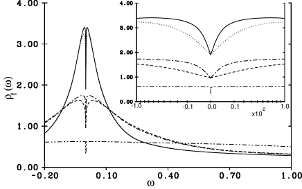
Figure 3: The single particle excitation spectra as a function of energy at $T=0$, for various parameters. The main figure shows the spectrum in the energy range $\approx T^{0}_{\rm K}$. The inset figure shows the cusp structure at around the Fermi energy. The abscissa of the inset is in the square-root of the energy. The parameters are: solid line ($U=1.0$, $J=0.0075$, $V^{2}\rho=0.05$, $T^{0}_{\rm K}=0.11$, $\rho_{s}(0)=1.02\times 10^{3}$), dotted line (1.0, 0.01, 0.05, 0.11, 119), dotted-dashed line (1.0, 0.02, 0.1, 0.19, 625), dashed line (1.0, 0.03, 0.1, 0.19, 29.7), two-dotted-dashed line (0.1, 0.04, 0.3, 1.04, $2.50\times 10^{7}$).

The single particle excitation spectra, $\rho_{f}(\omega)$, at $T=0$ are shown in Fig. 3. When $\omega$ decreases, $\rho_{f}(\omega)$ increases in the energy region $\omega\mathrel{\mathchoice{\lower 4.0pt\vbox{\halign{$\m@th\displaystyle\hfil#\hfil$\cr>\crcr\sim\crcr}}}{\lower 4.0pt\vbox{\halign{$\m@th\textstyle\hfil#\hfil$\cr>\crcr\sim\crcr}}}{\lower 4.0pt\vbox{\halign{$\m@th\scriptstyle\hfil#\hfil$\cr>\crcr\sim\crcr}}}{\lower 4.0pt\vbox{\halign{$\m@th\scriptscriptstyle\hfil#\hfil$\cr>\crcr\sim\crcr}}}}T^{0}_{\rm K}$ almost analogously to the spectrum for the FTCAM. It shows the peaks in both sides of the Fermi energy, and decreases to half of the intensity for the FTCAM as $\omega$ goes to zero [12]. In the very low energy region, $\rho_{f}(\omega)$ has the cusp singularity which is described as $\rho_{f}(\omega)\cong\rho_{f}(0)-c_{f}|\omega|^{1/2}$. As $J$ decreases, the width of the cusp structure becomes narrow.

Figure 4: The normalized single particle excitation as a function of the normalized energy $\omega\rho_{s}(0)$. The main figure shows $\rho_{f}(\omega)$, the abscissa is in the square-root of the energy. The straight fine line represents a fit to $\rho_{f}(\omega)=\rho_{f}(0)-c_{f}|\omega|^{1/2}$. The inset figure shows same quantities in the logarithmic energy scale. The parameters for each lines are same as those in Fig. 3.

Figure 4 shows the normalized single particle excitation, $\rho_{f}(\omega)/\rho_{f}(0)$ at $T=0$, as a function of $\omega\rho_{s}(0)$. The low energy part seems to have a universal shape when we use $1/\rho_{s}(0)$ as the energy unit. In the energy region $\omega<0.1/\rho_{s}(0)$, $\rho_{f}(\omega)$ decreases with decreasing $\omega$ almost linearly with $|\omega|^{1/2}$. Moreover, the universality seems to be valid in the higher energy region where the curves deviate from the simple $|\omega|^{1/2}$ law.

Figure 5: The normalized resistivity as a function of normalized temperature $T\rho_{s}(0)$. The parameters are: solid line ($U=0.1$, $J=0.04$, $V^{2}\rho=0.3$, $\rho_{s}(0)=2.50\times 10^{7}$), dashed line (0.5, 0.10, 0.3, 182), one-dotted-dashed line (0.1, 0.10, 0.3, 53.4), two-dotted-dashed line (1.0, 0.03, 0.1, 29.7). The fine line represents a fit to $R(T)=R(0)-c_{R}T^{1/2}$. The dotted line is the fictitious resistivity which is calculated without the temperature dependence of $\rho_{f}(\omega)$. The parameters are (0.1, 0.04, 0.3, $2.50\times 10^{7}$), same as those of the solid line.

The electric resistivity is shown in Fig. 5. As expected from the numerical results of $\rho_{f}(\omega)$, the resistivity decreases with decreasing temperature. The temperature dependence of the decreasing behaviour is well described by using $1/\rho_{s}(0)$ as the temperature unit. However, we note that the resistivity increases with decreasing temperature at higher temperatures $T\gg T^{0}_{\rm K}$, similarly to the resistivity of the usual Kondo effect. At low temperatures $T<0.05/\rho_{s}(0)$, the resistivity is given as $R(T)\cong R(0)-c_{R}T^{1/2}$, with negative $c_{R}$. Affleck et al. have predicted the relations between the coefficient for the $T^{1/2}$ term and that for the $-$ln$T$ divergent term in thermodynamic quantities for the TCKM [10]. These relations will be checked for the present model in the future paper. In the middle temperature region, $0.05\leq T\rho_{s}(0)\leq 1$, $R(T)$ seems to have the logarithmic temperature dependence.

The fictitious resistivity for which we use $\rho_{f}(\omega,T=0)$ instead of $\rho_{f}(\omega,T)$ in eq. (1) is shown in Fig. 5. Though it is slightly smaller than the proper resistivity, its temperature dependence is not different much from that of the proper resistivity [15].

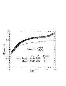
Figure 6: The comparison of the resistivity between our numerical result and the experimental result. The circles show the experimental value for ${\rm Th_{0.97}U_{0.03}Ru_{2}Si_{2}}$. The fitting function is $R_{B}+A(R(T)/R(0))$. The parameter $R_{B}$ is ascribed as the residual resistivity constant of the ${\rm ThRu_{2}Si_{2}}$. The dashed line is given by fitting resistivity at 10K, and the dotted-dashed line is given by supposing $2.6\mu\Omega{\rm cm}$ of the plateau as the unitarity value plus $R_{B}$. In each case, $1/\rho_{s}(0)$ is determined by fitting the $T^{1/2}$ term at very low temperatures.

Figure 6 compares our numerical result of the resistivity with that of ${\rm Th_{1-x}U_{x}Ru_{2}Si_{2}}$ [9]. The calculated result is qualitatively similar to the experimental result. But the ambiguities for determination of the parameters remain [18]. Further study is needed to give a quantitative conclusion [19]. The present model has been by no means directly related to the realistic model of U ion, but the calculation of the model will support the scenario to explain the anomalous properties based on the NFL behaviours of the TCKM type.

In summary, we have calculated the dynamical excitations and the electric resistivity for an extended two channel Anderson model. The leading temperature dependence of the resistivity is proportional to $T^{1/2}$ at very low temperatures. Also there is the temperature region where the resistivity decreases logarithmically. The behaviours are qualitatively similar to the experimental results for ${\rm Th_{1-x}U_{x}Ru_{2}Si_{2}}$. We have shown that the low energy properties are well arranged by one energy scale deduced from the quantity $\rho_{s}(0)$, when the normalized exchange coupling is small, $J/T^{0}_{\rm K}\ll 0.35$. As $J/T^{0}_{\rm K}$ increases, the energy region characterized by the two channel Kondo effect spreads to the higher energy side. The sign changing of $c_{f}$ seems to occur when the spread of the TCKM region becomes comparable to $T^{0}_{\rm K}$.

In this letter, we reported only the symmetric case which the occupation number is $n_{f}=3$ accounting the local spin. Even for the small occupation number cases, $n_{f}<3$, the $T$ dependence of the resistivity at low temperatures is essentially equivalent to that of the symmetric case. Detail will be shown in the future paper.

The authors would like to thank T. Sakakibara, K. Kuwahara, R. Takayama, M. Koga, S. Takagi and H. Suzuki for helpful discussions. The experimental results of the resistivity for ${\rm Th_{1-x}U_{x}Ru_{2}Si_{2}}$ is courtesy by H. Amitsuka. This work was partly supported by Grant-in-Aids No. 06244104, No. 09640451 and No. 09244202 from the Ministry of Education, Science and Culture of Japan. The numerical computation was partly performed at the Computer Center of Institute for Molecular Science (Okazaki National Research Institute), the Computer Center of Tohoku University, and the Supercomputer Center of Institute for Solid State Physics (University of Tokyo).

References

- [1] P. Nozières and A. Blandin : J. Phys. (Paris) 41 (1980) 193.
- [2] P. D. Sacramento and P. Schlottmann : Phys. Rev. B 43 (1990) 295 ; P. B. Wiegmann and A. M. Tsvelick : Pis’ma Zh. Eksp. Teor. Fiz. 38 (1983) 489.
- [3] D. L. Cox Physica B 186-188 (1993) 312.
- [4] Y. Kuramoto, in Transport and Thermal Properties of f-Electron Systems, eds. G. Oomi, H. Fujii and T. Fujita ( Plenum Press, New York, 1993) p.237
- [5] K. Miyake, H. Kusunose and O. Narikiyo : J. Phys. Soc. Jpn. 62 (1993) 2553.
- [6] M. Koga and H. Shiba : J. Phys. Soc. Jpn. 64 (1995) 4345 ; M. Koga and H. Shiba : J. Phys. Soc. Jpn. 65 (1996) 3007.
- [7] H. Kusunose, K. Miyake, Y. Shimizu and O. Sakai : Phys. Rev. Lett. 76 (1996) 271.
- [8] O. Sakai, S. Suzuki and Y. Shimizu : Solid State Commun. 101 (1997) 791.
- [9] H. Amitsuka and T. Sakakibara : J. Phys. Soc. Jpn. 63 (1994) 736 ; T. Sakakibara, H. Amitsuka, D. Sugimoto, H. Mitamura and K. Matsuhira : Physica B 186-188 (1993) 317 ; H. Amitsuka, T. Hidano, T. Honma, H. Mitamura and T. Sakakibara : Physica B 186-188 (1993) 337.
- [10] I. Affleck, A. W. W. Ludwig, H. B. Pang and D. L. Cox : Phys. Rev. B 45 (1992) 7918 ; I. Affleck and A. W. W. Ludwig : Nucl. Phys. B 352 (1991) 849 ; 360 (1991) 641.
- [11] O. Sakai, Y. Shimizu and N. Kaneko : Physica B 186-188 (1993) 322.
- [12] O. Sakai, S. Suzuki, Y. Shimizu, H. Kusunose and K. Miyake : Solid State Commun. 99 (1996) 461.
- [13] We note that the atomic ferromagnetic exchange interaction between -electrons are mapped to the anisotropic antiferromagnetic coupling between and electrons.
- [14] O. Sakai, S. Suzuki, and Y. Shimizu : Physica B 206 & 207 (1995) 141 ; Y. Shimizu and O. Sakai : Computational Physics as a New Frontier in Condensed Matter Research, ed. H. Takayama, M. Tsukada, H. Shiba, F. Yonezawa, M. Imada and Y. Okabe (The Physical Society of Japan, Tokyo, 1995) p. 42.
- [15] S. Suzuki, O. Sakai and Y. Shimizu : J. Phys. Soc. Jpn. 65 (1996) 4034.
- [16] The FTCAM is the Anderson model with four fold degeneracy that the usual Fermi liquid picture is applied. In this model, the channel excitation is equal to the magnetic excitation, and its peak position is good approximation of the usual definition of the Kondo temperature, see reference 15.
- [17] The anomaly is also found in the spin susceptibility which is calculated directly by using the NRG. The numerical results will be published in the near future.
- [18] In the present case, is half of the unitarity limit of the high temperatures. Hence, from the limit () and the high temperature limit () of the experimental resistivity, we can estimate and . The lines in Fig. 6 reaches the unitarity limit at very high temperature . The value at the unitarity limit of the dotted-dashed line is , and that of the dotted line is .
- [19] When we consider a model adding the third extra channel, the resistivity of the low temperatures is expected to decrease more significantly because the phase shift of the third channel tends to zero in the low energy limit. (see Y. Shimizu, O. Sakai and S. Suzuki in proceedings of ICM ’97). This modified case will show the resistivity that is more similar to the experimental results.