The Weak Localization Correction to the Polarization and Persistent Currents in Mesoscopic Metal Rings

Abstract

We re-examine the effect of electron-electron interactions on the persistent current in mesoscopic metal rings threaded by an Aharonov-Bohm flux. The exchange contribution to the current is shown to be determined by the weak localization correction to the polarization. We explicitly calculate the contribution from exchange interactions with momentum transfers smaller than the inverse elastic mean free path to the average current, and find that it has the same order of magnitude as the canonical current without interactions.
Keywords: weak localization, persistent currents

PACS numbers: 73.50.Bk, 72.10.Bg, 72.15.Rn

The persistent current in mesoscopic metal rings threaded by a static magnetic flux $\phi$ is a striking manifestation of the quantum nature of charge transport in phase-coherent systems[1, 2]. At the first sight one might expect that this effect can be explained within a model of non-interacting electrons in a random potential. Surprisingly, the seminal experiment by Lévy et al.[3] revealed that in the diffusive regime the average current is more than two orders of magnitude larger than the theoretically predicted current for non-interacting electrons[4]. Therefore it seems inevitable to invoke electron-electron interactions to explain the experiment[3]. This was first attempted by Ambegaokar and Eckern (AE)[5], who calculated perturbatively the correction to the average current to first order in the screened Coulomb interaction. They found an average current proportional to $\lambda_{\rm cb}{ev_{F}}\ell/{L}^{2}$, where $\lambda_{\rm cb}$ is a dimensionless measure for some suitably averaged strength of the Coulomb interaction at short wavelengths, $v_{F}$ is the Fermi velocity, $\ell$ is the elastic mean free path, and $L$ is the circumference of the ring. The precise value of $\lambda_{\rm cb}$ is difficult to estimate, because it is dominated by the non-universal short-wavelength part of the Coulomb interaction. Using [6] $\lambda_{\rm cb}\approx 0.06$, the theoretical current is still a factor of $5$ too small to explain the experiment.

More recently one of us has argued that the classical (Hartree) contribution to the persistent current is strongly enhanced due to the long-range nature of the bare Coulomb interaction[7]. Although the arguments put forward in Ref.[7] have been criticized[8], we believe that the criticism did not properly take the essentially non-perturbative nature of these arguments into account[9]. However, this is not the subject of this note.

Here we would like to re-examine the exchange (Fock) contribution to the average current. It is well known[10] that for disordered metals singular vertex corrections involving so-called diffusons strongly enhance the effective exchange interaction at small wave-vectors $|{\bf{q}}|\raisebox{-2.15277pt}{$\;\stackrel{{\scriptstyle<}}{{\sim}}\;$}2\pi/\ell$. This effect has been ignored by AE[5], who focused on the short-wavelength part of the interaction. The possible relevance of these diffusive vertex corrections for persistent currents has been pointed out some time ago by Béal-Monod and Montambaux[11]. However, they also demonstrated that there exists an overall cancellation of the leading infrared singularities. Up until now a quantitative calculation of the persistent current due to exchange interactions with small momentum transfers has not been performed. In this work we shall present a simple solution of this problem.

It is instructive to obtain the (grand canonical) persistent current $I=-c\partial\Omega(\phi)/\partial\phi$ from the Grassmannian functional integral representation of the ratio ${\cal{Z}}/{\cal{Z}}_{0}=e^{-(\Omega-\Omega_{0})/T}$ of the partition functions with and without interactions. Here $T$ is the temperature. Decoupling the Coulomb interaction by means of a Hubbard-Stratonovich field $V$ and integrating over the Grassmann fields, we obtain after the usual transformations[12] ${\cal{Z}}/{\cal{Z}}_{0}=\int{\cal{D}}\{V\}e^{-S_{\rm eff}\{V\}}$, with the effective action[13]

$$S_{\rm eff}\{V\}=\frac{T}{2}\sum_{q}f^{-1}_{\bf{q}}V_{-q}V_{q}-2{\rm Tr}\ln\left[1-\hat{G}_{0}\hat{V}\right]\;,$$ (1)

where the factor of $2$ in front of the trace is due to the spin degeneracy, and $f_{\bf{q}}$ is the Fourier transform of the Coulomb potential[14]. $\hat{V}$ and $\hat{G}_{0}$ are infinite matrices in frequency and wave-vector space, with matrix elements $[\hat{V}]_{kk^{\prime}}=iTV_{k-k^{\prime}}$ and[13]

$$[\hat{G}_{0}^{-1}]_{kk^{\prime}}=\delta_{kk^{\prime}}[i\tilde{\omega}_{n}-\xi_{\bf{k}}]-\delta_{nn^{\prime}}U_{{\bf{k}}-{\bf{k}}^{\prime}}\;.$$ (2)

Here $U_{\bf{q}}$ is the Fourier transform of the disorder potential (assumed to be Gaussian white noise), and $\xi_{\bf{k}}={\bf{k}}^{2}/(2m)-\mu$, where $m$ is the (effective) mass of the electrons, and $\mu$ is the chemical potential. Identifying the position along the circumference of the ring with the $x$-coordinate, the flux-dependence of $\Omega(\phi)$ is due to the quantization $k_{x}=\frac{2\pi}{L}(n+\phi/\phi_{0})$, $n=0,\pm 1,\ldots$ of the $x$-component of the wave-vector.

For a calculation to first order in the RPA (random phase approximation) screened interaction it is sufficient to expand the logarithm in Eq.(1) to second order,

$$S_{\rm eff}\{V\} \approx i\sum_{{q}}N_{0}(q)V_{-{q}}$$ (4)

$$+\frac{T}{2}\sum_{qq^{\prime}}\left[\delta_{qq^{\prime}}f^{-1}_{\bf{q}}+\Pi_{0}(q,q^{\prime})\right]V_{-q}V_{q^{\prime}}+\ldots\;\;,$$

where $N_{0}({{q}})=2T\sum_{k}[\hat{G}_{0}]_{k+q,k}$ and

$$\Pi_{0}(q,q^{\prime})=-2T\sum_{kk^{\prime}}[\hat{G}_{0}]_{k+q,k^{\prime}+q^{\prime}}[\hat{G}_{0}]_{k^{\prime}k}\;.$$ (5)

Note that $[\hat{G}_{0}]_{kk^{\prime}}$ in Eq.(2) is proportional to $\delta_{nn^{\prime}}$, so that $N_{0}(q)=\delta_{n0}N_{0}({\bf{q}})$ can be identified with the spatial Fourier component of the density for a given realization of the disorder, and $\Pi_{0}(q,q^{\prime})=\delta_{nn^{\prime}}\Pi_{0}({\bf{q}},{\bf{q}}^{\prime},i\omega_{n})$ is the non-interacting polarization. The linear term in Eq.(4) can be eliminated by means of the shift-transformation $V_{q}\rightarrow V_{q}-iT^{-1}\sum_{q^{\prime}}f^{\rm RPA}_{qq^{\prime}}N_{0}(q^{\prime})$, where $f^{\rm RPA}_{qq^{\prime}}$ is the inverse of the infinite matrix with elements $\delta_{qq^{\prime}}f^{-1}_{\bf{q}}+\Pi_{0}(q,q^{\prime})$. To calculate the persistent current it is convenient to take the derivative of $\ln({\cal{Z}}/{\cal{Z}}_{0})$ with respect to $\phi$ before performing the Gaussian integration over the auxiliary field $V$. In this way we obtain $I=I_{0}+I_{H}+I_{F}$, where $I_{0}$ is the non-interacting persistent current, and

$$I_{H} = \frac{-c}{2}\frac{\partial}{\partial\phi}\sum_{{\bf{q}}{\bf{q}}^{\prime}}f^{\rm RPA}_{{\bf{q}}{\bf{q}}^{\prime}}N_{0}(-{\bf{q}})N_{0}({\bf{q}}^{\prime})\;,$$ (6)

$$I_{F} = \frac{-c}{2}\sum_{{\bf{q}}{\bf{q}}^{\prime}}T\sum_{n}f^{\rm RPA}_{{\bf{q}}i\omega_{n},{\bf{q}}^{\prime}i{\omega}_{n}}\frac{\partial}{\partial\phi}\Pi_{0}({\bf{q}},{\bf{q}}^{\prime},i\omega_{n})\;.$$ (7)

Note that the Hartree contribution $I_{H}$ involves only the static part $f^{\rm RPA}_{{\bf{q}}{\bf{q}}^{\prime}}\equiv f^{\rm RPA}_{{\bf{q}}0,{\bf{q}}^{\prime}0}$ of the screened interaction.

Let us now focus on the average Fock current $\overline{I}_{F}$ in the diffusive regime, where the over-bar denotes the disorder average. To leading order in the small parameter $(k_{F}\ell)^{-1}$ (where $k_{F}$ is the Fermi wave-vector) we may factorize the average, so that we need to know the flux-derivative of the average polarization $\partial\overline{\Pi}_{0}({\bf{q}},i\omega)/\partial\phi$. Note that after averaging the polarization is diagonal in wave-vector space. It is easy to show[15] that the result of AE[5] can be reproduced if one retains only diagram (a) in Fig.1. For $|{\bf{q}}|\ll k_{F}$ and $|\omega|\tau\ll 1$ (where $\tau=\ell/v_{F}$ is the elastic lifetime) this diagram yields

$$\frac{\partial}{\partial\phi}\overline{\Pi}_{0}({\bf{q}},i\omega)_{\rm AE}=\Delta^{-1}{|\omega|\tau}\frac{\partial}{\partial\phi}g_{\rm WL}(i\omega,\phi)\;,$$ (8)

where $\Delta$ is the average level-spacing at the Fermi energy. $g_{\rm WL}(i\omega,\phi)$ is the well known weak-localization correction to the dimensionless average conductivity $\overline{\sigma}(i\omega)$ in units of the corresponding Drude conductivity $\sigma_{0}$,

$$\overline{\sigma}(i\omega)=\sigma_{0}[1+g_{\rm WL}(i\omega,\phi)]\;,$$ (9)

$$g_{\rm WL}(i\omega,\phi)=-\frac{2\Delta}{\pi}{\sum_{{\bf{Q}}}}^{\prime}\frac{1}{{\cal{D}}_{0}{\bf{Q}}^{2}+|{\omega}|+{\cal{D}}_{0}/L_{\varphi}^{2}}\;,$$ (10)

where ${\cal{D}}_{0}=v_{F}\ell/3$ is the classical diffusion coefficient. Note that ${\cal{D}}_{0}$ and $\sigma_{0}$ are related via the classical Einstein relation $\sigma_{0}=(\Delta{\cal{V}})^{-1}e^{2}\sigma_{0}$, where ${\cal{V}}$ is the volume of the system. The prime in Eq.(10) means that the sum is restricted to $|{\bf{Q}}|\raisebox{-2.15277pt}{$\;\stackrel{{\scriptstyle<}}{{\sim}}\;$}2\pi/\ell$. Here the $x$-component of ${\bf{Q}}$ is quantized according to ${Q}_{x}=\frac{2\pi}{L}(n+2\phi/\phi_{0})$, and $L_{\varphi}$ is the dephasing length[10].

Clearly, the approximation (8) cannot be correct for $|{\bf{q}}|\ell\ll 1$, because then the density vertices in Fig.1(a) can be dressed by singular diffuson corrections, as shown in Figs.1(b)–(d). As a consequence, this regime requires a special treatment. This has already been noticed by Béal-Monod and Montambaux[11]. Unfortunately, the sum of diagrams (b)–(d) in Fig.1 cancels to leading order in $(k_{F}\ell)^{-1}$[11], so that at the first sight it seems that the calculation of the leading non-vanishing behavior of $\partial\overline{\Pi}_{0}({\bf{q}},i\omega)/\partial\phi$ requires rather complicated mathematical manipulations. However, there is a simple way to avoid this technical complication: As shown in Ref.[16], current conservation implies that for small wave-vectors and frequencies the polarization is of the form

$$\overline{\Pi}_{0}({\bf{q}},i\omega)=\Delta^{-1}\frac{{\cal{D}}(i\omega){\bf{q}}^{2}}{{\cal{D}}(i\omega){\bf{q}}^{2}+|\omega|}\;,$$ (11)

where ${\cal{D}}(i\omega)$ is the generalized frequency-dependent diffusion coefficient, which is related to the frequency-dependent average conductivity $\overline{\sigma}(i\omega)$ via[16]

$$\frac{{\cal{D}}(i\omega)}{{\cal{D}}_{0}}=\frac{\overline{\sigma}(i\omega)}{\sigma_{0}}\;.$$ (12)

Combining Eq.(12) with Eqs.(9) and (10), we conclude

$$\frac{\partial}{\partial\phi}{\cal{D}}(i\omega)={\cal{D}}_{0}\frac{\partial}{\partial\phi}g_{\rm WL}(i\omega,\phi)\;.$$ (13)

From Eqs.(11) and (13) it is now obvious that the flux-dependence of the average polarization can be expressed in terms of the weak localization correction (10) to the dynamic conductivity. After a straightforward calculation we finally obtain

$$\frac{\partial}{\partial\phi}\overline{\Pi}_{0}({\bf{q}},i\omega) = \Delta^{-1}\frac{|\omega|{\cal{D}}_{0}{\bf{q}}^{2}}{\left[{\cal{D}}_{0}{\bf{q}}^{2}[1+g_{\rm WL}(i\omega,\phi)]+|\omega|\right]^{2}}$$ (14)

$$\times \frac{\partial}{\partial\phi}g_{\rm WL}(i\omega,\phi)\;.$$ (15)

This expression, which is one of the main results of this work, is valid in the regime $|{\bf{q}}|\raisebox{-2.15277pt}{$\;\stackrel{{\scriptstyle<}}{{\sim}}\;$}2\pi/\ell$ and $\Delta\ll|\omega|\raisebox{-2.15277pt}{$\;\stackrel{{\scriptstyle<}}{{\sim}}\;$}\tau^{-1}$. For $|\omega|\raisebox{-2.15277pt}{$\;\stackrel{{\scriptstyle<}}{{\sim}}\;$}\Delta$ more sophisticated methods are necessary to obtain the weak localization correction to the polarization[17]. For our purpose Eq.(15) is sufficient, because the average of Eq.(7) is dominated by frequencies in the range $\Delta\ll|\omega|\raisebox{-2.15277pt}{$\;\stackrel{{\scriptstyle<}}{{\sim}}\;$}E_{c}$, where $E_{c}={\cal{D}}_{0}/L^{2}$ is the Thouless energy. Note that for $|{\bf{q}}|\ell=O(1)$ Eq.(15) smoothly matches the short wavelength result (8). In fact, using ${\cal{D}}_{0}=v_{F}\ell/3$, we see that for $|g_{\rm WL}|\ll 1$ both expressions are identical at $|{\bf{q}}|\ell=\sqrt{3}$. On the other hand, in the regime $|{\bf{q}}|\ell\ll 1$ the long-wavelength result (15) is a factor of $({\bf{q}}\ell)^{-2}$ larger than Eq.(8).

To see whether this infrared enhancement is sufficient to lead to a significant exchange contribution to the persistent current, we substitute Eq.(15) into Eq.(7). Then we obtain for the long-wavelength Fock contribution to the average current

$$\overline{I}_{F}^{\rm long} = -\frac{c}{2}T\sum_{n}{\sum_{\bf{q}}}^{\prime}\frac{f_{\bf{q}}\frac{\partial}{\partial\phi}\overline{\Pi}_{0}({\bf{q}},i\omega_{n})}{1+f_{\bf{q}}\overline{\Pi}_{0}({\bf{q}},i\omega_{n})}$$ (16)

$$\approx -\frac{c}{2}T\sum_{n}\left[{\sum_{\bf{q}}}^{\prime}\frac{|\omega_{n}|}{{\cal{D}}_{0}{\bf{q}}^{2}[1+g_{\rm WL}(i\omega_{n},\phi)]+|\omega_{n}|}\right]$$ (18)

$$\times\frac{\frac{\partial}{\partial\phi}g_{\rm WL}(i\omega_{n},\phi)}{1+g_{\rm WL}(i\omega_{n},\phi)}\;,$$

where the second line is valid in the experimentally relevant limit $|f_{\bf{q}}\overline{\Pi}_{0}({\bf{q}},i\omega_{n})|\gg 1$. Note that the current (18) increases with the strength of the disorder, because the (negative) weak-localization correction $g_{\rm WL}$ in the denominator of Eq.(18) becomes more and more important with increasing disorder, thus reducing the screening. Of course, our calculation is only controlled for $|g_{\rm WL}|\ll 1$, so that from now on this correction will be ignored. For simplicity let us assume that the ring is sufficiently thin, such that only the motion along the circumference is diffusive. In this case the ${\bf{q}}$-sum in the square brace of Eq.(18) can be replaced by a one-dimensional integral, which for $L\gg\ell$ is independent of the ultraviolet cutoff. We obtain

$$\overline{I}_{F}^{\rm long}=-\frac{c}{4}T\sum_{n}\left[\frac{|\omega_{n}|L^{2}}{{\cal{D}}_{0}}\right]^{1/2}\frac{\partial}{\partial\phi}g_{\rm WL}(i\omega_{n},\phi)\;.$$ (19)

For $T\rightarrow 0$ and $L_{\varphi}\gg L$ the summation over the Matsubara frequencies can be performed exactly, and we finally arrive at

$$\overline{I}_{F}^{\rm long}=-\frac{ev_{F}}{L}\frac{\pi}{(k_{F}L_{\bot})^{2}}f(\phi)\;,$$ (20)

where $L_{\bot}$ is the transverse thickness of the ring, and

$$f(\phi) = \frac{2}{\pi}\sum_{m=1}^{\infty}\frac{\sin(4\pi m\phi/\phi_{0})}{m}$$ (21)

$$= 1-4\phi/\phi_{0}\;\;\;,\;\;\;\mbox{for $0<\phi/\phi_{0}<1/2$}\;.$$ (22)

Surprisingly, this current has the same order of magnitude as the non-interacting current at constant particle number[4]. In the experimentally relevant parameter regime[3], this current is smaller than the current due to the short wavelength part of the Coulomb interaction calculated by AE[5].

In summary, we have presented a quantitative calculation of the long-wavelength exchange contribution to the average persistent current in mesoscopic metal rings. The current has the same order of magnitude as the non-interacting persistent current at constant particle number. We have also calculated the leading weak localization correction to the average polarization $\overline{\Pi}_{0}({\bf{q}},\omega)$ in the regime $|{\bf{q}}|\raisebox{-2.15277pt}{$\;\stackrel{{\scriptstyle<}}{{\sim}}\;$}2\pi/\ell$ and $\Delta\raisebox{-2.15277pt}{$\;\stackrel{{\scriptstyle<}}{{\sim}}\;$}|\omega|\ll\tau^{-1}$, effectively taking singular diffuson corrections to the density vertices into account.

This work was supported by the Deutsche Forschungsgemeinschaft (SFB 345), and by the ISI Foundation (ESPRIT 8050 Small Structures). The work of PK was partially carried out at the Villa Gualino, Torino.

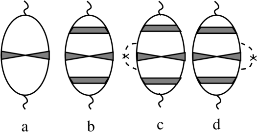
FIG. 1.: Diagrams contributing to $\partial\overline{\Pi}_{0}({\bf{q}},i\omega)/\partial\phi$. Retaining only (a) reproduces the result of AE. The shaded triangles represent the Cooperon, the solid lines are average non-interacting Green’s functions, and the small wavy lines denote density vertices. (b) Vertex correction with two additional diffusons (represented by shaded stripes). For small ${\bf{q}}$ and $\omega$ this diagram is much larger than (a). However, to leading order in $(k_{F}\ell)^{-1}$ (b) is cancelled by (c) and (d). Here the dashed lines denote the impurity average $\overline{U_{\bf{q}}U_{\bf{-q}}}$.

REFERENCES

- [1] F. Hund, Ann. Phys. (Leipzig) 32, 102 (1938).
- [2] M. Büttiker, Y. Imry, and R. Landauer, Phys. Lett. 96 A, 365 (1983).
- [3] L. P. Lévy et al., Phys. Rev. Lett. 64, 2074 (1990).
- [4] A. Schmid, Phys. Rev. Lett. 66, 80 (1991); F. von Oppen and E. K. Riedel, Phys. Rev. Lett. 66, 84 (1991). B. L. Altshuler, Y. Gefen, and Y. Imry, Phys. Rev. Lett. 66, 88 (1991).
- [5] V. Ambegaokar and U. Eckern, Phys. Rev. Lett. 65, 381 (1990); ibid. 67, 3192 (1991).
- [6] U. Eckern, Z. Phys. B 82, 393 (1991).
- [7] P. Kopietz, Phys. Rev. Lett. 70, 3123 (1993); 71, 306, (1993) (E).
- [8] G. Vignale, Phys. Rev. Lett. 72, 433 (1994); A. Altland and Y. Gefen, ibid. 2973 (1994).
- [9] P. Kopietz, Phys. Rev. Lett. 72, 434 and 2974 (1994). Note that the arguments of Ref.[8] are based on the naive expansion (6) in powers of the RPA interaction, rather than on the self-consistent Hartee current. We therefore would like to maintain that Ref.[7] is essentially correct, although we have not been able to provide a complete microscopic justification within diagrammatic perturbation theory. As explained in A. Völker and P. Kopietz, Z. Phys. B 100, 545 (1997), the calculation in Ref.[7] implicitly relies on the fact that in disordered mesoscopic metals well-defined quasi-particles exist only in a small energy window close to the Fermi energy, see U. Sivan, Y. Imry and A. G. Aronov, Europhys. Lett. 28, 115 (1994).
- [10] See, for example, the articles by B. L. Altshuler and A. G. Aronov, or by H. Fukuyama in: Electron-Electron Interactions in Disordered Systems, edited by A. L. Efros and M. Pollak (North Holland, Amsterdam, 1985).
- [11] M. T. Béal-Monod and G. Montambaux, Phys. Rev. B 46, 7182 (1992).
- [12] See, for example, chapter 3 of P. Kopietz, Bosonization of Interacting Fermions in Arbitrary Dimensions, (Lecture Notes in Physics m48, Springer, Berlin, 1997).
- [13] We use the notation and , where are bosonic and are fermionic Matsubara frequencies.
- [14] In a finite system the Fourier transform of the Coulomb potential does not have any singularities. It is then convenient to normalize in Eq.(1) such that for , where is the classical capacitance[7]. Similarly, the polarization is normalized such that to leading order .
- [15] A. Völker and P. Kopietz, (unpublished).
- [16] D. Vollhardt and P. Wölfle, Phys. Rev. B 22, 4666 (1980).
- [17] K. B. Efetov, Phys. Rev. Lett. 76, 1908 (1996); Ya. M. Blanter and A. B. Mirlin, Phys. Rev. B 53, 12601 (1996); preprint cond-mat/9705250.