Local state space geometry and thermal relaxation in complex landscapes: the spin-glass case.

Abstract

A simple geometrical characterization of configuration space neighborhoods of local energy minima in spin glass landscapes is found by exhaustive search. Combined with previous Monte Carlo investigations of thermal domain growth, it allows a discussion of the connection between real and configuration space descriptions of low temperature relaxational dynamics. We argue that the part of state-space corresponding to a single growing domain is adequately modeled by a hierarchically organized set of states and that thermal (meta)stability in spin glasses is related to the nearly exponential local density of states present within each trap.

I Introduction

In this paper we consider the relation between configuration space geometry, excitation morphology and relaxation dynamics of spin glass systems. Spin glasses have a complex landscape fraught with local (free) energy minima, which, at sufficiently low temperatures, prevent the system from reaching a state of global thermal equilibrium: slow relaxation becomes the dominating observable features of the system on relevant time scales, and thus a main point of theoretical interest. Despite the absence of global equilibration, spin glasses – as well as other complex systems displaying broken ergodicity[1]– relax through a series of quasiequilibria involving subsets of configuration space (traps or metastable regions). Hence, during relevant experimental time windows measurable quantities appear as canonical averages restricted to the configurations of the trap, and the latter can be considered as a single point in the free energy landscape of the system. Free energy barriers separating metastable regions can be probed by so called aging experiments[2, 3]: In Zero Field Cooled (ZFC) experiments[4], the system is rapidly cooled in zero field to a temperature $T_{m}$ and is then left undisturbed for a time $t_{w}$. Thereafter, a small magnetic field is turned on, and the growing magnetic response of the system is measured. In Thermo Remanent Magnetization (TRM) experiments[5] the system is quickly cooled to $T_{m}$ and allowed to relax in a magnetic field for a time $t_{w}$. The field is then cut and the decay of the magnetization is measured. In both cases the response curve strongly depends on the time $t_{w}$ elapsed previous to the field change. Qualitatively, this can be understood by the idea of partial equilibration just explained: after relaxing for a time $t_{w}$ the system occupies a valley in state space with a characteristic size related to $t_{w}$. Probing the system on times scales less than $t_{w}$ reveals properties of the equilibrium fluctuations in this valley, while probing on longer time scales gives the non-equilibrium properties[6]. Numerically, a coarse grained picture of configuration space relaxation can be obtained directly for microscopic systems of modest size [7, 8] by constructing the connectivity matrix of a subset of state space and solving the master equation for the probability flow. For each time, configurations mutually close to equilibrium are lumped together, yielding a relaxation tree which describes the merging in time of larger and larger subset of internally equilibrated states.

Theories of spin glass dynamics are either based on assumed scaling properties of low energy excitations in real space[9, 10, 11], or on mesoscopic hierarchical models of state space, reviewed for instance in Ref.[12]. Some of the approaches in the latter category are inspired by the equilibrium properties of mean field models[13], whose relevance for short-range spin glasses is now hotly debated[14]. However, hierarchical models can also simply be viewed [15] as paradigms of sequential, strongly constrained dynamics, without reference to any equilibrium property. The models generally feature a sequence of increasing barriers, delimiting larger and larger subsets of state space. The simplest class of mathematically analyzable structures with this property are trees. Master equations on trees[19, 20, 21, 22, 23, 24, 25] have propagators which decay algebraically in time, and a decay exponent (or exponents[24]) with a linear or s-shaped temperature dependence ( depending on the particular model ). When simple ‘magnetic’ assumptions are introduced, one can reproduce the AC susceptibility curves [26], the aging behavior[27, 28, 29], including changes of the apparent age due to a temperature step[30] and age reset by temperature cycling[31]. As the predictions of hierarchical models are in good agreement with the experimental facts, a direct check of their basic assumptions seems a worthwhile endeavor. We note that as low temperature excitations in spin-glasses are small non-interacting clusters in a frozen environment[16, 17, 18], parallel and sequential modes of relaxation must both be represented in the dynamics. This leads to the question of exactly what parts of state space, if any, hierarchical models describe, and to the allied, more general question, of the relation between state space phenomenologies and the widely used domain growth approaches.

A numerical state space analysis is attempted here, by exhaustively enumerating and statistically analyzing millions to hundreds of millions of configurations close to deep energy minima. We do not try to study the state-space dynamics directly, since the problem sizes considered prevent us from calculating connectivity matrices and numerical solving the master equation for thermalization. Exhaustive search is insensitive to entropic barriers[32] and gives therefore incomplete information with regard to dynamical properties. However, by including in the discussion previous studies of domain growth and by using simple heuristic arguments, some conclusions can be drawn about thermal (meta)stability.

The extensive calculations required in this investigation were done on a Silicon Graphics Onyx parallel machine with 24 processors and 2 gigabytes of RAM at the University of Odense, Denmark, and on a Silicon Graphics 32 CPU Origin2000 with up to 32 GB of RAM kindly made available to this project by the SGI Advanced Technology Centre in Cortaillod, Switzerland.

II Method and results

Low temperature excitations in spin glasses are small connected domains of spins which are reversed relative to the their orientation in a very low energy configuration. This gives rise to a block structure in state space, where each block contains the dynamically available states of a single domain. Insight in the state-space geometry of one block can arguably be obtained by considering systems of size comparable to a domain: At low $T$ this typically means up to $10^{d}$ spins, where $d$ is the dimension. Even in such relatively small systems the number of configurations quickly becomes astronomical, precluding the possibility of examining all the configurations. Instead, one can use the ‘lid method’, which exhaustively visits relevant low-energy parts of the landscape. [7, 8]. A brief outline of the method is given here for completeness, while a more technical description, including details of the algorithm parallel implementation and performance statistics, is planned for a separate publication[33].

Consider a nearest neighbor walk which starts at a local energy minimum, or reference state, $\psi$, which, by definition, has zero energy. All states with energy above an energy ‘barrier’, $L$ are excluded from the walk. We let ${\cal P}_{\psi,L}$ be the set of all states which can be visited in such a walk. Following our previous notation[7] we refer to ${\cal P}_{\psi,L}$ as a pocket of depth $L$ centered at $\psi$. As, in a thermal relaxation process, the ‘typical’ time needed to exit ${\cal P}_{\psi,L}$ (whether it be a first passage time or an average ) contains the factor $\exp(L/T)$, which is large at low temperatures, ${\cal P}$ is a bona fide candidate for a metastable region operationally defined by an energy barrier.

The reference state $\psi$ is constructed by an iterative process. Initially, we pick a random state ${\cal\psi}_{0}$ to start the exhaustive search. As soon as a new state with lower energy $\psi_{1}$ is found, it becomes the current reference states and it is used as a starting point of a new search. At the $n^{\prime}th$ stage of the process $\psi_{n}$ is the state of current lowest energy among all states examined. In this way the search algorithm ‘digs’ deeper and deeper into the landscape. The program stops when a certain fraction of the spins in the system (usually one half) is flipped without finding any state with energy lower than the current reference state. The latter is becomes then, by definition, the ‘deep’ minimum $\psi$. Our exhaustive approach considerably differs from that of Vertechi and Virasoro[34], who sampled the distribution of energy barriers separating zero temperature solutions of the TAP equation: in our case the barrier is a parameter defining the pocket and all states in the pocket are found deterministically, allowing the calculation of the local density of states.

The spin glass problem deals with a set of $\cal N$ Ising spins $\sigma_{i}={\scriptstyle\stackrel{{\scriptstyle+}}{{-}}}1$ placed on a 2D or 3D cubic lattice with periodic boundary conditions. The energy of the $x$’th configuration, $0<x\leq 2^{\cal N}$, is defined by the well known Hamiltonian[35]

$$E(x)=-\frac{1}{2}\sum_{i,j}J_{ij}\sigma_{i}(x)\sigma_{j}(x),$$ (1)

where $J_{ij}=J_{ji}$ and where $J_{ij}\neq 0$ only if spins $i$ and $j$ are adjacent on the grid. In this case, and for $i<j$,  we take the $J_{ij}$’s as independent gaussian variables, with zero average and variance $J^{2}=1$. By definition neighbor configurations are those which differ by the orientation of exactly one spin.

Data are analyzed with an eye to the properties of mesoscopic state-space models. First and foremost we investigate, for $E\leq L$, the energy distribution of the states or local density of states ${\cal D}(E,L)$ within a pocket of depth $L$. The integral of this quantity over its first argument is the state-space volume of the pocket, ${\cal V}(L)$. In most cases, the reference state $\psi$ has the property that half of its spins can be overturned without finding any state of lower energy. Let $L_{1/2}$ be the corresponding energy barrier. For the smallest examples considered this barrier was found (within a small tolerance) to also allow the system to reach the spin reversed state $-\psi$[36]. By chosing different initial condition for the search, while keeping the $J_{ij}$ fixed, different deep reference minima can be found which are unrelated by global flips and which all have energies per spin at or below estimates of the ground state energy of spin-glasses[37]. We also present data for more shallow pockets, i.e. where the reference state is not particularly low-lying. We furthermore calculate the barrier values for which the current largest Hamming distance to the reference state increases its value, and the average number of neighbors to which a state is connected as a function of the lid. This number would be constant and equal to the number of spins if all neighbors were available, but as high lying states are discarded, the effective connectivity is much lower.

All the investigations are performed for two and three dimensional lattices, which have similar patterns of low temperature relaxation[38]. In both dimensions we analyze, for a series of lattice sizes, $25$ different realizations of the $J_{ij}$’s. As usual, disorder averages are performed. Furthermore we try to convey an idea of the system to system and pocket to pocket variation. In all cases we attempted to perform the exhaustive search up to the barrier value $L_{1/2}$. Due to memory limitations, this was unfortunately not always possible for the largest among the systems considered: For the $10^{2}$ systems we succeeded in 24 cases out of 25, missing by two spins in the unsuccessful case, while for the $6^{3}$ systems we succeeded in $20$ cases out of $25$. The remaining instances had to be stopped at different stages of the calculation. The value of $L_{1/2}$ and the size of the corresponding pockets greatly vary from sample to sample. For ease of display, we used the total volume of each pocket as a normalization factor for the corresponding local density of states. This creates vertical shifts of the data which are void of physical significance.

Before considering any issue of interpretation, it is interesting to note that all the data can be parametrized rather simply: the local density of states is almost exponential, with a small systematic downward curvature (see Figs. 1-4). The available volume in the pocket is also close to an exponential function of the lid energy, if one smooths out the jumps which occur when a new ‘side pocket’ appears as the barrier increases (see Figs. 7 and 8). Finally, the largest obtainable Hamming distance to the reference state grows exponentially with the barrier defining the pocket(see Figs. 5-6). All these properties are common to deep and less deep pockets.

The exponential form of the local density of states is shown directly in Figs. 1 and 2 for $10^{2}$ and $5^{3}$ systems respectively. In these plots the raw data are indicated by different symbols, one for each realization of the couplings, while the lines are calculated by fitting $\log({\cal D}(E,L_{max}))$ to a parabola in $E$. The coefficient of the second order term is typically 20 times smaller than the coefficient of the linear term in 2D, and 50 times smaller in 3D. Therefore, the reciprocal of the linear coefficient basically describes the energy scale of the exponential density of state at low energies. These coefficients are plotted versus the system size in Figs. 3 and 4 for a number of 2D and 3D systems respectively. As discussed later, they provide an estimate of the kinetic transition temperature $T_{k}$ at which the system looses its thermal (meta)stability[18].

Figs. 5 and 6 describe 2D and 3D systems respectively. The ordinate is the Hamming distance to the reference state, (scaled for convenience to the unit interval), while the abscissa is the average energy barrier which must be overcome to achieve that Hamming distance. Each data set represents a different system size, and in each case the average is performed over 25 realization of the disorder.

In 3D we additionally performed two different types of investigations: 1) for one particular realization of the $5^{3}$ systems, we varied the initial conditions of the search leading to the reference state and 2) for one particular realization of a $6^{3}$ system we studied the local density of states for ‘shallow’ minima. As a few percent of the states are energy minima[7, 8], it is not surprising that different quenches lead to different final states. It is however interesting that careful optimization similarly leads to different reference states, which are unrelated by symmetry and separated by barriers $\geq L_{1/2}$. This is shown in Fig. 7, where the volume $\cal V$ of three different deep pockets (for the same $J_{ij}$) is plotted vs. $L$. To avoid partly overlapping data points we multiplied the data by different factors, as indicated in the figure itself.

In the second investigation we consider a sequence of five shallow pockets: The first data set is generated by starting the search in a high lying minimum, and stopping it as soon as a lower minimum is found. This newly found minimum then serves as a starting point for the second stage of the search, leading to the states in pocket $\#2$, and so on. Figure 8 shows the local density of state found in each of those pockets. The local density of states as well as the volume (not shown) are still close to exponential functions of their arguments. Indeed, this behavior appears in all the pockets we examined, regardless of the energy of the reference state.

III Discussion

Most theoretical descriptions of spin glasses either use insights and numerical observations on the morphology of excitations at low temperature[9, 10, 11, 16] or build on ideas about the structure of state-space [5, 26, 27, 28, 30, 31, 39]. The first method is rooted in a renormalization group approach developed by Mc Millan[40] and Bray and Moore[41]. It includes droplet[9, 10] and domain [11] theories, which emphasize correlation functions and their temperature and field dependence. The early work of Dasgupta et al.[16] is mainly numerical, but already contains interesting theoretical observations on the excitation morphology. Other approaches are either inspired[5] by the equilibrium solutions of the mean field model [42] or use a purely dynamically motivated lumping procedure to produce hierarchical models of state-space, within the general approach of broken ergodicity[6, 24, 25, 26, 27, 28, 30, 31]. Campbell’s approach[39] describes the spin-glass transition as a percolation transition in state space. The hierarchical scenario described by by Lederman et al.[5] and Vincent et al.[43] shares with the models of refs.[26, 27, 28, 30, 31], the idea that, as the temperature is lowered, more and more details of state space emerge. The difference is 1) in the interpretation of the ‘vertical’ direction in the tree, which is a magnetic overlap in one approach and an energy in the other, and 2) in the importance attached to the local density of states. In the approach of Joh et al.[29], an ultrametric tree describes a manifold of states of constant magnetization, and the response behavior to a field step $0\rightarrow H$ is associated to a transfer of probability from the $M=0$ manifold to a manifold of states having the field cooled magnetization $M_{FC}$. A phenomenological treatment of relaxation in spin glasses introduced by Bouchaud[44] builds on the idea that the distribution of barrier heights within a trap is exponential. Even though the approach differs from that of models where the barrier parametrizes state space, an underlying similarity is that, in any tree structure with a minimum of regularity, the distribution of the barriers delimiting subtrees is indeed typically exponential.

Domain theories and hierarchical models have mainly been regarded as competing approaches[43, 45, 46], and the discussion over their relative merits has been intertwined with a a continuing debate on the nature of equilibrium states of spin-glasses[14]. Even though the latter question has great theoretical interest, low temperature relaxation never probes equilibrium properties, as for example indicated by the fact that similar physical behaviors (e.g power law relaxation and aging) characterizes system of different dimensionality. We would argue that much of the low temperature phenomenology can be understood by looking at the physics on small length scales, that the dichotomy between real space and configuration space descriptions is moot and that (some) hierarchical approaches are justified regardless of the relevance of mean field behavior for short range spin-glasses.

Under the assumption that the set of spin configurations available to a domain is similar to the configuration space of a small systems, the growth of the average domain size $V_{rs}(t)$ should match the growth of the configuration space volume $V_{cs}(t)$, which can be visited by a Metropolis algorithm in $t$ time steps. At low temperatures, the former quantity grows algebraically in time and can be written as $V_{rs}(t)\propto\exp(b(t,T))$, where $b$ is the barrier $b(t,T)\approx T\ln(t)$ which thermal fluctuations typically overcome in time $t$[18]. We have unpublished evidence that $V_{cs}$ grows algebraically as well. The same conclusion can be reached from the present evidence, if one makes the ( reasonable ) additional assumption that, starting from zero energy, states of energy $b$ are visited on a time scale $\alpha(T)\ln t$. (An Arrhenius behavior corresponds to $\alpha(T)\propto T$, and we expect $\alpha(T)$ to be close to a linearly growing function of $T$). Since, as our present data show, the volume of the configuration space ‘below’ $b$ increases exponentially with $b$, we recover $V_{cs}(t)\approx t^{C\alpha(T)}$, where $C$ is some constant. Associating the configuration space volume with the spins in a cluster thus implies that $V_{cs}\propto V_{rs}^{\beta}$ for some constant $\beta$, which again implies a strongly constrained and predominatly sequential dynamics within a cluster. We recall that several very low energy configurations unrelated by flip symmetry exist, as clearly shown by Fig. 7. This is somewhat reminescent of mean-field behavior, and consistent with the results of numerical investigations in small systems[47] showing a non-trivial Parisi overlap function. It could also be related to the chaotic sensitivity of thermal correlations[9] in spin glasses: Since the barriers among multiple deep minima are high, thermal fluctuations are confined to the surroundings of one specific state. However, field or temperature changes which destroy local equilibrium and change the barrier structure can induce transitions from one deep pocket to another, leading, in real space, to a partial obliteration of the pre-existing thermalized domain structure and thus to thermal chaos.

Let us now consider how our present numerical evidence specifically relates to hierarchical models. It must be born in mind that these models are intended as a coarse grained description of state space: some of their features i.e. the lack of translational invariance, the form of the local density of states, and the relation between the barrier and the Hamming distance to the starting configuration, are of central importance to the relaxation behavior. By way of contrast, the lack of loops characterizing tree graphs only approximates the sparsity of the connection matrix and cannot be an exact property of the state space of microscopic models. A tree obtained by successive branchings from a ‘top’ node can be viewed as 1) a hierarchy of energy or free energy barriers, with all the states lying at the lowest level [19, 20], or 2) all nodes in the tree may represent lumped physical states[21, 22, 23, 24]. In the first case (and not in the second) the system has an ultrametric distance: for two arbitrary bottom nodes this distance is just the number of levels up to the top of the smallest subtree containing both nodes. In mean-field models one identifies the index of the hierarchy with a magnetic overlap, while in the approach developed in Refs.[26, 27, 28, 30, 31], the index of the hierarchy is an energy barrier[48], and the statistical weight attached the lumped nodes increases exponentially with this barrier. This last feature agrees with the fact that both the local density of states (Figs. 1 and 2) and the state-space volume of pocket (Fig. 7) grow exponentially with their respective arguments. The magnetic properties of the models hinge on the disorder averaged overlap with the reference state, which was assumed for simplicity to increase linearly along the ‘bottom’ nodes of the tree[27]. The assumption implies that the largest achievable Hamming distance within a pocket should grow exponentially with the confining barrier. As shown in Figs. 5 and 6, such an exponential relation is confirmed by the present investigation. Let us finally consider the issue of thermal metastability, which, as first noticed in refs.[21, 22], characterizes models with an an exponential density of states $\propto\exp(E/T_{k})$. At the ‘glass transition temperature’ $T=T_{k}$ the equilibrium probability becomes strongly biased towards high lying, rather than low lying configurations, basically due to a change of sign in the exponent of $P(E)\propto\exp(-E/T+E/T_{k})$. If, as we here suggest, these models describe the physics of a trap, this trap must cease to be a thermal attractor when the temperature exceeds $T_{k}$. Clear concurring evidence is the dramatic change in domain growth[18], from slow to fast, taking place at a well defined temperature - which in 3D is close to $0.8J$ ( and close to the actual critical temperature ), while in 2D it is close to $0.6J$. The change is not simply related to the existence or absence of a true equilibrium transition, since it appears already at short times and independently of dimensionality. Figures 3 and 4 display, as a function of the linear size of the lattice, the ‘kinetic transition temperatures’ naively calculated as the reciprocal of the scale of the exponentially growing density of states, for a number of realizations of spin-glass systems in two and three spatial dimensions. If the confining barriers of the system were purely energetic, the density of states would contain all relevant information. The $T_{k}$’s would then be independent of the system size and coincide with the kinetic transition temperatures. In reality, while the range of the estimated $T_{k}$ includes the correct values, the data have a clear downward trend, leading to the expected conclusion that entropic confinement becomes important as the linear size of the system grows beyond a certain limit, in this case $\approx 4-5$. What likely happens in a large system is that, when $T_{c}$ is approached from below, small clusters melt and start to interact strongly with one another other via the large amount of loose spins generated in the process. According to Fig. 4 this would happen, for $4^{3}$ systems, at $T\approx 0.8$.

In conclusion, we have argued that 1) the state space configuration corresponding to a small isolated domain can be adequately described by a hierarchically organized set of states, and 2) that the loss of metastability of these domains is due to their exponentially growing density of states which plays an important, albeit not exclusive, role for the thermal metastability of system as a whole.[49]. Similar results appear to hold for other complex systems with multiple local energy minima, as shown by the previous analysis of the TSP problem[7] and by ongoing investigations of covalent network models of glasses[52]

Acknowledgments: I am indebted to Richard Frost of the San Diego Supercomputing Center for good advice on the principles of parallel computing and to Ruud Van der Pas of the European High Performance Computing Team, SGI, for his feed-back during the development phases of the code, for his prolonged assistance in performance tuning and for actually running the most memory intensive calculations on hardware which was kindly put at the projects disposal by Silicon Graphics Advanced Technology Center in Cortaillod, Switzerland. It is a pleasure to thank Eric Vincent, Richard Palmer, and Christian Schön for comments on this work. I would also like to thank Peter Salamon and the department of Mathematical Sciences at San Diego State University for the nice hospitality during my sabbatical leave of absence, the Santa Fe Institute of Complex Studies where part of this work was written, and the Danish National Research Council ( Statens Naturvidenskabelige Forskningsråd ) for generous financial support.

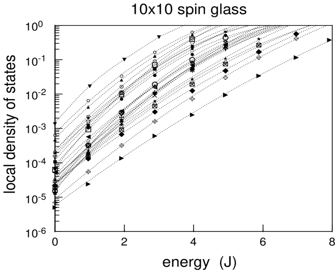
FIG. 1.: The local density of states within a pocket centered at a deep energy minimum is shown as a function of the energy in a semilogarithmic plot, for 25 different realizations of the couplings in a $10\times 10$ system. The dotted lines are fits of $\log\cal D$ to a parabola. As we have normalized the integral of the density of states to one, the differences in magnitude among the data sets directly reflect the size of the corresponding pockets.

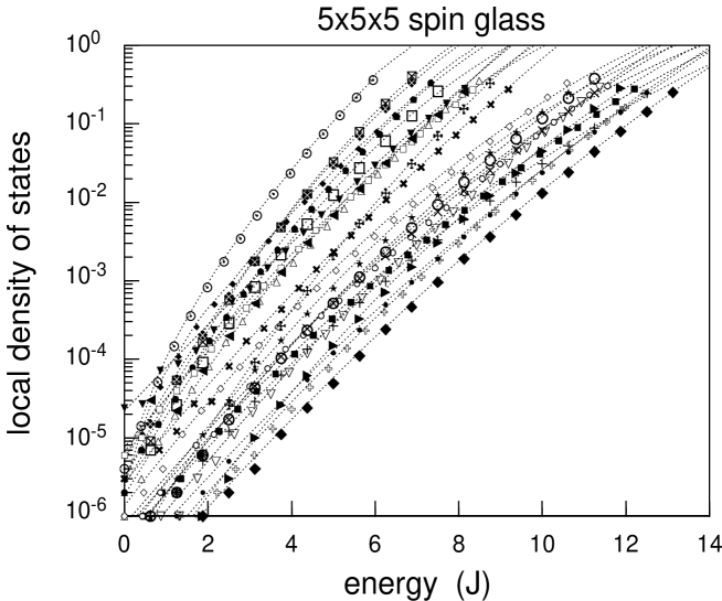
FIG. 2.: The local density of states in a pocket centered at a deep energy minimum is shown as a function of the energy in a semilogarithmic plot, for 25 different realizations of the couplings in a $5\times 5\times 5$ system. The dotted lines describe fits of $\log\cal D$ to a parabola. As the integral of the density of states is normalized to one, the differences in magnitude among the data sets reflect the size of the pockets.

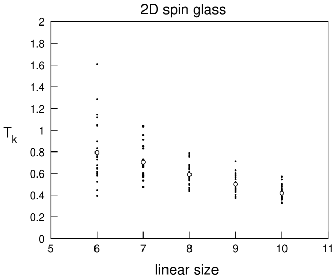
FIG. 3.: Each dot marks the estimated kinetic transition temperature $T_{k}$ of one realization of a 2D system of a given linear size. The average value of $T_{k}$ is indicated by a circle. The $T_{k}$’s are calculated by expanding $\log\cal D$ to second order in $E$ and taking the reciprocal of the coefficient of the (dominating) linear term.

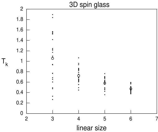
FIG. 4.: Each dot marks the estimated kinetic transition temperature $T_{k}$ of one realization of a 3D system of a given linear size. The average value of $T_{k}$ is indicated by a circle. The $T_{k}$’s are calculated by expanding $\log\cal D$ to second order in $E$ and taking the reciprocal of the coefficient of the (dominating) linear term.

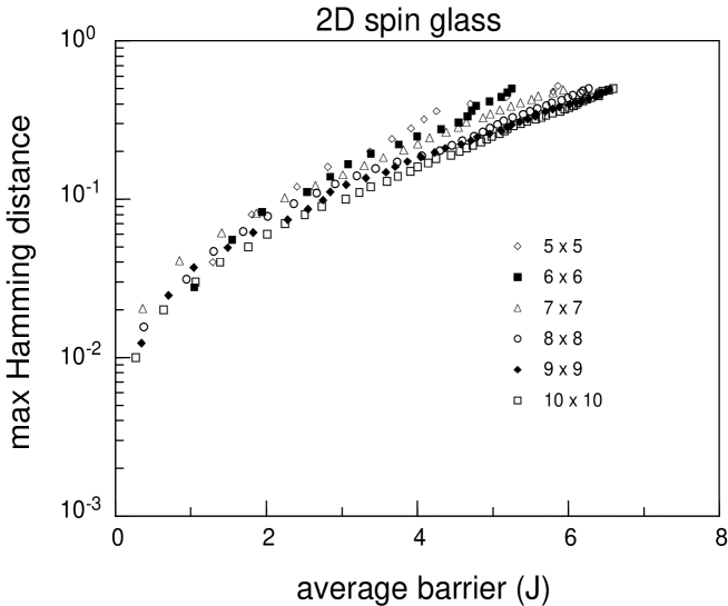
FIG. 5.: The ordinate is the largest Hamming distance to a reference state of very low energy which can be achieved without overcoming the energy barrier given by the abscissa. The data are averaged over $25$ different disorder realizations of a 2D system. Note that after a short transient, the dependence is simply exponential.

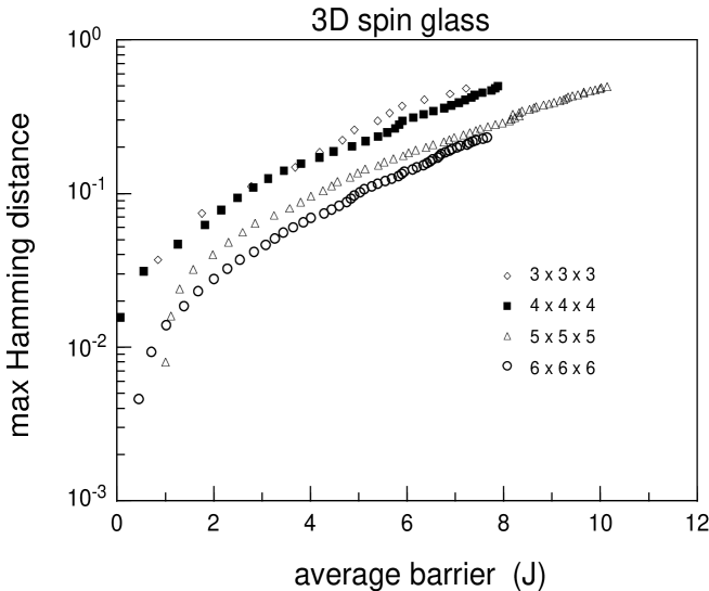
FIG. 6.: The ordinate is the largest Hamming distance to a reference state of very low energy which can be achieved without overcoming the energy barrier given by the abscissa. The data are averaged over $25$ realizations of a 3D system.

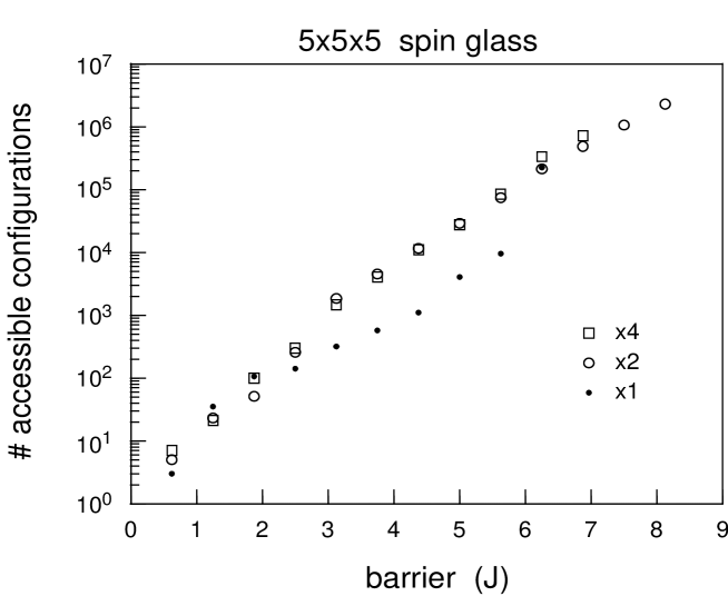
FIG. 7.: The plot shows the characteristic exponential dependence of the accessible number of states on the energy barrier for three disjoint pockets belonging to the same realization of the couplings in a $5^{3}$ system. For convenience, the data have been multiplied by different factors as indicated in the figure itself.

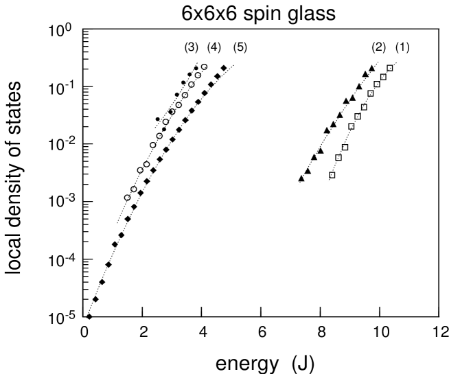
FIG. 8.: The plot describes the local density of states in a series of ‘shallow’ pockets belonging to a single $6^{3}$ system. The rightmost data set is obtained by starting the exhaustive search in a rather poor local energy minimum (energy $=-1.605716J/$spin ) and stopping it as soon as a lower energy minimum is found. This new minimum (energy $=-1.610523J/$spin ) is the starting point for the search producing the second set of data, which again stops when a better minimum is found. All shown data sets are obtained in a similar fashion. The values of the energy per spin of the reference states – besides the first two just mentioned – are $-1.632942,-1.637671$ and $-1.643615J/$spin. For convenience the energy of the very lowest energy configuration is used as the origin of the abscissa. The densities are normalized by the total number of states in the corresponding pocket.

REFERENCES

- [1] R. Palmer. Adv. Phys. 31 (1982) 669.
- [2] L. Lundgren, P. Nordblad, P. Svedlindh, and O. Beckman. J. Appl. Phys. 57 (1985) 3371.
- [3] M. Alba, M. Ocio, and J. Hammann. Europhys. Lett. 2 (1986) 45.
- [4] J. Mattsson, J.-O. Andersson and P. Svedlindh. J. Magn. Magn. Mat. 194-196 (1994) 305.
- [5] M. Lederman, R. Orbach, J. Hammann, M. Ocio, and E. Vincent. Phys. Rev. B 44 (1991) 7403.
- [6] P. Sibani and K. H. Hoffmann. Physica A 234 (1997) 751.
- [7] P. Sibani, C. Schön, P. Salamon and J.-O. Andersson. Europhys. Lett. 22 (1993) 479.
- [8] P. Sibani and P. Schriver. Phys. Rev B 49 (1994) 6667.
- [9] A. J. Bray and M. A. Moore. Phys. Rev. Lett. 58 (1987) 57.
- [10] D. S. Fisher and D. A. Huse. Phys. Rev. B 38 (1988) 373.
- [11] G. J. M. Koper and H. J. Hilhorst. J. Phys. (Paris) 49 (1988) 429.
- [12] E. Vincent, J. Hamman and M. Ocio. in : Recent Progress in Random Magnets, D. H. Ryan ed., Mc Gill University, Montreal, 1992.
- [13] M. Mezard, G. Parisi and M. A. Virasoro. Spin glass theory and beyond, World Scientific, Singapore, 1987.
- [14] C. M. Newman and D. L. Stein. Phys. Rev. Lett. 76 (1996) 515.
- [15] R.G. Palmer, D. L. Stein, E. Abrahams, P.W. Anderson. Phys. Rev. Lett. 53 (1984) 958.
- [16] Chandan Dasgupta, Shang-keng Ma and Chin-Kun Hu. Phys. Rev. B 20 (1979) 3837.
- [17] P. Sibani and J.-O. Andersson. Physica A 206 (1984) 1.
- [18] J.-O. Andersson and P. Sibani. Physica A 229 (1996) 259.
- [19] A. T. Ogielski and D. L. Stein. Phys. Rev. Lett. 55 (1985) 1634.
- [20] M. Schreckenberg. Z. Phys. B 60 (1985) 483.
- [21] S. Grossmann, F. Wegner and K. H. Hoffmann. J. Phys. Lett. (France) 46 (1985) 575.
- [22] K. H. Hoffmann, S. Grossmann, and F. Wegner. Z. Phys. B 60 (1985) 401.
- [23] P. Sibani. Phys. Rev. B 34 (1986) 3555.
- [24] P. Sibani and K. H. Hoffmann. Europhys. Lett. 16 (1991) 423.
- [25] C. Uhlig, K. H. Hoffmann and P. Sibani. Zeit. Phys. B 96 (1995) 409.
- [26] P. Sibani. Phys. Rev. B 35 (1987) 8572.
- [27] P. Sibani and K. H. Hoffmann. Phys. Rev. Lett. 63 (1989) 2853.
- [28] K. H. Hoffmann and P. Sibani. Z. Phys. B 80 (1990) 429.
- [29] Y. G. Joh, R. Orbach and J. Hamman. Phys. Rev. Lett. 77 (1996) 4648.
- [30] C. Schultze, K. H. Hoffmann, and P. Sibani. Europhys. Lett. 15 (1991) 361.
- [31] K. H. Hoffmann, S. Schubert and P. Sibani. Europhys. Lett. 38 (1997) 613.
- [32] To appreciate the significance of the entropic barriers, consider a simple ferromagnetic Ising model, which only has two equivalent energy minima. The energy barrier between them is associated to a domain wall, and scales as the linear size of the system. As the mean energy is extensive, it is an entropic barrier, i.e. the very small likelihood of focusing this energy in the right place, which accounts for the lack of ergodicity in the limit of large system size.
- [33] P. Sibani, R. Van der Pas and J. C. Schön. In preparation.
- [34] D. Vertechi and M. A. Virasoro. J. Phys. F 50 (1989) 2325.
- [35] S. F. Edwards and P. W. Anderson. J. Phys. F 5 (1975) 89.
- [36] In general, we expect that the reversal barrier should be quite close to . This can be seen as follows: by symmetry the lowest barrier needed to flip half of the spins will be the same, irrespective of whether one starts from one deep minimum or its mirror image. These two flipping procedures yield excited configurations which are each others mirror images. If they could be connected to each other with no further energy expenditure, then would follow. Unfortunately, checking this property numerically seems out of the question for all but the smallest systems. However, since both excited configurations have an energy which is rather high compared to that of single spin flips, it seems reasonable that a path between the two states can be constructed by matching pairs of consecutive flips with energy contributions of opposite sign and nearly equal magnitude.
- [37] K. Binder and A. P. Young, Rev. Mod. Phys. 58 (1986) 801.
- [38] J. Mattsson, P. Granberg, P. Nordblad, L. Lundgren, R. Loloee, R. Stubi, J. Bass and J. A. Cowen. J. Magn. Magn. Mat., 104-107 (1992) 1623.
- [39] I. A. Campbell. Phys. Rev. B 33 (1986) 3587.
- [40] W. L. McMillan. Phys. Rev. B 30 (1984) 476; Phys. Rev. B 29 (1984) 4026.
- [41] A. J. Bray and M. A. Moore. Phys. Rev. B 31 (1985) 631.
- [42] G. Parisi. Phys. Rev. Lett. 50 (1983) 46.
- [43] E. Vincent, J. P. Bouchaud, J. Hammann and F. Lefloch. Philos. Mag. B 71 (1995) 489.
- [44] J. P. Bouchaud. J. Phys. I France 2 (1994) 139.
- [45] F. Lefloch, J. Hammann, M. Ocio and E. Vincent. Europhys. Lett. 18 (1992) 647.
- [46] J.-O. Andersson, J. Mattsson and P. Svedlindh. Phys. Rev. B 48 (1994) 1063.
- [47] J. D. Reger, R. N. Bhatt and A. P. Young. Phys. Rev. Lett. 64 (1990) 1859.
- [48] In the simplest tree models the barrier confining a subtree is purely energetic. However, entropic barriers between any two given states, which shape the diffusion profile and the relaxation exponents, are also present. This is due to the fact that upon overcoming the energy barrier between the two states, an exponentially large number of other low energy states also becomes available. We also note that the kinetic transition in the models is itself a manifestation of an entropic effect: the overwhelming majority of high energy states wins over the energetic part of the Boltzmann factor.
- [49] As a check, the lid method was applied to the neighborhood of the ground state of an Ising ferromagnetic model with simple square or cubic lattice. We analyzed a , an and a system and counted , and configurations respectively. In all these cases the local density of states is almost indistinguishable from a simple exponential through the range of (low) energies considered. The ’s roughly estimated as the energy scale in this exponential are , and respectively. This must be compared with the true critical temperatures, which are in two dimensions[50] and [51] in three dimensions.
- [50] Shang-Keng Ma. Statistical Mechanics , World Scientific, 1985
- [51] C. Domb, in Phase Transitions and Critical Phenomena, Vol. 3, C. Domb and M. S. Green Eds. Academic Press, New York, 1974
- [52] J. Christian Schön. Habilitationschrift, Univ. of Bonn, and J. Christian Schön and Paolo Sibani, in preparation.