The periodic Anderson model with correlated conduction electrons

Abstract

We investigate a periodic Anderson model with interacting conduction electrons which are described by a Hubbard-type interaction of strength $U_{c}$. Within dynamical mean-field theory the total Hamiltonian is mapped onto an impurity model, which is solved by an extended non-crossing approximation. We consider the particle-hole symmetric case at half-filling. Similar to the case $U_{c}=0$, the low-energy behavior of the conduction electrons at high temperatures is essentially unaffected by the $f$ electrons and for small $U_{c}$ a quasiparticle peak corresponding to the Hubbard model evolves first. These quasiparticles screen the $f$ moments when the temperature is reduced further, and the system turns into an insulator with a tiny gap and flat bands. The formation of the quasiparticle peak is impeded by increasing either $U_{c}$ or the $c$-$f$ hybridization. Nevertheless almost dispersionless bands emerge at low temperature with an increased gap, even in the case of initially insulating host electrons. The size of the gap in the one-particle spectral density at low temperatures provides an estimate for the low-energy scale and increases as $U_{c}$ increases.

]

I Introduction

The usual explanation for the formation of heavy fermions in compounds with rare-earth or actinide elements is based on the Kondo effect.[1, 2] Thereby, the characteristic low-energy scale arises from the spin-screening of the local moments by a non-interacting electron gas. The periodic Anderson model is considered as the most promising candidate to at least qualitatively describe the rich physics of these materials. This standard scenario, however, fails to explain the heavy-fermion behavior found in the electron-doped cuprate $\rm Nd_{2-x}Ce_{x}CuO_{4}$ discovered a few years ago. [3] In particular, the estimated low-energy scale is orders of magnitude too small.[4] Since undoped $\rm Nd_{2}CuO_{4}$ is an antiferromagnetic charge-transfer insulator[5, 6] despite of one hole per unit cell, it has been suggested[4] that this discrepancy is due to the strong interactions among the electrons introduced by doping.

As regards the influence of correlated conduction electrons on the Kondo effect, up to now attention has been focused on the case of a magnetic impurity embedded in a correlated host which is either described by a Luttinger liquid in one dimension[7, 8, 9] or by some kind of Hubbard model in higher dimensions.[10, 11, 12, 13, 14, 15] In all of these cases one finds a strong dependence of the low-energy scale on the interaction strength of the conduction electrons and its increase with increasing interaction strength. For a lattice of moments hybridizing with correlated electrons only few results exist.[16, 17]

As a first step towards understanding the effect of conduction electron interactions on the formation of heavy fermions, we consider a lattice of $f$-electrons that hybridize with conduction electrons which themselves are correlated. These correlations will be described by a Hubbard-type interaction. The resulting model combines a periodic Anderson model with a Hubbard model. A limit in which one may obtain sensible results for this locally highly correlated model is the limit of large spatial dimensions.[18, 19, 20] In this limit the dynamics becomes essentially local.[19] Hence for any correlated model, a single (correlated) site may be chosen and embedded in an effective medium which has to be determined self-consistently (“dynamical mean-field theory”): The model reduces to an Anderson impurity model.[21, 22, 23] In fact, in has been shown that besides the Hubbard model[21, 24, 22, 25] the periodic Anderson model with uncorrelated conduction electrons is amenable to this limit.[26, 27, 28, 29]

In the next section we introduce the model and derive the corresponding impurity model. The impurity model is solved numerically by an extended non-crossing approximation[30, 31, 32, 33] which is derived in Sec. II as well. In Sec. III we present results for the particle-hole symmetric case at half filling. Assuming a paramagnetic ground state we study the influence of weak correlations on the one-particle spectral density and discuss how the heavy bands emerge. At low temperatures a gap forms which in the free case is related to the Kondo temperature[28] and we discuss how the size of the gap depends on the strength of the correlations of the conduction electrons. We finally conclude in Sec. IV.

II Model and Method

A The lattice Hamiltonian

In the following we consider the simplest version of the periodic Anderson model and allow for interacting conduction electrons,

$$H = H_{c}+H_{f}+H_{cf}$$ (1)

$$H_{c} = \sum_{k\sigma}(\epsilon_{k}+\epsilon_{c}-\mu)c^{\dagger}_{k,\sigma}c^{\phantom{\dagger}}_{k,\sigma}+U_{c}\sum_{i}n^{c}_{i\uparrow}n^{c}_{i\downarrow}$$ (2)

$$H_{f} = (\epsilon_{f}-\mu)\sum_{i\sigma}f^{\dagger}_{i,\sigma}f^{\phantom{\dagger}}_{i,\sigma}+U_{f}\sum_{i}n^{f}_{i\uparrow}n^{f}_{i\downarrow}$$ (3)

$$H_{cf} = V\sum_{i\sigma}\left(f^{\dagger}_{i,\sigma}c^{\phantom{\dagger}}_{i,\sigma}+c^{\dagger}_{i,\sigma}f^{\phantom{\dagger}}_{i,\sigma}\right)~{}.$$ (4)

Here, $f_{i\sigma}^{(\dagger)}$ destroys (creates) an electron in the localized $f$ orbital at site $i$ with spin $\sigma$, and $U_{f}$ is the Hubbard interaction of the localized $f$ states ($\epsilon_{f}<0$). The $c$ operators refer to the conduction electrons which are described by a Hubbard model with an interaction $U_{c}$ being typically smaller than $U_{f}$. $\mu$ denotes the chemical potential and $V$ measures the mixing between the $c$ and $f$ subsystems. In the following we will refer to the Hamiltonian (1) as “(periodic) Anderson-Hubbard model.”

In what follows we will concentrate on the one-particle spectra in a paramagnetic phase. Information on the underlying lattice will enter the dynamical mean-field equations only via the density of states of the conduction electrons.[20] For simplicity, we therefore consider a semicircular density of conduction electrons states with width $2D$ in Eq. (2)

$$\rho(z)=\frac{2}{\pi D}\sqrt{1-\left(\frac{z}{D}\right)^{2}}$$ (5)

which arises from hopping on a Bethe-lattice of coordination number $Z$ with matrix element $t=D/(2\sqrt{Z})$ in the limit $Z\to\infty$. We will use $D=1$ as unit of energy throughout this paper.

Given the non-interacting Green’s functions, $G_{0}(k,z)$,

$$G_{0}^{-1}(k,z)=\left(\begin{array}[]{c c}z-(\epsilon_{f}-\mu)&-V\\ -V&z-(\epsilon_{k}-\mu)\end{array}\right)$$ (6)

and the full Green’s function $G(k,z)$, the self-energies are defined by Dyson’s equation

$$G^{-1}(k,z) = G_{0}^{-1}(k,z)-\Sigma(k,z)$$ (7)

$$\Sigma(k,z) = \left(\begin{array}[]{c c}\Sigma_{f}(k,z)&\Sigma_{fc}(k,z)\\ \Sigma_{cf}(k,z)&\Sigma_{c}(k,z)\\ \end{array}\right)~{}.$$ (10)

B The impurity model

The dynamical mean-field theory assumes that the self-energy is a local quantity which is correct in the limit of infinite dimensions.[18, 19, 24, 20] The lattice model can then be mapped onto an impurity model[20] which is seen as follows: The self energy (10) of the lattice model (1) is given as the derivative of a functional $\Phi[G]$ of the full Green’s functions:[34]

$$\Sigma_{\mu\nu}(i,j;z)=\frac{\delta\Phi}{\delta G_{\nu\mu}(j,i;z)}~{}.$$ (11)

Here, $i$ and $j$ are real space coordinates and $\mu,\nu$ correspond to $c$ and $f$. If the self-energy of the lattice model is local, $\Phi$ depends on the local Green’s functions, $G(i,i)$, only. Thus, $\Phi$ can be generated from an impurity model. Solving the impurity model we know $\Phi$ and, hence, the self-energy as functional of the impurity Green’s function ${\cal G}$: $\Sigma[{\cal G}]=\delta\Phi/\delta{\cal G}$. We now identify ${\cal G}$ with the local Green’s function of the lattice,

$$G_{\rm loc}(z)=\frac{1}{N}\sum_{k}G(k,z)=\int d\epsilon~{}\rho(\epsilon)G(\epsilon,z)~{}.$$ (12)

Note that the $k$-dependence enters only via $\epsilon_{k}$ into $G(k,z)$, thus $G_{\rm loc}(z)$ can be expressed by an energy integration. From $G_{\rm loc}={\cal G}$, we find the actual value of $\Sigma$ from the functional equation

$$G_{\rm loc}(z) = \int d\epsilon~{}\rho(\epsilon)G(\epsilon,z)$$ (13)

$$= \int d\epsilon~{}\rho(\epsilon)\left(G_{0}^{-1}(\epsilon,z)-\Sigma[G_{\rm loc}]\right)^{-1}~{}.$$ (14)

Technically, Eq. (14) determines the free Green’s function of the impurity model which is of course not fixed by $\Phi$.

The Hamiltonian of the impurity model that generates $\Phi$ is not unique. Since $\Phi$ is the same for both impurity and lattice model, they have the same diagrammatic expansion. We therefore embed a single unit cell (a “$c$-$f$ molecule”) as impurity ($H_{\rm loc}$) in an effective medium ($H_{\rm med}$) which will be determined self-consistently:

$$H_{\rm imp} = H_{\rm loc}+H_{\rm med}$$ (15)

$$H_{\rm loc} = \tilde{\epsilon}_{c}\sum_{\sigma}c^{\dagger}_{\sigma}c^{\phantom{\dagger}}_{\sigma}+U_{c}n^{c}_{\uparrow}n^{c}_{\downarrow}+V\sum_{\sigma}\left(c^{\dagger}_{\sigma}f^{\phantom{\dagger}}_{\sigma}+{\rm H.c.}\right)$$ (17)

$$+\tilde{\epsilon}_{f}\sum_{\sigma}f^{\dagger}_{\sigma}f^{\phantom{\dagger}}_{\sigma}+U_{f}n^{f}_{\uparrow}n^{f}_{\downarrow}$$

$$H_{\rm med} = \sum_{k\sigma}E_{k}\alpha^{\dagger}_{k\sigma}\alpha^{\phantom{\dagger}}_{k\sigma}+\sum_{k\sigma}\left(W_{k}c^{\dagger}_{\sigma}\alpha^{\phantom{\dagger}}_{k\sigma}+{\rm H.c.}\right)~{}.$$ (18)

(Formally one can consider the action of the lattice model and integrate out the non-local part to arrive at an impurity action which is afterwards modelled by an Hamiltonian.[20]) Note that this choice for the impurity model differs qualitatively from the usual one for the periodic Anderson model at $U_{c}=0$.[23, 26, 27] In the case of free conduction electrons, only a single self energy exists (for the $f$-electrons) and, hence, only the $f$-orbital is coupled to an effective medium. When the conduction electrons are correlated they have a self energy, as well. Therefore, we include a $c$-orbital in the local part of $H_{\rm imp}$. We need only a single effective medium, $H_{\rm med}$, although there are two Hubbard interactions in the original Hamiltonian (1). This is due to the absence of direct $f$-$f$ hopping: The electrons explore their environment only via the $c$-orbitals. The two interactions merely show up in the internal structure of the impurity which consists of two orbitals, one of which couples to the medium. This situation is similar to the one encountered in the extended Hubbard model in Ref. [35].

We show now that the self-consistency equation (14) can be fulfilled by our impurity model (15). The impurity Green’s functions

$${\cal G}(z)=\left(\begin{array}[]{c c}{\cal G}_{f}(z)&{\cal G}_{fc}(z)\\ {\cal G}_{cf}(z)&{\cal G}_{c}(z)\end{array}\right)$$ (19)

are given by

$$\left(\begin{array}[]{c c}\omega-\tilde{\epsilon}_{f}-\Sigma_{f}(z)&-V-\Sigma_{cf}(z)\\ -V-\Sigma_{fc}(z)&\omega-\tilde{\epsilon}_{c}-\tilde{\Delta}(z)-\Sigma_{c}(z)\end{array}\right){\cal G}(z)=1~{},$$ (20)

where

$$\tilde{\Delta}(z)=\sum_{k}\frac{|W_{k}|^{2}}{z-E_{k}}~{}.$$ (21)

Equating $\cal{G}$ to the local Green’s function $G_{\rm loc}$ of the lattice model (12), which one obtains analytically due to the density of states (5), and using that both, $\tilde{\Delta}(z)$ and $G(z)\sim 1/z$ at large $|z|$, we find:

$$\tilde{\epsilon}_{f} = \epsilon_{f}-\mu$$ (22)

$$\tilde{\epsilon}_{c} = \epsilon_{c}-\mu$$ (23)

$$\tilde{\Delta}(z) = \frac{1}{4}G_{{\rm loc},c}(z)~{}.$$ (24)

The medium is determined by the $c$-Green’s function only, reflecting that there is no direct $f$-$f$ hopping.

The parameters in the impurity model (15) is thus fixed, in particular the medium $\tilde{\Delta}(z)$ is determined by the solution of the impurity model ${\cal G}_{c}(z)=G_{{\rm loc},c}(z)$.

C Solving the impurity model

We solve the impurity model (15) by extending the non-crossing approximation (NCA)[30, 31] to the case of more than two ionic propagators.[32, 33] This approach has been applied successfully to the finite-$U$ impurity Anderson model[32] where it has been shown that neglecting vertex corrections slightly underestimates the Kondo temperature, and to the Emery model within the dynamical mean-field theory.[33]

Denoting the eigenstates of the local part, $H_{\rm loc}$ by $|m\rangle$ (with $n_{m}=0\dots 4$ particles), the impurity Hamiltonian (15) is expressed in terms of Hubbard operators $X_{mn}=|m\rangle\langle n|$ as

$$H_{\rm loc} = \sum_{m=1}^{16}E_{m}X_{mm}~{}.$$ (25)

$$H_{\rm med} = \sum_{k\sigma}E_{k}\alpha^{\dagger}_{k\sigma}\alpha_{k\sigma}$$ (27)

$$+\sum_{k\sigma,mn}\left(W_{k}U^{c}_{mn\sigma}X_{mn}\alpha_{k\sigma}+{\rm H.c.}\right)$$

with $U^{c}_{mn\sigma}=\langle m|c^{\dagger}_{\sigma}|n\rangle$.

For each state $|m\rangle$ a ionic propagator is introduced

$$R_{m}(z)=\frac{1}{z-E_{m}-S_{m}(z)}$$ (28)

with spectral density $\rho_{m}(x)=-{\rm Im~{}}R_{m}(z+i0^{+})/\pi$. We assume that the corresponding self-energies $S$ are diagonal in the local basis and evaluate them in self-consistent perturbation theory to second order in the hybridization $W$ as in the usual NCA:

$$S_{m}(z) = \sum_{n,\sigma}(|U^{c}_{mn\sigma}|^{2}+|U^{c}_{nm\sigma}|^{2})\times$$ (30)

$$\quad\int_{-\infty}^{\infty}d\epsilon~{}f(\eta_{mn}\epsilon)\Delta(\epsilon)R_{n}(z+\eta_{mn}\epsilon)~{}.$$

Here $\eta_{mn}=-1(+1)$ if the particle number in $|m\rangle$ is higher (lower) than in $|n\rangle$, $f(z)=[\exp(\beta z)+1]^{-1}$ is the Fermi function, and $\Delta=-{\rm Im~{}}\tilde{\Delta}/\pi$. The $c$- and $f$-Green’s functions are given by

$$G_{c(f)}(z)=\sum_{mn}|U^{c(f)}_{mn,\uparrow}|^{2}\langle\langle X_{mn};X_{nm}\rangle\rangle_{z}$$ (31)

Within the NCA the Green’s functions $\langle\langle X_{mn};X_{nm}\rangle\rangle_{z}$ are expressed by the ionic propagators[31]

$$\langle\langle X_{mn};X_{nm}\rangle\rangle_{z}=$$ (33)

$$\frac{1}{Z}\int dx~{}e^{-\beta x}[\rho_{m}(x)R_{n}(x+z)-\rho_{n}(x)R_{m}(x-z)]$$

and

$$Z=\sum_{m}\int dx~{}e^{-\beta x}\rho_{m}(x)~{}.$$ (34)

In the symmetric, half-filled case there are only 6 independent propagators due to particle-hole and spin symmetry. The coupled integral equations (28) and (30) are solved numerically by introducing defect propagators[36] and making use of the fast Fourier transformation.[33]

III Results

In the following we consider the symmetric model ($\epsilon_{c}=-U_{c}/2$, $\epsilon_{f}=-U_{f}/2$) at half-filling ($n_{c}+n_{f}=2$). Due to particle-hole symmetry the chemical potential is 0.

We chose $U_{f}=5$ in all our calculations so that the $f$-level is well outside of the conduction band. Our investigations were restricted mostly to those values of $U_{c}$ for which the Hubbard model for the conduction electrons is metallic (for the semielliptic density of states (5) we found $U_{\rm crit}\sim 1.8$). The reason is that in deriving the self-consistency equations for the impurity model we assumed a paramagnetic state. Thus we typically chose $U_{c}=0.5\dots 2.0$ and $V=0.1\dots 0.4$. These values lead to small exchange couplings $J\sim 0.01\dots 0.2$ between two-particle singlet and triplet state of the $c$-$f$ molecule (see below). We deliberately chose these small values for $V$ in order to obtain “Kondo temperatures” which are small compared to the bare band-width, see Table I.

$V$	$T_{\rm K}^{\rm imp}$	$T_{\rm K}^{\rm lat}$
0.1	$1.3\times 10^{-44}$	$2.7\times 10^{-23}$
0.2	$2.5\times 10^{-12}$	$5.3\times 10^{-5}$
0.3	$3.1\times 10^{-6}$	$7.3\times 10^{-4}$
0.4	$4.9\times 10^{-4}$	$1.1\times 10^{-2}$

TABLE I.: The estimated Kondo temperatures for uncorrelated conduction electrons. $T_{\rm K}^{\rm imp}$ refers to the symmetric impurity Anderson model,[37] $T_{\rm K}^{\rm lat}$ includes the lattice enhancement factor of 2 in the exponent for the lattice case.[38, 28]

A Single-particle spectrum of the molecule

The following discussions focus on the one-particle spectral function. It is instructive to investigate this quantity first for the local problem given by $H_{\rm loc}$ in Eq. (15) in the symmetric case. Due to symmetry, we consider the photoemission spectrum only. Denoting the eigenstates and eigenenergies of $H_{\rm loc}$ by $|m\rangle$ and $E_{m}$, the one-particle Green’s function and spectral function are given by ($\mu=0$)

$$G_{c}(z) = \frac{1}{Z}\sum_{mn}e^{-\beta E_{m}}\times$$ (36)

$$\left(\frac{\langle m|c_{\uparrow}|n\rangle\langle n|c^{\dagger}_{\uparrow}|m\rangle}{z-(E_{n}-E_{m})}+\frac{\langle m|c^{\dagger}_{\uparrow}|n\rangle\langle n|c_{\uparrow}|m\rangle}{z+(E_{n}-E_{m})}\right)$$

$$A_{c}(z) = -\frac{1}{\pi}{\rm Im~{}}G_{c}(z+i0^{+})~{}.$$ (37)

At zero temperature only the ground state contributes to the sum over $m$. It contains two electrons forming a singlet

$$|\Psi_{\rm S}\rangle = \left[\frac{C_{1}}{\sqrt{2}}(c^{\dagger}_{\uparrow}f^{\dagger}_{\downarrow}-c^{\dagger}_{\downarrow}f^{\dagger}_{\uparrow})+\frac{C_{2}}{\sqrt{2}}(c^{\dagger}_{\uparrow}c^{\dagger}_{\downarrow}-f^{\dagger}_{\uparrow}f^{\dagger}_{\downarrow})\right]|0\rangle$$ (38)

$$E_{\rm S} = -\frac{U_{f}+U_{c}}{4}-\sqrt{\frac{(U_{f}+U_{c})^{2}}{16}+4V^{2}}~{}.$$ (39)

The photoemission spectrum is obtained by removing a particle, hence the final states are bonding and antibonding combination of the $c$- and $f$-orbital. To lowest order in $V$ the transition energies are given by

$$z_{c} = -\frac{U_{c}}{2}-2\frac{3U_{f}-5U_{c}}{(U_{c}+U_{f})(U_{f}-U_{c})}V^{2}$$ (40)

$$z_{f} = -\frac{U_{f}}{2}-2\frac{5U_{f}-3U_{c}}{(U_{c}+U_{f})(U_{f}-U_{c})}V^{2}~{}.$$ (41)

They correspond to the lower Hubbard bands of the $c$- and $f$-subsystem which are shifted by the hybridization $V$.

The first excited state is the two-electron triplet state (spin excitation)

$$|\Psi_{\rm T}\rangle=\frac{1}{\sqrt{2}}(c^{\dagger}_{\uparrow}f^{\dagger}_{\downarrow}+c^{\dagger}_{\downarrow}f^{\dagger}_{\uparrow})|0\rangle$$ (42)

with excitation energy

$$\Delta E=E_{\rm T}-E_{\rm S} = \sqrt{\frac{(U_{f}+U_{c})^{2}}{16}+4V^{2}}-\frac{U_{f}+U_{c}}{4}$$ (43)

$$\sim \frac{8V^{2}}{U_{f}+U_{c}}~{}.$$ (44)

At the temperatures that we investigate in the following ($T=0.5\cdots 0.001$) only these two states contribute as initial states, $|m\rangle$. The resulting photoemission spectrum of the molecule thus consists of two double peaks at $z_{c}$, $z_{c}+\Delta E$, and $z_{f}$, $z_{f}+\Delta E$ and the weight of the peaks shifted by $\Delta E$ goes to 0 as $T\to 0$.

B Single-particle spectrum of the Anderson-Hubbard model

We first consider the spectral density of the conduction electrons

$$A_{c}(z) = -\frac{1}{\pi}{\rm Im~{}}G_{{\rm loc},c}(z+i0^{+})$$ (45)

$$= -\frac{1}{\pi}\sum_{k}{\rm Im~{}}G_{c}(k,z+i0^{+})$$ (46)

which corresponds to photoemission and inverse photoemission spectra.

FIG. 1.: Spectral density $A_{c}(z)$ for $U_{c}=1$, $V=0.2$, $U_{f}=5$ at different temperatures

A typical result for $A_{c}(z)$ is shown in Fig. 1 for different temperatures ($U_{c}=1$, $V=0.2$). At high temperatures ($T=0.5$) we obtain two broad maxima located at $\sim\pm U_{c}/2$ which correspond to upper and lower Hubbard band of the $c$-subsystem. When lowering the temperature ($T\lesssim 0.1$), a peak at the chemical potential ($z=0$) arises. This is the well-known quasiparticle peak belonging to the Hubbard model of the host electrons, $H_{c}$. [22, 24, 25] In this temperature regime the $f$- and $c$-subsystems are almost independent. The influence of the $f$-states on the $c$-spectra is given only by the tiny structure at $z\sim\pm U_{f}/2=\pm 2.5$.

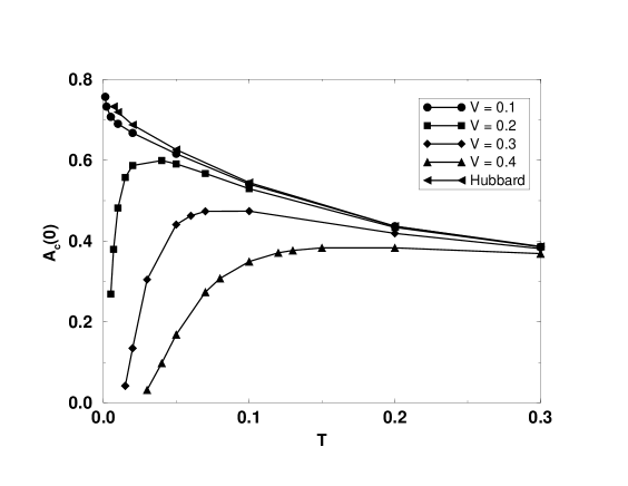
FIG. 2.: Spectral weight of the conduction electrons at the chemical potential, $A_{c}(0)$, for $U_{c}=1$ vs. temperature

The separation of the two subsystems is indicated in Fig. 2 as well where we compare the spectral weight at the chemical potential for different values of the $c$-$f$ hybridization $V$ and the pure $c$-Hubbard model ($V=0$): At high to moderate temperatures the spectral weight of the Anderson-Hubbard model follows the one of the pure Hubbard model.

In Fig. 2 we also see that this behavior does not extend to low temperatures. At a certain temperature, which depends on $V$, the spectral weight no longer follows the quasiparticle peak of the Hubbard model but drops to zero. As seen in Fig. 1 indeed a gap occurs and sharp structures emerge close to the chemical potential when the temperature falls below $T\lesssim 0.04$. This resembles the Anderson model with uncorrelated conduction electrons.[28] There, at $T<T_{0}$ where $T_{0}$ is a characteristic temperature related to the Kondo temperature, the Kondo effect leads to a resonance at the chemical potential. These dynamically generated local states cross the conduction-band states and one finds a splitting of the conduction band with a gap at the position of the resonance. Due to particle-hole symmetry, this feature occurs at the chemical potential and the system becomes an insulator.[39]

A similar behavior is found in the case of interacting conduction electrons. In order to see that indeed flat bands occur close to the chemical potential we inspect the $k$-dependent spectral function

$$A_{c}(k,z)=-\frac{1}{\pi}{\rm Im~{}}G_{c}(k,z)~{}.$$ (47)

From the self-consistency equation (14) and Eq. (7) we find

$$G_{c}(k,z)=\frac{1}{G_{{\rm loc},c}^{-1}(z)-\epsilon_{k}+\frac{1}{4}G_{{\rm loc},c}(z)}~{}.$$ (48)

Since $A_{c}(k,z)$ depends on $k$ only via $\epsilon_{k}$, we plot $A_{c}(k,z)$ for different $\epsilon_{k}=-1\dots 1$ in Fig. 3.

FIG. 3.: Spectral function $A_{c}(k,z)$ for $U_{c}=1$, $V=0.2$ and different values of $\epsilon(k)$. a. $T=0.3$, b. $T=0.05$, c. $T=0.005$

At high temperatures ($T=0.3$, Fig. 3a.) the features are very broad and we basically see the Hubbard bands for the $c$-subsystem at $\sim U_{c}/2$ as well as for the $f$-subsystem at $\sim U_{f}/2$ which weakly admix to the $c$ spectra. At intermediate temperatures ($T=0.1\dots 0.02$, $T=0.05$ is shown in Fig. 3b.) spectral weight is found at the chemical potential as well and we may trace the quasiparticle band of the Hubbard model. When the temperature is decreased below 0.015 ($T=0.005$, Fig. 3c.) these peaks split, a small gap opens and the newly emerged peaks show a weak dispersion at the chemical potential. The transition occurs rather quickly: Whereas at $T=0.015$ only the peak at $\epsilon_{k}=0$ is split and the band follows the quasiparticle band of the Hubbard band elsewhere, two separated bands already emerged at $T=0.01$. Due to their weak dispersion at the chemical potential we expect that they will lead to heavy bands upon doping. At higher energies these new bands merge in the previous quasiparticle bands of the Hubbard model.

These findings fit qualitatively to the scenario of the Anderson model with uncorrelated conduction electrons described above[28] and to the results of the slaved-boson mean-field treatment.[40] In the latter, the free conduction bands hybridize with a strongly renormalized (reduced) coupling to an effective $f$-level at the chemical potential. This leads to weakly dispersive bands at low energies merging in the original bands at high energies. In the Anderson-Hubbard model the new bands merge in the former quasiparticle band of the $c$-Hubbard model at high energies. We conclude that these quasiparticles take the role of the free conduction electrons in the dynamical screening of the $f$-moments leading to the resonance at the chemical potential. This interpretation does not contradict previous results on a single impurity embedded in a correlated host.[14] There it turned out that a variational ansatz in the spirit of Varma and Yafet[41] which uses quasiparticles for the screening of the $f$-moment instead of bare electrons is not sufficient to find the correct Kondo temperature. This holds due to importance of the renormalization of the $c$-$f$ exchange interaction and does not imply that the quasiparticle picture is not valid in describing the screening process.

When the interaction strength of the conduction electrons is increased to $U_{c}=1.5$, no qualitative changes occur at first sight.

FIG. 4.: Spectral density $A_{c}(z)$ for $U_{c}=1.5$, $V=0.2$, $U_{f}=5$ at different temperatures

In Fig. 4 we show the $c$-spectra at various temperatures for $U_{c}=1.5$ and $V=0.2$. Again, the $c$- and $f$-subsystem are separated at high temperatures and a quasiparticle peak of the $c$-Hubbard model evolves first. At low temperatures a Kondo resonance is formed at the chemical potential with hybridizes with the quasiparticle band, a gap opens and we find bands with a weak dispersion. When compared to $U_{c}=1$, we find that the gap has increased. This indicates that the hybridization of the quasiparticle band with the dynamically generated states has increased.

FIG. 5.: Spectral density $A_{c}(z)$ for $U_{c}=1.5$, $V=0.3$, $U_{f}=5$ at different temperatures

However, as demonstrated in Fig. 5, a quasiparticle peak does not always occur in the intermediate temperature range even though the bare conduction electrons are metallic: Increasing the $c$-$f$ mixing to $V=0.3$, the system becomes directly insulating although $U_{c}=1.5<U_{\rm crit}$.

FIG. 6.: Spectral weight of the conduction electrons at the chemical potential, $A_{c}(0)$, for $U_{c}=1.5$ vs. temperature

Figure 6 illustrates that it depends on the value of $V$ whether the quasiparticle peak shows up or not. We conclude that part of the strong correlation on the $f$-orbital is effectively inherited by the $c$-orbital via the hybridization $V$. A similar effect has been observed and discussed for a different model in Ref. [42].

Although no quasiparticle peak corresponding to the conduction electrons emerges in Fig. 5, we still recover the Anderson scenario described above when decreasing the temperature, i.e., a gap opens and peaks arise close to it at low temperatures $T\sim 0.04$. It appears that we do not need pre-formed quasiparticles in order to screen the $f$-moments which in turn leads to the Kondo resonance. Note however, that there is finite spectral weight at the chemical potential.

FIG. 7.: Comparison of the spectral function $A_{c}(k,z)$ of the Anderson-Hubbard model ($U_{c}=1.5$, $V=0.2$, solid lines) to the Hubbard model ($U_{c}=1.5$, dashed lines, multiplied by $-1$) at a. $T=0.07$ and b. $T=0.04$.

This is better seen in the $k$-resolved spectral function $A_{c}(k,z)$ in Fig. 7 where we display $A_{c}(k,z)$ for two different temperatures for the Anderson-Hubbard ($U_{c}=1.5,V=0.3$) and the Hubbard model ($U=1.5$). For the Hubbard model we find a peak crossing the chemical potential at $T=0.07$ (Fig. 7a.). It corresponds to the quasiparticle peak of the Hubbard model being formed at this temperature. The Anderson-Hubbard model, however, exhibits no structure crossing the chemical potential. Note that upper and lower Hubbard bands of the Anderson-Hubbard model are in agreement with those of the pure Hubbard model. At $T=0.04$ (Fig. 7b.) the Anderson-Hubbard model shows two flat bands at the chemical potential. The peaks are most pronounced close to chemical potential. In contrast to the case of small $U_{c}$ ($U_{c}=1$ discussed above) the corresponding bands do not merge the quasiparticle band of the Hubbard model. This indicates a large effective hybridization between quasiparticle and dynamically generated states at the chemical potential. To a lesser degree this behavior is also observed for $U_{c}=1.5$ and $V=0.2$ ($A_{c}(k,z)$ not shown). We conclude that the effective hybridization increases as both $U_{c}$ and $V$ increase. Considering again Fig. 7a., we find that the difference between Hubbard and Anderson-Hubbard model at high temperatures is related to the onset of the heavy bands which are thus already seen at comparatively high temperatures.

We finally turn to the case where the bare $c$-subsystem is insulating, i.e., $U_{c}>U_{\rm crit}$.

FIG. 8.: Spectral density $A_{c}(z)$ for $U_{c}=2$, $V=0.3$, $U_{f}=5$

For $U_{c}=2$ a shoulder in the spectral function emerges at the edge Hubbard band towards the chemical potential when the temperature is lowered (Fig. 8).

FIG. 9.: Comparison of the $c$ spectral function $A_{c}(k,z)$ of the Anderson-Hubbard model ($U_{c}=2$, $V=0.3$, $U_{f}=5$, solid lines) to the Hubbard model ($U_{c}=2$, dashed lines, multiplied by $-1$) at $T=0.065$

That this feature is indeed caused by the $f$-subsystem is demonstrated in Fig. 9 where we compare $A_{c}(k,z)$ for the Anderson-Hubbard model and the pure Hubbard model. Whereas the structures corresponding to the Hubbard bands roughly agree, the Anderson-Hubbard model shows an additional peak at the low-energy edge of the Hubbard bands. This is unexpected because the $c$-subsystem is insulating and provides no quasiparticles which could screen the $f$-moment and the resulting spectra should resemble the one of the $c$-$f$ molecule described in Sec. III A. We do not believe that this shoulder is spurious since increasing the energy resolution which allows to proceed to lower temperatures did not change the shoulder. However, we can not exclude a principle failure of the extended NCA as it is well-known that the NCA fails to converge when the system becomes insulating.[43] On the other hand, the spectral weight at the chemical potential is not exactly zero. Similar to the case $U_{c}=1.5$, $V=0.3$ discussed above, this small, but finite spectral weight could be sufficient to dynamically generate states at the chemical potential which result in a heavy band via hybridization as previously. To clarify this situation, it is mandatory to employ other numerical methods for solving the impurity model. If the picture presented above is valid, the effective hybridization must be large compared to the metallic cases so that the new bands are pushed towards the Hubbard bands. Note that the new peaks approach, but not merge in the Hubbard bands whereas they merged in the quasiparticle bands in the metallic cases ($U_{c}=1$, and $U_{c}=1.5$, $V\lesssim 0.2$).

C Hybridization gap

In this section we focus on the gap which opens at low temperatures. We determine the size of the gap, $\Delta$, as twice the distance between zero frequency and the first maximum close to the chemical potential.[28]

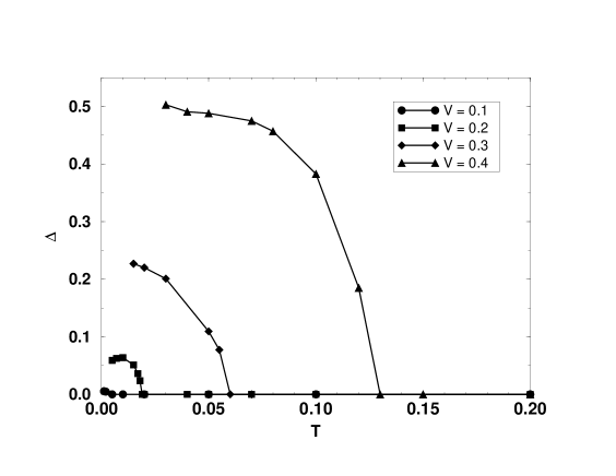
FIG. 10.: Gap in the spectral density vs. temperature. The gaps are obtained from the two maxima in $A_{c}(z)$ for $U_{c}=1$ and different hybridizations $V$

In Fig. 10, where we plot the gap $\Delta$ vs. temperature for different hybridizations $V$, we observe that the gap opens quickly when the temperature is reduced and we define $T_{0}$ as the temperature where the gap opens. One expects that $T_{0}$ is related to the energy difference, $\Delta E$, of singlet and triplet states in the local problem, see Sec. III A. Indeed, we observe in Figs. 4 and 5 that the gap opens roughly in the same temperature regime where the $f$-peak at $z\sim\pm U_{f}/2$ splits, i.e., where the states $|\Psi_{\rm S}\rangle$ and $|\Psi_{\rm T}\rangle$ become distinguishable in the photoemission of the lattice. We extract this splitting of the $f$-peak, $\Delta E_{\rm lat}$ from the spectral function of the lattice model (if visible) and compare it to the corresponding splitting, $\Delta E_{\rm loc}$ for the $c-f$ molecule [cf. Eq. (44)] in Fig. 11 for different values of $U_{c}$ and $V=0.3$.

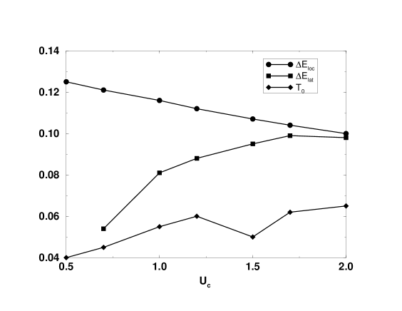
FIG. 11.: Splitting of the $f$ peak in the molecule and lattice, and $T_{0}$ vs. $U_{c}$ at $V=0.3$

Surprisingly we find that while both splittings are of the same order of magnitude, they depend differently on $U_{c}$: When $U_{c}$ increases, $\Delta E_{\rm lat}$ increases, whereas $\Delta E_{\rm loc}$ decreases.

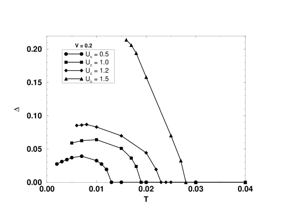
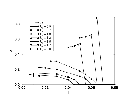
FIG. 12.: Gap in the spectral density vs. temperature. The gaps are obtained from the two maxima in $A_{c}(z)$ for different interaction strength $U_{c}$ and a. $V=0.2$ and b. $V=0.3$

In Fig. 12 we plot the gap vs. temperature for different values of $U_{c}$ and $V=0.2,~{}0.3$. In general, the temperature $T_{0}$ at which the gap sets in increases with $U_{c}$, but deviations occur: When $V=0.3$, $U_{c}=1.5$ and $1.7$ do not fit into this scheme. However, one should bear in mind that the onset of the gap formation as we measure it, depends also on the shape of the spectrum. As is seen from Fig. 11, $T_{0}$ is of the same order of magnitude as $\Delta E_{\rm lat}$ and its general behavior agrees with $\Delta E_{\rm lat}$ and is thus opposed to $\Delta E_{\rm loc}$.

We now turn to the size of the gap. It has been shown for the Anderson model with free conduction electrons that this quantity determines the low-temperature thermodynamics in the limit of infinite dimensions.[44, 45, 28] The gaps in the local spin and charge excitation spectra were found to be of the same order of magnitude as the gap in the density of states. The latter thus provides a measure of the low-temperature scale (“Kondo temperature”). From Fig. 12 we extract that the size of the gap has not yet converged at the lowest temperatures where our extended NCA ceases to converge. Nevertheless, we can draw some qualitative conclusions: The size of the gap increases systematically as $U_{c}$ increases.

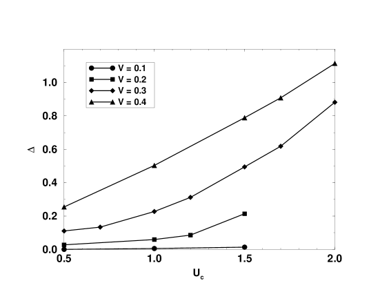
FIG. 13.: Gap in the spectral density vs. $U_{c}$. The gaps correspond to the lowest temperatures reached.

This is also deduced from Fig. 13 where we plotted the gap at the lowest temperature we could reach for each pair $(U_{c},V)$ vs. the strength $U_{c}$ of the Hubbard interaction of the conduction electrons. This procedure implies that the points shown correspond to different temperatures. Note that the magnitude of $\Delta$ varies much stronger with $U_{c}$ and $V$ compared to $T_{0}$ or $\Delta E$.

IV Conclusions

In conclusion, we studied the influence of interactions among the conduction electrons on the low-temperature behavior of the periodic Anderson model. In the dynamical mean-field theory the model is mapped onto a generalized Anderson impurity model that couples the orbitals of a single unit cell to an effective medium which has to be determined self consistently. The impurity model was solved numerically by an extended non-crossing approximation.

For weakly interacting conduction electrons we found that at high temperatures the $c$- and $f$-subsystems are almost separated as in the case of free conduction electrons. Decreasing temperature then first leads to the formation of quasiparticles in the $c$-subsystem as in the bare Hubbard model. When the temperature is reduced further, the quasiparticle band splits, a tiny gap opens and the system turns into an insulator. As in the case of free conduction electrons, the gap is formed by the level crossing of the quasiparticle (Hubbard) band and the resonance which arises at the chemical potential from the Kondo-like screening of the $f$-moments. We observed that the quasiparticles play an essential role in this screening. The resulting two bands have a weak dispersion close to the gap and we expect that they turn into heavy bands upon doping.

When the correlations of the conduction electrons become stronger, the low-temperature gap increases. This can be interpreted as increasing the effective hybridization between the quasiparticle states at the chemical potential and the dynamically generated states which leads to a larger gap and is qualitatively in agreement with results found for impurity models. For the latter case, the main effect of the (small) interaction was to renormalize and increase the exchange interaction.[14]

It turned out, however, that pre-formed quasiparticles within the $c$-subsystem are not prerequisite for the emergence of heavy bands. When increasing the $c$-$f$ hybridization, the $c$ orbitals seem to inherit correlations from the $f$ orbitals and a quasiparticle peak is no longer formed in the spectral density at intermediate temperatures, although the spectral weight at the chemical potential does not vanish. Nevertheless, we observed heavy bands at low temperatures in the one-particle spectra.

Even when the (bare) $c$-system is insulating, it is influenced by the $f$-system at low temperatures: A shoulder forms at the edge of the Hubbard band which shows weak dispersion. This is surprising since the bare $c$-system provides no quasiparticles which could screen the $f$-moments and the $c$ spectral weight close to the chemical potential is small. However, we can not exclude that this result is an artefact of our method to solve the impurity problem and further investigations are necessary to decide upon this question.

Finally, we investigated the hybridization gap which occurs at low temperatures. When increasing the Coulomb interaction among the conduction electrons the temperature at which the gap opens increases. This temperature is related to the splitting of the $f$-peak in the spectrum which results from singlet and triplet states in the $c$-$f$ molecule. However, we found that this splitting depends oppositely on the interaction strength in the lattice and in the molecule. The low-temperature thermodynamics in infinite dimensions scales with the size of the gap.[28] This quantity therefore provides a measure for the “Kondo temperature.” In agreement with impurity models, this gap increases as the correlations among the conduction electrons become stronger.

- [1] P. Fulde, J. Keller, and G. Zwicknagl, in Solid state physics, edited by H. Ehrenreich and D. Turnbell (Academic Press, San Diego, 1988), Vol. 41, pp. 1–150.
- [2] A. C. Hewson, The Kondo Problem to Heavy Fermions (Cambridge University Press, Cambridge, 1993).
- [3] T. Brugger et al., Phys. Rev. Lett. 71, 2481 (1993).
- [4] P. Fulde, V. Zevin, and G. Zwicknagl, Z. Phys. B 92, 133 (1993).
- [5] S. Skanthakumar et al., Physica C 160, 124 (1989).
- [6] S. B. Oseroff et al., Phys. Rev. B 41, 1934 (1990).
- [7] A. Furusaki and N. Nagaosa, Phys. Rev. Lett. 72, 892 (1994).
- [8] Y. M. Li, Phys. Rev. B 52, R6979 (1995).
- [9] P. Fröjdh and H. Johannesson, Phys. Rev. B 53, 3211 (1996).
- [10] T. Schork and P. Fulde, Phys. Rev. B 50, 1345 (1994).
- [11] G. Khaliullin and P. Fulde, Phys. Rev. B 52, 9514 (1995).
- [12] J. Igarashi, T. Tonegawa, M. Kaburagi, and P. Fulde, Phys. Rev. B 51, 5814 (1995).
- [13] J. Igarashi, K. Murayama, and P. Fulde, Phys. Rev. B 52, 15966 (1995).
- [14] T. Schork, Phys. Rev. B 53, 5626 (1996).
- [15] X. Wang, preprint (unpublished).
- [16] N. Shibata, T. Nishino, K. Ueda, and C. Ishii, Phys. Rev. B 53, R8828 (1996).
- [17] K. Itai and P. Fazekas, Phys. Rev. B 54, R752 (1996).
- [18] W. Metzner and D. Vollhardt, Phys. Rev. Lett. 62, 324 (1989).
- [19] E. Müller-Hartmann, Z. Phys. B 74, 507 (1989).
- [20] A. Georges, G. Kotliar, W. Krauth, and M. Rozenberg, Rev. Mod. Phys. 68, 13 (1996).
- [21] F. J. Ohkawa, J. Phys. Soc. Jpn. 60, 3218 (1991).
- [22] M. Jarrell, Phys. Rev. Lett. 69, 168 (1992).
- [23] A. Georges, G. Kotliar, and Q. Si, Int. J. Mod. Phys. 6, 705 (1992).
- [24] F. J. Ohkawa, J. Phys. Soc. Jpn. 61, 1615 (1992).
- [25] A. Georges and G. Kotliar, Phys. Rev. B 45, 6479 (1992).
- [26] F. J. Ohkawa, Phys. Rev. B 46, 9016 (1992).
- [27] M. Jarrell, H. Akhlaghpour, and T. Pruschke, Phys. Rev. Lett. 70, 1670 (1993).
- [28] M. Jarrell, Phys. Rev. B 51, 7429 (1995).
- [29] T. Saso and M. Itoh, Phys. Rev. B 53, 6877 (1996).
- [30] H. Keiter and J. C. Kimball, Phys. Rev. Lett. 25, 672 (1970).
- [31] N. E. Bickers, Rev. Mod. Phys. 59, 845 (1987).
- [32] T. Pruschke and N. Grewe, Z. Phys. B 74, 439 (1989).
- [33] P. Lombardo, M. Avignon, J. Schmalian, and K.-H. Bennemann, Phys. Rev. B 54, 5317 (1996).
- [34] A. A. Abrikosov, L. P. Gorkov, and I. E. Dzialoshinski, Methods of Quantum Field Theory in Statistical Physics (Pergamon, Elmsford, NY, 1965).
- [35] Q. Si and G. Kotliar, Phys. Rev. B 48, 13881 (1993).
- [36] N. E. Bickers, D. L. Cox, and J. W. Wilkins, Phys. Rev. B 36, 2036 (1987).
- [37] A. M. Tsvelick and P. B. Wiegmann, Adv. Phys. 32, 453 (1983).
- [38] T. M. Rice and K. Ueda, Phys. Rev. B 34, 6420 (1986).
- [39] K. Yamada and K. Yoshida, in Theory of Heavy Fermions and Valence Fluctuations, Vol. 62 of Springer Series in Solid-State Sciences, edited by T. Kasuya and T. Saso (Springer, Berlin, 1985), pp. 183–194.
- [40] D. M. Newns and N. Read, Adv. Phys. 36, 799 (1987).
- [41] C. M. Varma and Y. Yafet, Phys. Rev. B 13, 2950 (1976).
- [42] S. Blawid, H. A. Tuan, T. Yanagisawa, and P. Fulde, Phys. Rev. B 54, 7771 (1996).
- [43] T. Pruschke, D. L. Cox, and M. Jarrell, Phys. Rev. B 47, 3553 (1993).
- [44] T. Mutou and D. S. Hirashima, J. Phys. Soc. Jpn. 63, 4475 (1994).
- [45] T. Mutou and D. S. Hirashima, J. Phys. Soc. Jpn. 64, 4799 (1995).