1 Introduction

Non-hermitean random matrix theory [1] has been applied recently to a number of interesting physical situations. An interesting issue among these physical situations is the study of localization-delocalization transitions in non-hermitean random Hamiltonians. The earliest discussion of localization in the context of a non-hermitean hydrodynamics problem appears to be in [2]. Later on, Hatano and Nelson [3] have mapped the problem of the vortex line pinning in superconductors to a problem involving a non-hermitean random Hamiltonian. When a current is passed through a superconductor, vortex lines tend to drift in a direction perpendicular to the current, but this tendency is counteracted by impurities on which the vortex lines are pinned. It is expected that at some critical current the vortex lines become unpinned or delocalized. In the simplest model of this problem, the physics is modelled by a quantum particle hopping on a ring, whose rightward (or counterclockwise) hopping amplitude $te^{h}/2$ is different from its leftward hopping amplitude $te^{-h}/2$. Note that $ih$ may be thought of as an imaginary gauge field. On each site of the ring is a random potential $w_{i}$ which tries to trap the particle. The Hamiltonian

$$H=H_{0}+W$$ (1)

is thus the sum of the deterministic non-hermitean hopping term

$$H_{0ij}={t\over 2}\left(e^{h}~{}\delta_{i+1,j}+e^{-h}~{}\delta_{i,j+1}\right)\quad,\quad i,j=1,\cdots N$$ (2)

(with the obvious periodic identification $i+N\equiv i$ of site indices) and the hermitean random potential term

$$W_{ij}=w_{i}~{}\delta_{i,j}\,.$$ (3)

The number of sites $N$ is understood to be tending to infinity. This problem has been studied by a number of authors [4, 5, 6, 7] following Hatano and Nelson. Note that the Hamiltonian not only breaks parity as expected but is non-hermitean, and thus has complex eigenvalues. It is represented by a real non-symmetric matrix, with the reality implying that if $E$ is an eigenvalue, then $E^{*}$ is also an eigenvalue.

With no impurities ($w_{i}=0$) the Hamiltonian is immediately solvable by Bloch’s theorem with the eigenvalues

$$E_{n}=t~{}{\rm cos}~{}({2\pi n\over N}-ih)\,,\quad(n=0,1,\cdots,N-1)\,,$$ (4)

tracing out an ellipse. The corresponding wave functions $\psi^{(n)}_{j}\sim{\rm exp}~{}2\pi inj/N$ are obviously extended. Note that in the limit of zero non-hermiticity ($h=0$) the ellipse collapses to a segment on the real axis as expected. With impurities present the spectrum can be obtained by numerical work as was done extensively by Hatano and Nelson and as is shown in Fig. 1.

Figure 1: The spectrum of the Hamiltonian in Eq. (1) for $h=0.5$, $t=2$ and $N=400$ sites. Shown here is the spectrum for one particular realization of site energies taken from a flat distribution with $-2\leq w_{i}\leq 2$. A finite fraction of eigenvalues has clearly snapped onto the real axis. (The coordinate axes have been suppressed to make the appearance of the snapped eigenvalues clearer.)

Two “wings” have emerged out of the two ends of the ellipse. Some eigenvalues have become real. Evidently, the “forks” where the two wings emerge out of the ellipse represent a non-perturbative effect, and cannot be obtained by treating the impurities perturbatively. It is thus something of a challenge to obtain the two wings analytically. In this paper, we address this and other problems.

As discussed in Section 6 of [5] this behavior could be understood qualitatively by a simple example. In ordinary hermitean quantum mechanics, it is a familiar textbook dictum that nearby eigenvalues repel. In contrast, two nearby eigenvalues in the complex plane, separated along the imaginary direction, attract each other under a hermitean perturbation. To see this consider the $2\times 2$ matrix

$$\left(\begin{array}[]{cc}i\epsilon&0\\ {}\hfil&{}\hfil\\ 0&-i\epsilon\end{array}\right)+\left(\begin{array}[]{cc}0&w\\ {}\hfil&{}\hfil\\ w&0\end{array}\right)$$

with eigenvalues are $\pm i\sqrt{\epsilon^{2}-w^{2}}$. Thus, for $w<\epsilon$, the original eigenvalues $\pm i\epsilon$ attract each other, but remain on the imaginary axis. However, as soon as $w\geq\epsilon$, they snap onto the real axis and start repelling each other. Let us start with the ellipse in the absence of impurities. Near each tip of the ellipse, there is a pair of eigenvalues separated slightly along the imaginary direction and lying on opposite sides of the real axis. They attract each other and thus approach the real axis, but as soon as the two “friends” arrive on the real axis, they immediately repel each other (as well as the eigenvalue already on the real axis.) Obviously, this process repeats itself with the next pair of eigenvalues, and thus leads to the formation of the wings.

Hatano and Nelson emphasized that $H_{0}$ has a special property, namely that by a (non-unitary) gauge transformation, all the non-hermiticity can be concentrated on one arbitrarily chosen bond, without changing the spectrum. This leads to an extraordinarily simple argument that the states corresponding to complex eigenvalues are extended, that is, delocalized. Let $H\psi=E\psi$. Assume that $\psi$ is localized around some site $j$. We can always gauge the non-hermiticity to a link which is located arbitrarily far away from the site $j$, where $|\psi|$ is exponentially small. Thus, if we cut the ring open at that link, the effect on the Schrödinger equation would be exponentially small, and would vanish completely in the limit $N\rightarrow\infty$. It follows from this simple argument that if we replace the periodic boundary condition in solving $H\psi=E\psi$ by an open chain boundary condition, the localized part of the spectrum of (1) would not be affected. But for $H$ with an open chain boundary condition, the gauge transformation just mentioned may be used to gauge away the non-hermiticity completely, meaning that the Hamiltonian is in effect hermitean with real eigenvalues. We thus conclude that all localized eigenstates of (1) correspond to real eigenvalues (in the large $N$ limit.) In other words, the states corresponding to complex eigenvalues are extended, that is, delocalized.

Remarkably, non-hermitean localization theory is simpler in this respect than the standard hermitean localization theory of Anderson and others [8]. To understand the localization transition, one has to study only the density of eigenvalues, or equivalently, the one-point Green’s function, rather than the two-point Green’s function.

2 The single impurity case

In this section our philosophy is to find the simplest version of the hopping model described in the Introduction which we can solve exactly, but yet manages to capture the essential physics involved, including the non-perturbative emergence of the two “wings” along the real axis. The desired simplification is to replace the $N$ random impurities in (3) by a single impurity. With this simplification we do not need to specify the precise form of the non-hermitean $H_{0}$ beyond assuming that it is translationally invariant. We thus replace the $W_{i,j}$ in (3) by

$$W_{i,j}=w\,\delta_{i,1}\,\delta_{j,1}$$ (6)

where $w$ is drawn from some probability distribution $P(w)$.

Our task is to calculate the averaged Green’s function

$$G(z,z^{*})=\langle{1\over N}~{}{\rm tr}~{}{1\over z-H_{0}-W}\rangle$$ (7)

of the random Hamiltonian $H=H_{0}+W$, from which we may calculate the eigenvalue density of $H$.

Away from the location of the spectrum of $H_{0}$ in the complex $z$ plane we expand (7) in powers of $1/(z-H_{0})$, and thus obtain

$$G(z)=G_{0}(z)-{1\over N}\left[{\partial\over\partial z}\left({1\over z-H_{0}}\right)_{1,1}\right]\sum_{k=1}^{\infty}\langle w^{k}\rangle\left[\left({1\over z-H_{0}}\right)_{1,1}\right]^{k-1}$$ (8)

where

$$G_{0}(z)=\langle{1\over N}~{}{\rm tr}~{}{1\over z-H_{0}}\rangle$$ (9)

is the Green’s function of $H_{0}$. Due to the translational invariance of $H_{0}$ we have

$$\left({1\over z-H_{0}}\right)_{1,1}=G_{0}(z)$$

and so

$$G(z) = G_{0}(z)-{1\over N}~{}{\partial G_{0}(z)\over\partial z}\sum_{k=1}^{\infty}\langle w^{k}\rangle\left[G_{0}(z)\right]^{k-1}$$ (10)

$$= G_{0}(z)-{1\over N}~{}{\partial G_{0}(z)\over\partial z}~{}\langle{w\over 1-wG_{0}(z)}\rangle\,.$$

Observe that the effect of the single impurity on the Green’s function is of order $1/N$, as should be expected.

We stress again that up to this point we did not adhere to any specific translationally invariant $H_{0}$ nor did we specify any particular probability distribution $P(w)$ in our derivation of (10). We also note that our derivation is exact for any value of $N$.

For finite $N$ the singularities of $G_{0}(z)$ are isolated simple poles located at the eigenvalues of $H_{0}$. The effect of the single impurity on any of these poles would be to move it around in an amount which depends on the typical scale $r$ of the distribution $P(w)$. Thus, if $z=z_{0}$ is one of the poles of $G_{0}(z)$, we expect that for small values of the scale $r$, the full Green’s function $G(z)$ will also have a pole near $z=z_{0}$. Thus, in the vicinity of $z=z_{0}$ (ignoring all the other poles) we may approximate

$$G_{0}(z)\sim{1\over N}{1\over z-z_{0}}\,.$$ (11)

Substitution of (11) into (10) yields the simple result

$$G(z)\sim{1\over N}\langle{1\over z-z_{0}-{w\over N}}\rangle\,.$$ (12)

Eq. (12) is nothing but the result of first order perturbation theory (after all, we ignored the effect of all states other the eigenstate associated with $z_{0}$.)

We can now understand the non-perturbative emergence of wings under very general circumstances. Evidently, besides the “trivial” poles just mentioned, $G(z)$ also has a pole whenever $wG_{0}(z)=1$ with $w$ in the support of $P(w)$. We have

$$G_{0}(z,z^{*})=\int~{}d^{2}x^{\prime}~{}{\rho_{0}(x^{\prime},y^{\prime})\over z-(x^{\prime}+iy^{\prime})}$$ (13)

where $\rho_{0}(x,y)\equiv(1/N)\sum_{i}~{}\delta(x-{\rm Re}~{}E_{i})~{}\delta(y-{\rm Im}~{}E_{i})$ is the density of eigenvalues $E_{i}$ of $H_{0}$. All we require for the following discussion is that $\rho_{0}(x,y)=\rho_{0}(x,-y)$. This is true for all the Hamiltonians $H_{0}$ considered in this paper. Then on the (positive) real axis $G_{0}(x)$ is real, and decreasing outside the spectrum of $H_{0}$. (Indeed, it is well known that we can interpret the real and imaginary parts of $G_{0}(z,z^{*})$ as the electrostatic field $\vec{E}=(E_{x},E_{y})=({\rm Re}~{}G_{0},-{\rm Im}~{}G_{0})$ generated by the charge density $\rho_{0}$.) Thus, if the real quantity $1/w$ lies between $G_{0}(x_{{\rm edge}})$ and zero (where $x_{{\rm edge}}$ denotes the intersection of the edge of $\rho_{0}$ with the real axis), we will have a pole on the real axis at some $x_{*}(w)$. Averaging over $w$ we thus obtain a wing on the positive real axis. A similar discussion can obviously be given for the negative real axis. It is also clear that there is no solution of $wG_{0}(z)=1$ for $z$ outside $\rho_{0}$ and away from the real axis.

The probability distribution $P(w)$ will in general depend on some set of parameters $\{r_{i}\}$ and for some given $\{r_{i}\}$ it is of course possible that $1/w$ does not lie between $G_{0}(x_{{\rm edge}})$ and zero. Thus, for some critical values $\{r_{i}^{c}\}$ there will be a transition at which the wings, and hence the localized states associated with them, disappear.

In the $N\rightarrow\infty$ limit the eigenvalues of $H_{0}$ become dense and will either trace out a curve in the complex energy plane (analogous to the ellipse associated with (4)), or fill out a two dimensional region (as for example, in two dimensional hopping problems.) We now focus our attention at the hopping Hamiltonian $H_{0}$ in (2). To make things as simple as possible we let the parameters in (2) tend to the (maximally non-hermitean) limit $h\rightarrow\infty$ and $t\rightarrow 0$ such that

$$t~{}e^{h}\rightarrow 2$$ (14)

(and obviously $t~{}e^{-h}\rightarrow 0$). In this limit (4) changes into

$$E_{n}={\rm exp}~{}{2\pi in\over N}\,,\quad(n=0,1,\cdots,N-1)\,,$$ (15)

and the ellipse associated with (4) expands into the unit circle. Furthermore, the full Schrödinger equation $(H_{0}+W)\psi=E\psi$ becomes simply

$$w\psi_{1}+\psi_{2}=E\psi_{1}\,,\quad\psi_{i}=E\psi_{i-1}\,.$$ (16)

As a consequence,

$$\langle{\psi_{i}\over\psi_{i-1}}\rangle=\langle E\rangle$$ (17)

from which we extract the localization length of the state $\psi$ simply as

$$L(E)\sim{1\over{\rm log}\Big{|}\langle E\rangle\Big{|}}\,.$$ (18)

At the points where the wings join onto the circle the localization length diverges as expected.

The Green’s function associated with (15)

$$G_{0}(z)={1\over N}~{}\sum_{n=0}^{N-1}~{}{1\over z-{\rm exp}~{}{2\pi in\over N}}$$

may be approximated in the large $N$ limit by

$$G_{0}(z)=\oint{dw\over 2\pi i}{1\over w(z-w)}=\left\{\begin{array}[]{c}~{}0\,,\quad~{}|z|<1\\ ~{}1/z\,,\quad|z|>1\,.\end{array}\right.$$

Substituting this expression into (10) we obtain

$$G(z)=\left\{\begin{array}[]{c}~{}0\,,\quad\quad\quad\quad\quad\quad|z|<1\\ {}\hfil\\ ~{}{1\over z}+{1\over 2Nz}\langle{w\over z-w}\rangle\,,\quad|z|>1\,.\end{array}\right.$$ (20)

Note that independently of $P(w)$ the disk inside the unit circle remains devoid of eigenvalues. To get a hold of the correction $G(z)-(1/z)$ in the outer region it is instructive to carry out some explicit calculations with particular probability distributions $P(w)$.

As our first concrete example, we take

$$P(w)={1\over 2}[\delta(w-r)+\delta(w+r)]$$ (21)

with some scale $r$. We then find from (20) that

$$G(z)={1\over z}+{r^{2}\over 2Nz^{2}}\left({1\over z-r}+{1\over z+r}\right)\,,\quad|z|>1\,.$$ (22)

If $r>1$, then $G(z)$ has two new poles on the real axis at $z=\pm r$, each with a residue $1/2N$. The critical value for $r$ to induce these two new poles is $r_{c}=1$. The existence of this critical value is a non-perturbative phenomenon (though its particular numerical value is retrospectively not surprising at all, being set by (15).) From (18) we find that the localization length of the states associated with these poles is $L(r)\sim 1/{\rm log}~{}r$, and they thus become extended as $r\rightarrow r_{c}=1$.

Consider next the box distribution

$$P(w)={1\over 2V}~{}\theta(V^{2}-w^{2})$$ (23)

for which

$$G(z)={1\over z}-{1\over 2NV}~{}{\rm log}{z-V\over z+V}\,,\quad|z|>1\,.$$ (24)

The eigenvalue density $\rho(x,y)$ (with $z=x+iy$) is related to the Green’s function by the general relation [5]

$$\rho(x,y)={1\over\pi}~{}{\partial\over\partial z^{*}}G(z,z^{*})$$ (25)

which gives

$$\rho(x,y)={1\over 2NV}\delta(y)\theta(V-|x|)\,,\quad|z|=|x|>1\,.$$ (26)

As in the previous example, non-perturbative effects generate a critical value for $V$, namely $V_{c}=1$. For $V>V_{c}$, the density of eigenvalues develops two symmetric wings of length $V-V_{c}$ such that the fraction of eigenvalues residing in these wings is ${1\over N}(1-{1\over V})\,.$ The localization length $L(E)$ of states that reside in the wings is finite for $|E|>V_{c}$ and diverges logarithmically as $|E|\rightarrow V_{c}$.

As our final example for this section we consider the Lorentzian distribution

$$P(w)={\gamma\over\pi}{1\over w^{2}+\gamma^{2}}\,,$$ (27)

with its long tails extending to infinity. The fraction of realizations in which an impurity potential is stronger than the unit scale set by (15) is $(1/\pi)~{}{\rm arctan}~{}\gamma$. We find that outside the unit circle

$$G(z)={1\over z}-{i\gamma\over Nz}\left[{1\over z+i\gamma}~{}\theta({\rm Im}~{}z)-{1\over z-i\gamma}~{}\theta(-{\rm Im}~{}z)\right]\,,\quad|z|>1$$ (28)

and thus using (25) we find that as in the previous example, the density of eigenvalues develops wings along the real energy axis given by

$$\rho_{\rm wings}(x,y)={1\over N\pi}~{}{\gamma\over x^{2}+\gamma^{2}}~{}\theta(x^{2}-1)~{}\delta(y)\,.$$ (29)

Due to the long tails of (27), the wings extend to infinity, and the fraction of states that reside in them is $(1/N\pi)\,{\rm arctan}~{}\gamma$, namely, the fraction of “strong” impurity realizations divided by $N$. Note also that there is no critical value for $\gamma$, namely, the wings appear for all values of $\gamma$.

Note that to obtain the analog of (10) in the case of two impurities already involves a non-trivial combinatorial calculation involving $G_{ii},G_{jj}$, and $G_{ij}$, where $i$ and $j$ denote the locations of the two impurities. (It is clear though, that the results of this section as they stand, are still applicable to the problem with many impurities, as long as the separation between impurities is larger than the localization length.) Remarkably, however, we show in the next two sections that taking the maximally non-hermitean limit (14) which restrict the particle to “one way” hopping, we can readily treat the generic problem of many impurities.

Finally, we stress that our derivation of (10) was not limited to one dimensional hopping. Given $G_{0}(z)$ for a translationally invariant $H_{0}$ in any number of dimensions, $G(z)$ as given by (10) is still valid outside the support of the spectrum of $H_{0}$. In general, the spectrum of $H_{0}$ in higher dimensions will fill a two dimensional region in the complex energy plane. In order to calculate $G(z,z^{*})$ in that region, and in fact, to see how that region is affected by the impurity, we might have to resort to the method of Hermitization discussed in [5].

3 Maximal non-hermiticity and many impurities: “One Way” models

In the preceding section, our exact result (10) was obtained for any value of the parameter $h$. We may perhaps hope that we can study the many impurities problem in the particularly symmetric case provided by the limit (14), namely $t~{}e^{h}\rightarrow 2\,,\,t~{}e^{-h}\rightarrow 0$, in which the ellipse of eigenvalues becomes the circle (15). Thus, we will study the case of maximal non-hermiticity in which $H$ is given by

$$H_{ij}=\delta_{i+1,j}+w_{i}~{}\delta_{i,j}\quad,\quad i,j=1,\cdots N$$ (30)

(with the obvious periodic identification $i+N\equiv i$ of site indices.) We refer to this class of models in which the particle only hops one way, as “one way models.”

We have found a particularly simple example in which

$$P(w_{i})={1\over 2}[\delta(w_{i}-r)+\delta(w_{i}+r)]\,.$$ (31)

We now proceed to calculate the density of eigenvalues $E_{i}$ in this “one way sign model”, using the master formula

$$\rho(x,y) \equiv \langle{1\over N}\sum_{i}\delta(x-{\rm Re}E_{i})~{}\delta(y-{\rm Im}E_{i})\rangle$$ (32)

$$= {1\over\pi}{\partial\over\partial z}{\partial\over\partial z^{*}}~{}\langle{1\over N}~{}\log~{}{\rm det}\left[(z-H)(z^{*}-H^{\dagger})\right]\rangle$$

where we defined $z=x+iy$ (a careful derivation of (32) is given for example in Section 2 of [5].) It is at this point that the simplification associated with taking the large non-hermiticity limit may be appreciated: the determinant of $z-H$ for $H$ in (30) is simply

$${\rm det}~{}(z-H)=\left(\prod_{k=1}^{N}(z-w_{i})\right)-1\,$$ (33)

(For arbitrary $t$ and $h$ the corresponding formula is considerably more complicated.) Note that (33) is completely symmetric in the $\{w_{i}\}$, and thus, for a given set of site energies it is independent of the way the impurities are arranged along the ring. Averaging over the impurities we obtain

$$\langle{\rm log~{}det}~{}(z-H)\rangle=2^{-N}\sum_{n=0}^{N}\left(\begin{array}[]{c}N\\ n\end{array}\right)~{}{\rm log}~{}\left[(z-r)^{n}(z+r)^{N-n}-1\right]\,.$$ (34)

In the limit $N\rightarrow\infty$, the binomial coefficient appearing in (34) is sharply peaked as a function of $n$ around $n\sim N/2$, and thus to first approximation,

$$\langle{\rm log~{}det}~{}(z-H)\rangle\sim{\rm log}~{}\left[(z-r)^{N\over 2}(z+r)^{N\over 2}-1\right]\,.$$ (35)

In order to calculate the density of eigenvalues we may now insert (35) (and its counterpart for $H^{\dagger}$) into (32), but due to the simplicity of (35) we can avoid doing so and simply identify the branch singularities of the right hand side of (35). These singularities clearly occur at

$$z_{n}=\pm\sqrt{r^{2}+e^{{4\pi in\over N}}}\,,\quad n=0,1,\cdots,N/2\,,$$ (36)

which define the support of the density of eigenvalues.

To summarize, we see that the original unit circle spectrum of the deterministic part of (30) is distorted by the randomness (31) into the curve

$$z^{2}=r^{2}+e^{i\theta}\,,\quad 0\leq\theta<2\pi$$ (37)

in the complex $z$ plane. Clearly, $r_{c}=1$ is a critical value of $r$. For $r<1$, the curve (37) is connected, whereas for $r>1$ it breaks into two disjoint symmetric lobes that are located to the right and to the left of the imaginary axis. The lobe on the right intersects the real axis at $E_{\rm min}=\sqrt{r^{2}-1}$ and at $E_{max}=\sqrt{r^{2}+1}$. As $r$ is decreased to $r_{c}=1$ the two lobes touch at the origin and merge into a single curve when $r$ becomes smaller than $r_{c}=1$.

In the three figures below we have plotted the curve (37) for three values of $r$ in the different regimes $r<1,r=r_{c}=1$ and $r>1$, on top of the corresponding results of numerical simulations.

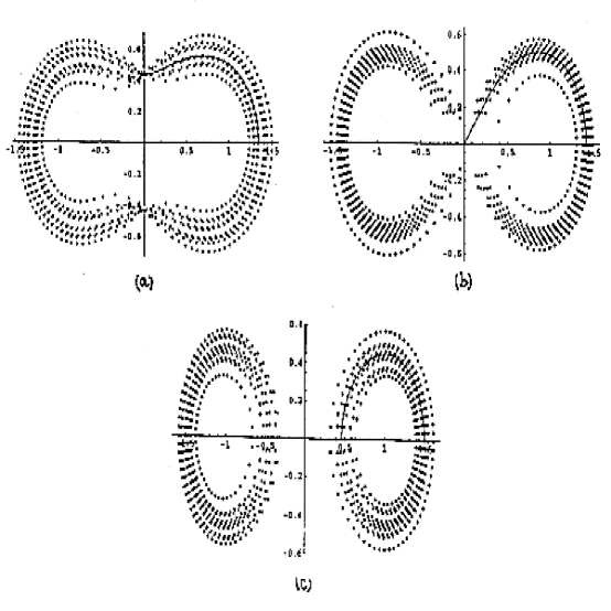
Figure 2: The spectrum of the Hamiltonian in Eq. (30). The site energies are taken from (31) for various values of $r$. Figures (a), (b) and (c) correspond to $r=0.9,1$ and $1.1$, respectively. The solid curve represents Eq. (37).

The width of the scatter of the numerical results around the analytical curve can be roughly estimated for any given $z_{0}$ on (37) by keepping (in addition to the leading term) all terms in the sum (34) with $|n-(N/2)|\leq N\epsilon(z_{0})$, where $\epsilon(z_{0})$ is determined by steepest descent. Then the branch singularities on the right hand side of (34) would have been bounded between the curves

$$(z^{2}-r^{2})\left({z+r\over z-r}\right)^{\pm\epsilon}=e^{i\theta}\,.$$ (38)

(Note added: In a forthcoming publication [10], it is shown that the width of the scatter vanishes as $N\rightarrow\infty$ and that the spectrum of the Hamiltonian in (30) is actually one dimensional.)

4 Many impurities and critical transitions

In this section we push the analysis of the previous section further and replace (31) by a generic probability distribution $P(w_{i})$.

Using the determinant (33) $\Delta(z)\equiv\left(\prod_{k=1}^{N}(z-w_{i})\right)-1$ we write the Green’s function for the “one way” Hamiltonian (30) as

$$G(z,z^{*})=\langle{1\over N}~{}{\partial_{z}\Delta(z)\over\Delta(z)}\rangle=\langle{1\over N}~{}\sum_{k=0}^{\infty}\sum_{i=1}^{N}{(\Delta(z))^{-k}\over z-w_{i}}\rangle\,.$$

Since each term in the previous equation factorizes, we finally arrive at the general formula

$$G(z,z^{*})=\langle{1\over z-w}\rangle-{1\over N}~{}{\partial\over\partial z}~{}\sum_{k=1}^{\infty}~{}{1\over k}\left[\langle\left({1\over z-w}\right)^{k}\rangle\right]^{N}\,,$$ (39)

where in each term we average over $w$ against the arbitrary distribution $P(w)$. A simple check reveals that (39) is consistent with (31) and (35). The averages $\langle\left(z-w\right)^{-k}\rangle$ may be obtained of course by deriving the generating function

$$g(z)=\langle{1\over z-w}\rangle\,.$$ (40)

It is worthwhile to mention here that a derivation of (39) by expanding in powers of the “one-way” hopping piece $H_{0}=\sum_{i}|i\rangle\langle i+1|$ in (30) has the nice feature that starting from any site $i$ on the chain, the terms that contribute to the trace (even without taking the average) are precisely those in which the particle hopped an integer number of complete revolutions around the chain (which is why the averages in (39) are all raised to the power $N$.) This observation may provide a physical explanation of why the determinant (33) is completely symmetric in the site energies $w_{i}$: the particle visits all sites equally as it hops, wherever the $w_{i}$’s are.

As a concrete application of (39) we now concentrate on the Lorentzian distribution (27) $P(w)=(\gamma/\pi)~{}(w^{2}+\gamma^{2})^{-1}$. We have $g(z,z^{*})=\left(z+i\gamma~{}{\rm sgn~{}(Im}~{}z)\right)^{-1}$ and obviously

$$\langle\left({1\over z-w}\right)^{k}\rangle=\left({1\over z+i\gamma~{}{\rm sgn~{}(Im}~{}z)}\right)^{k}=\left(g(z,z^{*})\right)^{k}\,.$$ (41)

Thus, using (39) we obtain the exact result

$$G(z,z^{*})={g(z,z^{*})\over 1-\left(g(z,z^{*})\right)^{N}}={\left(z+i\gamma~{}{\rm sgn~{}(Im}~{}z)\right)^{N-1}\over\left(z+i\gamma~{}{\rm sgn~{}(Im}~{}z)\right)^{N}-1}\,.$$ (42)

We would like now to calculate the density of eigenvalues. We first investigate $\rho(x,y)$ off the real axis. Using (25) ($\rho(x,y)=(1/\pi)~{}(\partial/\partial z^{*})~{}G(z,z^{*})$) we find

$$\rho(x,y) = {1\over\pi}~{}(z\pm i\gamma)^{N-1}~{}{\partial\over\partial z^{*}}~{}{1\over(z\pm i\gamma)^{N}-1}$$ (43)

$$= {1\over N}\sum_{k=0}^{N-1}\delta^{(2)}(z+i\gamma~{}{\rm sgn~{}(Im}~{}z)-\omega_{k})\,,$$

where $\omega_{k}=e^{2\pi ik/N}$, and $z\pm i\gamma$ in the first line of (43) correspond to $z$ being in the upper or lower half plane, respectively. The complex eigenvalues are thus equally spaced along the union of two arcs of a circle of radius one. The upper arc is that part of a semicircular arc of a unit circle (centered at the origin) that remains in the upper half plane after being pushed a distance $\gamma$ downward along the imaginary axis. (The lower arc is of course the mirror image of the upper arc.) Each of these arcs is thus of length ${\rm arc~{}cos}~{}(2\gamma^{2}-1)<\pi$ and carries $n_{{\rm arc}}=(N/2\pi)~{}{\rm arc~{}cos}~{}(2\gamma^{2}-1)~{}<~{}(N/2)$ eigenvalues. This means that the arcs exist only as long as $\gamma<\gamma_{c}=1$, which should be contrasted with the situation in (29). There, the single impurity does not perturb the unit circle, which persists for all values of $\gamma$.

The rest of the eigenvalues, which do not have space to live on the arcs, must have snapped onto the real axis and formed “wings”. The eigenvalue density along the real axis is generated when $\partial/\partial z^{*}$ hits the step-functions $\theta(\pm{\rm Im}~{}z)$ in (42) and we find that it is given by

$$\rho_{{\rm wing}}(x,y)={1\over\pi}~{}\delta(y)~{}{\rm Im}{(x-i\gamma)^{N-1}\over(x-i\gamma)^{N}-1}=-{\delta(y)\over\pi}~{}\mu^{N-1}~{}{\mu^{N}~{}{\rm sin}~{}\phi+{\rm sin}~{}(N-1)\phi\over\mu^{2N}-2\mu^{N}~{}{\rm cos}~{}N\phi+1}\,,$$ (44)

where we have defined $x-i\gamma\equiv\mu~{}e^{i\phi}$.

In the large $N$ limit (44) tends to a particularly simple form. It is clear that this form depends on whether $\mu~{}<~{}\mu_{c}=1$ or $\mu~{}>~{}\mu_{c}$. For $\mu~{}>~{}1$

$$\rho_{{\rm wing}}(x,y)=-{1\over\pi}~{}{{\rm sin}~{}\phi\over\mu}~{}\theta(\mu^{2}-1)~{}\delta(y)={\gamma\over\pi}~{}{1\over x^{2}+\gamma^{2}}~{}\theta(x^{2}+\gamma^{2}-1)~{}\delta(y)$$ (45)

(which again should be contrasted with the one impurity case (29),) while for $\mu~{}<~{}1$ $\rho_{\rm wing}=0$.

We thus see that for $\gamma~{}<~{}\gamma_{c}=1$, there are two wings that bifurcate from the arcs at $x=\pm x_{c}=\pm\sqrt{1-\gamma^{2}}$. Integrating over (45) we find that the fraction of eigenvalues that reside in the wings is $(n_{\rm wings}/N)=1-(2/\pi)~{}{\rm arc~{}cos}~{}\gamma=1-(1/\pi)~{}{\rm arc~{}cos}~{}(2\gamma^{2}-1)$, which together with the fraction of eigenvalues $2(n_{{\rm arc}}/N)=(1/\pi)~{}{\rm arc~{}cos}~{}(2\gamma^{2}-1)$ that reside in the arcs, sum up exactly to $1$. As $\gamma$ tends to $\gamma_{c}$, $x_{c}$ becomes smaller, and vanishes at $\gamma=\gamma_{c}$. At this point the two wings touch at the origin and the two arcs disappear completely.

As already mentioned, there is no critical $\gamma_{c}$ in the single impurity case, as perhaps might be expected. The many impurities case is dramatically different: the long tail of the Lorentz distribution can overwhelm the non-hermiticity for $\gamma~{}>~{}\gamma_{c}$, and the spectrum collapses to the real axis. We have carried out some numerical studies. For $\gamma$ away from $\gamma_{c}=1$, our analytic results fit the numerical data closely, but as $\gamma$ approaches $\gamma_{c}$, the statistical fluctuation between different realizations of $\{w_{i}\}$ becomes larger and larger (at $\gamma=0.9$ for example, for $N$ as large as 400.) It would be interesting to study the character of the transition in more detail.

It is perhaps worthwhile to remark that although in many discussions of disordered physics the gaussian distribution is the simplest to deal with, here it leads to a $g(z)$ not given by an elementary function.

Having derived a closed formula (Eq. (39)) for the Green’s function of the “one-way” model (30) (with pure clockwise hopping $H_{0}=\sum_{i}|i\rangle\langle i+1|$), we may now perturb it by adding a term $\Delta H=\tau\sum_{i}|i+1\rangle\langle i|$ (with $\tau$ small) which allows the particle to hop counter-clockwise. To first order in perturbation theory, the correction to the Green’s function (39) is now

$${\rm tr}~{}\left[{1\over z-w}~{}\left(H_{0}~{}{1\over z-w}\right)^{N+1}~{}\left(\Delta H~{}{1\over z-w}\right)\right]$$

which reflects the fact that the particle has completed one revolution around the chain by performing $N+1$ steps counter-clockwise and one step clockwise (which can occur anywhere along the chain.) It is thus possible to study the non-hermitean Hamiltonian (1) by perturbing both from the hermitean limit and the maximally non-hermitean limit.

In [5] we showed that by a hermitization method we can associate with every non-hermitean Hamiltonian $H$ a hermitean Hamiltonian ${\cal H}$. In particular, for the hopping Hamiltonians $H$ discussed in this paper, the Hamiltonian ${\cal H}$ involved the hopping of a particle with a binary internal state (call it an ”up” or a ”down” particle) such that as it hops it flips its internal state. Solving the Schrödinger equation associated with ${\cal H}$ amounts to a simultaneous solution of the Schrödinger equations associated with the two hermitean positive Hamiltonians $H_{1}=(z-H)(z-H)^{\dagger}$ and $H_{2}=(z-H)^{\dagger}(z-H)$. We see that for our “one-way” models $H_{1}$ and $H_{2}$ involve only nearest-neighbor hopping, while for the non-hermitean hopping models such as (1) or its generalizations described in Section (5), $H_{1}$ and $H_{2}$ involve next-nearest neighbor hopping

5 Continuum “One Way” models

The discrete “One Way” models of the two previous sections were solved exactly in the lagre $N$ limit. We now show that their continuum counterparts are also exactly solvable.

Starting with the continuum non-hermitean Schrödinger equation

$$H=-(1/m)[\partial_{x}+h]^{2}+W(x)$$ (46)

(with constant $h$), we reach the “One Way” limit by letting both $h$ and $m$ tend to infinity with a finite ratio $h/m$ (which we set to $1/2$.) In this limit, $H$ in (46) turns into the first order non-hermitean operator

$$H=-\partial_{x}+W(x)\,,$$ (47)

which is the desired continuum “One Way” model. Clearly, the spectrum of (46) may be solved explicitly for any $W(x)$, once the boundary conditions are specified. For example, if (47) is defined over $0\leq x\leq L$ with periodic boundary conditions, we have

$$\psi_{n}(x)~{} = {1\over\sqrt{L}}~{}{\rm exp}~{}(~{}\int\limits_{0}^{x}dyW(y)-E_{n}x)$$

$$\phi_{n}^{\dagger}(x) = {1\over\sqrt{L}}~{}{\rm exp}~{}(-\int\limits_{0}^{x}dyW(y)+E_{n}x)$$ (48)

where $\psi_{n}$ and $\phi_{n}$ are the eigenvectors on the right and on the left, respectively. Imposing the boundary conditions we find $E_{n}={1\over L}~{}\int\limits_{0}^{L}dyW(y)+{2i\pi n\over L}$ ($n$ being an integer.) Since we know the spectrum $\{E_{n}\}$ explicitly, we can now consider randomizing $W(x)$ in (47) and calculate any desired correlation function given any distribution of the random $W(x)$. For example, if $W(x)$ is drawn from the Gaussian distribution $P[W]=(1/Z)~{}{\rm exp}~{}[-(1/2g^{2})\int_{0}^{L}dxW^{2}(x)]$ we readily find that the averaged density of eigenvalues is

$$\rho({\rm Re}E,{\rm Im}E) \equiv \langle\sum_{n=-\infty}^{\infty}\delta\left({\rm Im}E-{2\pi n\over L}\right)\delta\left({\rm Re}E-{1\over L}\int_{0}^{L}dxW(x)\right)\rangle$$ (49)

$$= \sqrt{2\pi}(L/g)e^{-(L{\rm Re}E)^{2}/2g^{2}}\left[\sum_{n=-\infty}^{\infty}\delta\left({\rm Im}E-{2\pi n\over L}\right)\right]\,,$$

namely, each of the purely imaginary eigenvalues of $H_{0}=-\partial_{x}$, is smeared along the real axis by the fluctuations of the real potential $W(x)$. The spectrum is thus one dimensional, as in the discrete case.

6 Random hopping models and their mapping onto random walkers

In this section we study a different class of models, in which there is no site energy, but the hopping is random and non-hermitean. We consider the Schrödinger equation

$$E\psi_{j}=s_{j}^{*}\psi_{j+1}+t_{j-1}\psi_{j-1}$$ (50)

with the hopping amplitudes $s_{j}$ and $t_{j}$ generated randomly according to some prescription.

If the Hamiltonian is hermitean, then $s_{j}=t_{j}$. This hermitean problem was studied some twenty years ago by Eggarter and Riedinger [9]. They mapped the model onto a random walk problem and were able to show that all the states, except for the one at $E=0$, are localized, and furthermore, that the localization length diverges like $|{\rm log}E|$ as $E\rightarrow 0$. The existence of localized states is in accordance with the arguments of Anderson et al. [8]. In contrast, the appearance of an extended state at precisely $E=0$ is not generic and is due to the invariance of the spectrum under $E\rightarrow-E$ (as one can see by flipping the sign of $\psi_{i}$ for $i$ odd.) Thus, the extended state at $E=0$ is unstable under any perturbation that destroys this symmetry, such as adding random site energy.

Here we extend and generalize the analysis in [9] to the non-hermitean case. Our discussion below serves also as a review of [9], since obviously at any stage we can set $s_{j}$ equal to $t_{j}$. Dividing (50) by $\psi_{j}$ and defining $\Delta_{j}\equiv t_{j-1}\psi_{j-1}/\psi_{j}$ we obtain

$$\Delta_{j+1}={R_{j}\over E-\Delta_{j}}$$ (51)

where $R_{j}\equiv s_{j}^{*}t_{j}$. This equation is of course equivalent to Schrödinger’s equation (50) and allows us to solve for $\Delta_{j}$ iteratively and hence for the wave function $\psi$. For a closed chain the obvious boundary condition is $\Delta_{N+1}=\Delta_{1}$.

Performing a gauge transformation $\psi_{j}\rightarrow\lambda_{j}\psi_{j}$ we find that we can effectively transform $s_{j}^{*}\rightarrow(\lambda_{j+1}/\lambda_{j})s_{j}^{*}$ and $t_{j}\rightarrow(\lambda_{j}/\lambda_{j+1})t_{j}$. As perhaps expected, $R_{j}$ is invariant under this transformation. We see by these considerations that the open chain and the closed chain are quite different. For an open chain, we can always use this gauge freedom to set all the $t_{j}$ equal to $1$, say, with no loss of generality (which in the hermitean case would mean setting all the $s_{j}$ equal to $1$ as well, hence getting rid of randomness altogether.) On the other hand, for a closed chain with $N$ sites, we have the boundary condition $\psi_{N+1}=\psi_{1}$ and hence the constraint $\lambda_{N+1}=\lambda_{1}$. The gauge transformation is not in general useful.

We can of course invent a variety of models. Hatano and Nelson [3] considered $s_{j}^{*}=\tau_{j}~{}e^{\alpha}$ and $t_{j}=\tau_{j}~{}e^{-\alpha}$ where $\tau_{j}$ is taken from the flat distribution $P(\tau)={1\over 2\Delta}~{}\theta(\Delta^{2}-\tau^{2})$. We have studied one particularly simple model which we call the “clock model”, defined by setting $s_{j}$ and $t_{j}$ equal to random phases. In some sense, this model is particularly attractive, in that it includes no free parameters. Numerically, we found that the eigenvalues in the clock model are distributed (in what appears to be a uniform distribution) in a disk in the complex plane, centered at the origin and with radius approximately equal to $\pi/2$. The rotational invariance of the spectrum results from of our freedom to multiply the random Hamiltonian by an arbitrary overall phase.

Recall that the spectrum of any non-hermitean (or hermitean) hopping problem as defined in (50) is invariant under $E\rightarrow-E$. Furthermore, in the case of the clock model, the existence of an extended state at $E=0$ (provided $E=0$ is in the spectrum, which is always the case when the number of sites $N$ is odd) survives the non-hermiticity. This is so because the Schrödinger equation (50) for $E=0$ implies that $|\psi_{j+1}|=\Big{|}{t_{j-1}\over s_{j}^{*}}\psi_{j-1}\Big{|}=|\psi_{j-1}|$, and so this state is obviously extended. We expect the other states to be localized with an energy dependent localization length that diverges as $E\rightarrow 0$. These expectations are supported by the numerical studies we have done.

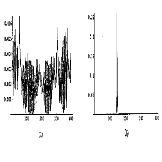
Figure 3: Two representative wave functions in one particular realization of the “clock model”. The wave function in Fig. (a) corresponds to the eigenvalue closest to the origin $E=0.04-0.14i$. It is extended and its participation ratio is 0.75. The wave function in (b) corresponds to the eigenvalue farthest from origin $E=-0.78+1.57i$. It is localized and its participation ratio is 0.01.

We would like now to discuss the divergence of the localization length as $E\rightarrow 0$. We thus focus on (50) for small $E$, that is $E$ small compared to a typical value of $\Delta_{j}$.

In the hermitean case, we have the important observation that $R_{j}=|t_{j}|^{2}$ is real and positive. Also, $E$ is real, and thus by (51) we can take $\Delta_{j}$ to be real (for an open chain, of course.) We see from (51) that for $E$ small compared to the typical scale of $\Delta$, the quantities $\Delta_{j}$ changes sign from site to site, and hence, as pointed out by Eggarter and Riedinger, it is convenient to iterate (51) twice and write

$$\Delta_{j+2}=\left({R_{j+1}\over R_{j}}\right)~{}\left[{1-{E\over\Delta_{j}}\over 1+{E(\Delta_{j}-E)\over R_{j}}}\right]~{}\Delta_{j}\,.$$ (52)

We can now define $z_{j}\equiv{\rm log}\Delta_{j}$ and interpret $z_{j}$ as the position of a random walker in the complex plane and $j$ as time. Taking the logarithm of (52) we obtain

$$z_{j+2}=z_{j}+{\rm log}~{}{R_{j+1}\over R_{j}}+{\rm log}~{}\left[{1-{E\over\Delta_{j}}\over 1+{E(\Delta_{j}-E)\over R_{j}}}\right]$$ (53)

defining the motion of the walker.

As noted above, for the hermitean case, $R_{j}$ is real and positive and thus the random walker stays on the real line. In particular, Eggarter and Riedlinger took $\langle{\rm log}~{}(R_{j+1}/R_{j})\rangle=0$ and defined $\sigma^{2}\equiv\langle\left({\rm log}~{}(R_{j+1}/R_{j})\right)^{2}\rangle$. They made the insightful observation that for $E\sim 0$ the last term in (53) (which would otherwise be too difficult to treat) could be taken into account effectively as boundary conditions set on the walker. Consider first the $-{\rm log}~{}\left[1+{E(\Delta_{j}-E)\over R_{j}}\right]$ part of that term. When $\Delta_{j}\sim(R_{j}/E)\sim$ a large positive number (we can always think of $\Delta_{j}$ as positive), the walker’s position on the real line (namely, $x_{j}={\rm log}~{}\Delta_{j}$) decreases rapidly. We can thus effectively replace the term under consideration by a reflecting wall located at ${\rm log}(R^{{}^{*}}/E)$ (which moves off to infinity as $E\rightarrow 0$), where $R^{{}^{*}}$ is a typical value of $R_{j}$. Consider now the remaining ${\rm log}~{}\left[1-{E\over\Delta_{j}}\right]$ part of that term. This part becomes important when $\Delta_{j}={\cal O}(E)$, at which point the sequence of $\Delta_{j}$ switches sign. We can thus think of a trap (or a “walker-eating monster”) located at $x\sim{\rm log}E$ (which wanders off to $-\infty$ as $E\rightarrow 0$.) Eggarter and Reidliger showed that the localization length can be related to the lifetime of the walker. In a numerical simulation we start with a walker being born at the wall ($x\sim+\infty$); typically he drifts rapidly towards $x\sim 0$, where he executes a random walk in his middle age, and as soon as he drifts into a substantially negative $x$ region, he rapidly approaches his death at $x\sim-\infty$.

It is perhaps satisfying that in going from the hermitean problem to the non-hermitean problem the random walker has escaped from the one dimensional world and wandered off into the complex plane. (Strictly speaking, due to the properties of the logarithm, the walker now lives on a cylinder with circumference $2\pi$.) The equation (53) describing the two dimensional walker is considerably more difficult to treat. One particularly simple case is given by the clock model in which the $\{R_{j}\}$ are pure random phases. Thus, separating $z_{j}=x_{j}+iy_{j}$, we see that as long as the term in square brackets in (53) is close to unity, the walker wanders in the $y$ direction, with its $x$ coordinate hardly changing.

We can estimate the localization length $L(E)$ rather crudely by noting that in the (supposedly) exponential tail of the localized wave function $|\Delta_{j}|\sim{\rm exp}~{}(\pm 1/L(E))$ and so $x_{j}\sim\pm 1/L(E)$. Thus we estimate $1/L(E)$ to be given by some average $x$ coordinate of the walker. In numerical studies, we observe that indeed, with the walker starting at $x=0$ he drifts into a random walk around some average $<x>$, (but then eventually wanders off.)

One message of this section is that random (non-hermitean) hopping models appear to be considerably more complicated than random (non-hermitean) site energy models. Indeed, let us mention that another interesting model we have studied, which we call a hopping “sign model”, is a restriction of the clock model, in which $s_{j}$ and $t_{j}$ are randomly (and independently) equal to $\pm 1$. This restriction destroys the rotational symmetry of the spectrum of the clock model, reducing it to a four fold symmetry, since eigenvalues must come in quadruplets $\pm E,\pm E^{*}$ (the Hamiltonian in this case is real and the symmetry of the spectrum under $E\rightarrow-E$ remains intact.) We obtained the density of eigenvalues numerically, and it exhibits a complicated interesting structure as shown in Fig.(4).

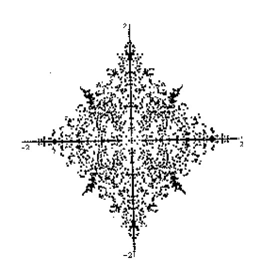
Figure 4: The spectrum of the hopping “sign model” for a chain with 400 sites. The amplitudes $s$ and $t$ take on values $\pm 1$ with equal probability.

It is an interesting challenge to calculate this structure analytically.

The hopping “sign model” is the strictest restriction of the “clock model”. It is thus interesting to investigate how the eigenvalue distribution of the “sign model” changes when we allow the hopping amplitudes to take on more values. For example, we studied numerically a $Z_{4}$ model in which $s_{j}$ and $t_{j}$ took on (independently) values from $\{\pm 1,\pm i\}$ with equal probability. We found that the intricate structure in Fig. (4) was largely washed out towards the uniform disk distribution of the “clock model”, with some residual fine structure.

At this point we mention a class of hopping models in which the $s$’s and $t$’s in (50) are taken from the same probability distribution $P(x)$ such that $x$ is always real and positive. Although the Hamiltonian $H$ is non-hermitean, the eigenvalues, that is, the solutions of det$(E-H)=0$, are all real for $N$ large. While surprising at first sight, this fact can be easily understood. The crucial observation is that $R_{j}=s_{j}t_{j}$ are all real and positive. For $N$ large, it does not make any difference whether the chain is closed or open as far as the eigenvalues are concerned, and so we can apply the transformation $s_{j}\rightarrow s_{j}^{{}^{\prime}}=(\lambda_{j+1}/\lambda_{j})s_{j}$ and $t_{j}\rightarrow t_{j}^{{}^{\prime}}=(\lambda_{j}/\lambda_{j+1})t_{j}$ mentioned earlier to make $s_{j}^{{}^{\prime}}=t_{j}^{{}^{\prime}}=\sqrt{R_{j}}$ (which is achieved by choosing $\lambda_{j+1}/\lambda_{j}=\sqrt{t_{j}/s_{j}}$.) Thus the model is effectively hermitean, that is, the eigenvalues (which are gauge invariant, of course) are real. Note that the “gauge” transformation just mentioned does not preserve the localization property of the wave function $\psi_{j}$. For instance, in numerical work, it is convenient to study the participation ratio, defined by $P(E)=1/(N\sum_{j}|\psi_{j}|^{4})$, such that $P\rightarrow 0$ for a localized state and $P\rightarrow 1$ for an extended state. Clearly, $P$ is not preserved by the “gauge” transformation in general, and therefore, say, a localized state may be gauged into an extended state (or vice-versa), unless the $\lambda_{j}$ are appropriately bounded as a function of the site index $j$. We thus have to do a case by case study of how the $\lambda_{j}$’s behave as a function of $j$ to infer the localization properties of the original wave functions from the gauge transformed wave functions of the effectively hermitean problem, which are of course all localized, as predicted by Anderson and others.

Note that the “sign model” mentioned in the previous paragraph and the hopping Hamiltonian $H_{0}$ in (2) both evade the defining conditions of this class of crypto-real models. An interesting question in mathematical physics is to calculate the fraction of eigenvalues escaping into the complex plane when the support of $P(x)$ includes negative values of $x$.

Finally, in connection with the question raised in the last paragraph, we mention here a class of hopping models in which the $s$’s and $t$’s in (50) are of the form $s_{j}=t+T_{j}$ and $t_{j}=t-T_{j}$, where the independent random amplitudes $\{T_{j}\}$ take values in the range $-T\leq T_{j}\leq T$ according to some, say, even probability distribution (this model is a one dimensional discrete analog of the two dimensional “model I” in [2].) For $t^{2}>T^{2}$ all $R_{j}$ are clearly positive with probability one, and thus the model is “crypto-real”. In general, the eigenvectors of the hermitean gauge transformed Hamiltonian would be all localized. Eigenvalues would start migrating into the compex plane only when $t^{2}<T^{2}$.

An amusing exception to the assertion that all states of the hermitean gauge transformed Hamiltonian are localized for $t^{2}>T^{2}$ is provided by the case in which the $\{T_{j}\}$ take on values $\pm T$ with equal probabilities. In this case $R_{j}\equiv R=t^{2}-T^{2}$ is actually deterministic and site independent and describes free hopping. Obviously, all states of the hermitean Hamiltonian are extended, regardless of the magnitude of disorder $T$. Clearly, $\sqrt{R}$, and thus all eigenvalues are real when $t^{2}>T^{2}$, and become pure imaginary for $t^{2}<T^{2}$. Thus, for this particular sign distribution, the answer to the question raised above is that for $t^{2}<T^{2}$ all eigenvalues escape into the complex plane (and onto the imaginary axis.)

7 Conclusion

We have studied localization and delocalization in a wide class of non-hermitean Hamiltonians. In various simplifying limits we were able to obtain analytic expressions. Our first model (10), while it involved only a single impurity, was able to capture the non-perturbative essence of the localization-delocalization transition. It was widely applicable to a generic $H_{0}$, in any spatial dimensions. For more explicit expressions, we had to invoke the maximally non-hermitean, or “one-way” limit, in which the spectrum of $H_{0}$ was a circle. (It is difficult to imagine that comparably simple expressions can be obtained when the spectrum of $H_{0}$ is an ellipse.) We were then able to analyze the problem of infinitely many impurities, one at each site. Results were given for several representative probability distributions $P(w)$ for the impurity potential energy $w$. We analyzed the phase transitions as parameters in $P(w)$ were varied.

We studied non-hermitean random hopping Hamiltonians. It has been known that the hermitean one dimensional random hopping problem can be mapped into a random walk problem on the real line. We found that in going from the hermitean to the non-hermitean problem, the random walker steps off the real axis and goes wandering off into the complex plane. We showed by numerical work that for the random phase or “clock model” the density of states appeared to be uniformly distributed over a disk, while in contrast for the “random sign” model the density of states showed a fascinatingly intricate structure.

The study of non-hermitean Hamiltonians opens up a rich area for exploration. We can immediately think of many questions to be answered. For instance, consider the many body problem (see also [3].) In the “one-way” model of (30) the many (non-interacting) fermion ground state will be described by a Slater determinant $\Psi\sim~{}{\rm det}_{i,j}[\psi_{i}(x_{j})]$ which in the large $N$ limit assumes the form $\prod_{i>j}~{}[e^{i\theta_{i}}-e^{i\theta_{j}}]$. The question arises, even before we consider impurities, on what is meant by the lowest energy state of $H_{0}$. In other words, as we fill the system with non-interacting fermions, how do we order the energy levels if they are arranged in a circle? These questions may perhaps be answered by coupling the system to some agent (such as a radiation field or a heat bath) which can exchange energy with the many body system.

As another set of questions, we can ask how a non-hermitean many body system can be second quantized? What are some of the properties of a non-hermitean quantum field theory, such as a gauge theory in which the gauge potential $A_{\mu}$ is non-hermitean? In a relativistic theory, if the Hamiltonian becomes non-hermitean, does Poincaré invariance imply that its other nine generators should become non-hermitean as well?

Acknowledgements    One of us (A. Zee) thanks D. Nelson for interesting him in this problem and for continuing discussions, P. W. Anderson and M. P. A. Fisher for discussions about localization, and J. Chalker for suggesting that we examine the Lorentz distribution. We also thank J. Miller for calling our attention to [2]. Part of this work was done at the Institute for Advanced Study where he was the Dyson Distinguished Visiting Professor and he thanks the Dyson Fund for its support. This work was partly supported by the National Science Foundation under Grant No. PHY89-04035.

Appendix : Non-hermitean perturbation theory

It is of course a trivial exercise to treat the model in (1) perturbatively in the strength of the random impurity. Denote the eigenvalues of $H_{0}$ and $H$ by $\{E_{\mu}\}$ and $\{E_{\mu}(w)\}$ respectively. Write $H_{0}=S^{-1}ES$ with $E$ the diagonal matrix with elements $\{E_{\mu}\}$ (and thus the columns of $S^{-1}$ and the rows of $S$ are the right and left eigenvectors of $H_{0}$, respectively.) Define

$$E_{\mu}(w)=E_{\mu}+\sum_{i}w_{i}\,E_{\mu i}+\sum_{i,j}w_{i}w_{j}\,E_{\mu ij}+\cdots$$ (A.1)

Then by simple arithmetic we obtain

$$E_{\mu i} = S^{-1}_{i\mu}S_{\mu i}$$

$$E_{\mu ij} = \sum_{\nu\neq\mu}{S^{-1}_{i\mu}S_{\mu j}S^{-1}_{j\nu}S_{\nu i}\over E_{\mu}-E_{\nu}}$$ (A.2)

and so on. It follows that the averaged density of eigenvalues of $H$ is given to ${\cal O}(w^{2})$ by

$$\rho(x,y) = \rho_{0}(x,y)+{w^{2}\over N}\sum_{\mu}\left\{\left[\delta^{\prime}(x-{\rm Re}~{}E_{\mu})~{}\delta^{\prime}(y-{\rm Im}~{}E_{\mu})~{}\sum_{i}{\rm Re}~{}E_{\mu i}~{}{\rm Im}~{}E_{\mu i}\right]\right.$$

$$- \left.{1\over 2}\left\{2\delta^{\prime}(x-{\rm Re}~{}E_{\mu})~{}\delta(y-{\rm Im}~{}E_{\mu})~{}\sum_{i}{\rm Re}~{}E_{\mu ii}\right.\right.$$

$$- \left.\left.\delta^{\prime\prime}(x-{\rm Re}~{}E_{\mu})~{}\delta(y-{\rm Im}~{}E_{\mu})~{}\sum_{i}({\rm Re}~{}E_{\mu i})^{2}+[x\leftrightarrow y,\,{\rm Re}\leftrightarrow{\rm Im}]\right\}\right\}$$

where we have used only $\langle w_{i}w_{j}\rangle=w^{2}\delta_{ij}$. The result (7) holds for all $H_{0}$ (and for finite $N$.) For the specific $H_{0}$ in (2) and in the large $N$ limit there are drastic simplifications. We have $E_{\mu i}=1/N$ and so ${\rm Im~{}}E_{\mu_{i}}=0$ and $\sum_{i}\left({\rm Re~{}}E_{\mu i}\right)^{2}=1/N$. Thus the only non-trivial quantity that comes in is

$$\sum_{i}E_{\mu ii}={1\over Nt}\sum_{\nu\neq\mu}{1\over{\rm cosh}~{}(h+ik(\mu))-{\rm cosh~{}}(h+ik(\nu))}$$ (A.4)

where $k(\mu)=2\pi\mu/N,\quad\mu=0,1,\cdots N-1$. The expression (7) simplifies to

$$\rho(x,y)={1\over N}\sum_{\mu}\delta(x-{\rm Re~{}}E_{\mu}-w^{2}\sum_{i}{\rm Re~{}}E_{\mu ii})\delta(y-{\rm Im~{}}E_{\mu}-w^{2}\sum_{i}{\rm Im~{}}E_{\mu ii})\,.$$ (A.5)

The sum in (A.5) can be converted to an integral and evaluated in principle. For the “one way” model described in the text the integral is particularly simple and we obtain

$$\rho(x,y)=\int\limits_{0}^{2\pi}{d\theta\over 2\pi}~{}\delta\left(x-(1+{w^{2}\over 2}){\rm cos~{}}\theta\right)~{}\delta\left(y-(1-{w^{2}\over 2}){\rm sin~{}}\theta\right)\,.$$ (A.6)

To this order in $w$, the circle has been turned into an ellipse. Of course, we do not see any trace of the wings in perturbation theory.

References

-
[1]
F. Haake, F. Izrailev, N. Lehmann, D. Saher and H. J. Sommers, Zeit. Phys. B 88 (1992) 359.
H. J. Sommers, A. Crisanti, H. Sompolinsky and Y. Stein, Phys. Rev. Lett. 60 (1988) 1895.
M. A. Stephanov, Phys. Rev. Lett. 76 (1996) 4472 .
R. A. Janik, M. A. Nowak, G. Papp and I. Zahed, preprints cond-mat/9612240, hep-ph/9606329.
R. A. Janik, M. A. Nowak, G. Papp, J. Wambach and I. Zahed, preprint hep-ph/9609491.
E. Gudowska-Nowak, G. Papp and J. Brickmann, preprint cond-mat/9701187.
Y. V. Fyodorov, B. A. Khoruzhenko and H. J. Sommers, Phys. Lett. A 226 (1997) 46, Phys. Rev. Lett. 79 (1997) 557; B. A. Khoruzhenko Jour. Phys. A. (Math. Gen.) 29 (1996) L165.
M. A. Halasz, A. D. Jackson and J. J. M. Verbaarschot, preprints, hep-lat/9703006, hep-lat/9704007.
J. Feinberg and A. Zee, preprint cond-mat/9704191 (Nucl. Phys. B, to appear.)
J. T. Chalker and Z. Jane Wang, preprint cond-mat/9704198. - [2] J. Miller and Z. Jane Wang, Phys. Rev. Lett. 76 (1996) 1461.
- [3] N. Hatano and D. R. Nelson, Phys. Rev. Lett. 77 (1997) 570; for a more detailed discussion see N. Hatano and D. R. Nelson, preprint cond-mat/9705290.
- [4] K. B. Efetov, preprint cond-mat/9702091.
- [5] J. Feinberg and A. Zee, preprint cond-mat/9703087 (Nucl. Phys. B, to appear.)
- [6] R. A. Janik, M. A. Nowak, G. Papp J. Wambach and I. Zahed, preprint cond-mat/9705098.
- [7] P. W. Brouwer, P. G. Silvestrov and C. W. J. Beenakker, preprint cond-mat/9705186.
-
[8]
P. W. Anderson, Phys. Rev. 109 (1958) 1492;
R. Abou-Chacra, P. W. Anderson and D. J. Thouless, Jour. Phys. C6 (1973) 1734; R. Abou-Chacra and D. J. Thouless, Jour. Phys. C7 (1974) 65;
E. Abrahams, P. W. Anderson, D. C. Licciardelo and T. V. Ramakrishnan, Phys. Rev. Lett. 42 (1979) 673;
E. Abrahams, P. W. Anderson, D. S. Fisher and D. J. Thouless, Phys. Rev. B 22 (1980) 3519; P. W. Anderson, Phys. Rev. B 23 (1981) 4828. - [9] T. P. Eggarter and R. Riedinger, Phys. Rev. B 18 (1978) 569.
- [10] E. Brèzin and A. Zee, preprint cond-mat/9708029.