Continuous renormalization for fermions
and Fermi liquid theory

I derive a Wick ordered continuous renormalization group equation for fermion systems and show that a determinant bound applies directly to this equation. This removes factorials in the recursive equation for the Green functions, and thus improves the combinatorial behaviour. The form of the equation is also ideal for the investigation of many-fermion systems, where the propagator is singular on a surface. For these systems, I define a criterion for Fermi liquid behaviour which applies at positive temperatures. As a first step towards establishing such behaviour in $d\geq 2$, I prove basic regularity properties of the interacting Fermi surface to all orders in a skeleton expansion. The proof is a considerable simplification of previous ones.

1 Introduction

In this paper, I begin a study of fermionic quantum field theory by a continuous Wick ordered renormalization group equation (RGE). As an example, I take the standard many-fermion system of solid state quantum field theory, but the method applies to general fermionic models with short-range interactions. I show that a determinant of propagators appears in the RGE and I use a determinant bound to prove that a factorial which would appear in bosonic theories is removed from the recursion for the fermionic Green functions. This may lead to convergence of perturbation theory in the absence of relevant couplings, but I do not address the convergence problem, which is related to the solution of a particular combinatorial recursion, in this paper. A short account of this work has appeared in [13].

Continuous RGEs were invented by Wegner [1] and Wilson [2]. Polchinski [3] found a beautiful way to use them for a proof of perturbative renormalizability of $\phi^{4}$ theory. His method was simplified in [5], and extended to composite operator renormalization and to gauge theories by Keller and Kopper [6]. Keller [7] also proved local Borel summability. While equivalent to the Gallavotti-Nicolò [8, 9, 10] method, the continuous RGE is much simpler technically. An application of continuous RG methods to nonperturbative bosonic problems [11, 12] requires many new ideas and a combination with cluster expansion techniques, to control the combinatorics. It is one of the points of this paper that for fermions, the straightforward adaption of the method yields a determinant bound which improves the combinatorics of fermionic theories as compared to bosonic ones, and may lead to nonperturbative bounds. The determinant structure is not visible in the form of the flow equation used in [3, 5, 6], because the flow equation in that form is a one-loop equation which has too little structure. A key ingredient for the present analysis is Wick ordering, which was first used in the context of continuous RGEs for scalar field theories by Wieczerkowski [4]. I show that for fermions, the Wick ordered RGE contains a determinant of propagators to which a Gram inequality applies directly. A closer look at the way the Feynman graph expansion is generated by the RGE shows that the sign cancellations bring the combinatorial factors for fermions nearer to that of a planar field theory. This reduction does, however, not lead to a planar field theory in the strict sense because of certain binomial factors in the recursion.

The direct application of the determinant bound shown here requires the interaction between the fermions to be short-range. This prevents a straightforward application to systems with abelian gauge fields by simply integrating over the gauge fields. One model to which the method applies directly is the Gross-Neveu model (which has been constructed rigorously [14, 15]). I show here only the most basic power counting bounds by leaving out all relevant and marginal couplings, but it is possible to take them into account by renormalization.

A class of physically realistic models with a short-range interaction is that of nonrelativistic many-fermion models. In these models, there is a significant complication of the analysis because the singularity of the fermion propagator in momentum space is not at a point, but instead on the Fermi surface, which is a $(d-1)$-dimensional subset of momentum space. Only in one dimension, the singularity is pointlike – the ‘surface’ becomes a point.

The interest in these models has resurged recently because of the discovery of high-temperature superconductivity. Before that it was taken for granted that Fermi liquid (FL) behaviour holds in all dimensions $d\geq 2$, and Luttinger liquid behaviour in one dimension (the latter has been proven [16, 17, 18]). At certain doping values, however, strong deviations from FL behaviour are seen in the high-$T_{c}$ materials. The discussion following these discoveries revealed that the former arguments for FL behaviour contained logical gaps. Like [19, 20, 21, 22, 23, 24, 25], the present work is not aimed at an understanding of these deviations, but at the more modest goal of determining first under which conditions FL behaviour occurs.

Before doing so, it is necessary to give a definition of what would constitute FL behaviour. At zero temperature, the noninteracting Fermi gas has a discontinuity in the occupation number density; this is also a property one would require of a zero temperature FL. This discontinuity is absent for Luttinger liquids. It is, however, not sufficient for FL behaviour because there is a one-dimensional model which has both such a discontinuity and some Luttinger liquid features in the spectral density [26]. Moreover, in the standard models of many-fermion systems such a step never occurs because superconductivity sets in below a critical temperature, and it smoothes out the step in the zero-temperature Fermi distribution. It is thus desirable to give a definition of FL behaviour at temperatures above the critical temperature for superconductivity. This is not at all straightforward because there is no clean characterization of FL behaviour at a fixed temperature. I propose to look at a whole range of temperatures and values of the coupling constant to bring out the characteristic features of a FL.

I define an equilibrium Fermi liquid as a system in which the perturbation expansion in the coupling constant $\lambda$ converges for the skeleton Green functions in the region $|\lambda|\log\beta$ small enough (here $\beta$ is the inverse temperature) and where the self-energy fulfils certain regularity conditions. The skeleton Green functions are defined in detail in Section 6; in them, self-energy insertions are left out, so that the Fermi surface stays fixed. I discuss in Section 7 how they are related to the exact Green functions. The logarithmic dependence of the radius of convergence on $\beta$ comes from the Cooper instability; the difference between Fermi liquids and Luttinger liquids is in the regularity properties of the self-energy. This is discussed in detail in Section 2.6.

The goal is to show that the standard many-fermion systems are Fermi liquids in that sense. A proof of this requires a combination of the regularity techniques of [21, 22, 23] for renormalization with the sector technique of [20] in the determinant bound (see Section 2.6 for further discussion). I do not give a complete proof in this paper but only a part of it, by showing a determinant bound and some of the required regularity properties of the selfenergy in perturbation theory. The hope is that the determinant bound will lead to convergence, so that the method developed here, which is somewhat simpler than e.g. the one in [20], will work nonperturbatively. A different representation for fermionic Green functions that provides a simplification and leads to nonperturbative bounds is given in [27].

In Section 2, I review the Grassmann integral for many-fermion systems briefly, to give a self-contained motivation for the study of such systems, and to fix notation. The Fermi liquid criterion is formulated in Section 2.6. Section 3 contains the general renormalization group equation and the determinant formula Eq. $(\ref{Qrmtdef})$. Section 4 contains the determinant bound and an application to systems where the propagator has point singularities. In Section 5, I show the existence of the thermodynamic limit for the many-fermion system in perturbation theory. In Section 6, I prove bounds on the skeleton self-energy that are needed to renormalize the full theory in perturbation theory. Again, the RGE in the form of [3, 5, 6] would not be very convenient for this because it is a one-loop equation, whereas the crucial effects for regularity all start at two loops. They can be seen in a simple way in the Wick ordered RGE. Details about Wick ordering and the derivation of the determinant formula Eq. $(\ref{Qrmtdef})$ are deferred to the Appendix.

Acknowledgement: I thank Volker Bach, Walter Metzner, Erhard Seiler, and Christian Wieczerkowski for discussions. I also thank Christian Lang for his hospitality at a very pleasant visit to the University of Graz, where this work was started.

2 Many-fermion systems

The model is defined on a spatial lattice with spacing $\varepsilon$. Continuum models are obtained in the limit $\varepsilon\to 0$; lattice models, such as the Hubbard model, are obtained by fixing $\varepsilon$.

Let $d\geq 2$ be the spatial dimension, $\varepsilon>0$, $L\in{\mathbb{R}}$ be such that $\frac{L}{2\varepsilon}\in{\mathbb{N}}$, and let ${\mathbb{G}}$ be any lattice of maximal rank in ${\mathbb{R}}^{d}$, e.g., ${\mathbb{G}}={\mathbb{Z}}^{d}$. Let ${\mathbb{L}}$ be the torus ${\mathbb{L}}=\varepsilon{\mathbb{G}}/L{\mathbb{G}}$. The number of points of this lattice is $|{\mathbb{L}}|=(\frac{L}{\varepsilon})^{d}$. Let $\int_{\mathbb{L}}d{\bf x}\;F({\bf x})=\varepsilon^{d}\sum_{{\bf x}\in{\mathbb{L}}}F({\bf x})$ and $\delta_{\mathbb{L}}({\bf x},{\bf x}^{\prime})=\varepsilon^{-d}\delta_{{\bf x},{\bf x}^{\prime}}$.

Let ${\cal F}_{\mathbb{L}}$ be the Fock space generated by the spin one half fermion operators satisfying the canonical anticommutation relations [28], i.e. for all ${\bf x},{\bf x}^{\prime}\in{\mathbb{L}}$,

$$c_{\alpha}({\bf x})c^{+}_{\alpha^{\prime}}({\bf x}^{\prime})+c^{+}_{\alpha^{\prime}}({\bf x}^{\prime})c_{\alpha}({\bf x})=\delta_{\alpha\alpha^{\prime}}\;\delta_{\mathbb{L}}({\bf x},{\bf x}^{\prime}).$$ (1)

Here $\alpha\in\{-1,1\}$ is the spin of the fermion in units of $\frac{\hbar}{2}$. The free part of the Hamiltonian $H_{\mathbb{L}}(c,c^{+})=H_{0}+\lambda V$ is

$$H_{0}=-\sum\limits_{\alpha\in\{-1,1\}}\int\limits_{{\mathbb{L}}}d{\bf x}\;\int\limits_{{\mathbb{L}}}d{\bf y}\;T({\bf x},{\bf y})\;c^{+}_{\alpha}({\bf x})c_{\alpha}({\bf y}).$$ (2)

For a one-band model on a lattice with fixed spacing $\varepsilon$, $T({\bf x},{\bf y})=t_{{\bf x}-{\bf y}}=t_{{\bf y}-{\bf x}}$ describes hopping from a site ${\bf y}$ to another site ${\bf x}$ with an amplitude $t_{{\bf x}-{\bf y}}=t_{{\bf y}-{\bf x}}$.

The interaction is multiplied by a small coupling constant $\lambda$; I assume it to be a normal ordered density-density interaction

$$V(c,c^{+})=-\int\limits_{{\mathbb{L}}}d{\bf x}\;\int\limits_{{\mathbb{L}}}d{\bf y}\;\sum\limits_{\alpha,\sigma\in\{-1,1\}}v({\bf x}-{\bf y})c^{+}_{\alpha}({\bf x})c^{+}_{\sigma}({\bf y})c_{\alpha}({\bf x})c_{\sigma}({\bf y})$$ (3)

In other words, it is a special type of a four-fermion interaction.

For instance, the simplest Hubbard model is given by $\lambda=\frac{U}{2}$ where $U$ is the usual Hubbard-$U$, and by $v({\bf x}-{\bf y})=\delta_{\mathbb{L}}({\bf x},{\bf y})$, and the hopping term is $t_{{\bf x}-{\bf y}}=t$ if $|{{\bf x}-{\bf y}}|=1$ and zero otherwise, where $t$ is the hopping parameter.

At temperature $T$ and chemical potential $\mu$, the grand canonical partition function is given by $Z_{\mathbb{L}}=\mbox{ tr}_{{\cal F}_{\mathbb{L}}}\left({\rm e}^{-\beta(H_{\mathbb{L}}-\mu N_{\mathbb{L}})}\right)$ with $N_{\mathbb{L}}=\int_{\mathbb{L}}d{\bf x}\;n({\bf x})$, and $\beta=\frac{1}{k_{B}T}$. Observables are given by expectation values of functions, mainly polynomials, of the $c$ and $c^{+}$,

$$\langle{\cal O}\rangle_{\mathbb{L}}=\frac{1}{Z_{\mathbb{L}}}\mbox{ tr}\left({\rm e}^{-\beta(H_{\mathbb{L}}-\mu N_{\mathbb{L}})}{\cal O}(c,c^{+})\right)$$ (4)

A basic question is whether the expected values of observables have a finite thermodynamic limit and whether an expansion in $\lambda$ can be used to get their behaviour at small or zero temperature $T$. For instance, one would like to expand the two-point function $\langle c^{+}({\bf x})c({\bf y})\rangle_{\mathbb{L}}=\sum_{r=0}^{\infty}\lambda^{r}G_{2,r}^{L,\varepsilon}({\bf x},{\bf y})$. It is by now well-known that the result of a naive expansion ${\rm e}^{-\lambda V}$ in powers of $\lambda$ is that at $T=0$, $\lim_{L\to\infty}G_{2,r}^{L,\varepsilon}=\infty$ for all $r\geq 3$ (see, e.g., [19, 21]). At positive temperature $T$, this unrenormalized expansion converges for $|\lambda|\leq\hbox{ \rm const }T^{d}$; see Section 4. To get a better $T$-dependence of the radius of convergence, one has to renormalize. Because of the BCS instability, the best one can hope for in general is a bound $|\lambda|\log{\textstyle\frac{1}{T}}<\hbox{ \rm const }$ for the region of convergence. This is part of the Fermi liquid criterion formulated below.

2.1 Grassmann integral representation

The standard Grassmann integral representation is obtained by applying the Lie product formula

$${\rm e}^{-\beta(H_{\mathbb{L}}-\mu N_{\mathbb{L}})}=\lim\limits_{n_{\tau}\to\infty}\left({\rm e}^{-\varepsilon_{\tau}(H_{0}-\mu N_{\mathbb{L}})}\;{\rm e}^{-\varepsilon_{\tau}\lambda V}\right)^{n_{\tau}}$$ (5)

to the trace for $Z_{\Lambda}$ and $\langle{\cal O}\rangle$. The spacing in imaginary-time direction is $\varepsilon_{\tau}=\frac{\beta}{n_{\tau}}$. The limit exists in operator norm because on the finite lattice ${\mathbb{L}}$, all operators are just finite-dimensional matrices.

Inserting the orthonormal basis of ${\cal F}_{\mathbb{L}}$ between the factors in Eq. $(\ref{Trotto})$ and rearranging, I get $Z_{\mathbb{L}}=\lim_{n_{\tau}\to\infty}Z_{{\mathbb{L}},n_{\tau}}$, where $Z_{{\mathbb{L}},n_{\tau}}$ is given by a finite-dimensional Grassmann integral, as follows. Let $n_{\tau}$ be even and ${\mathbb{T}}=\{\tau=n\varepsilon_{\tau}:\;n\in{\mathbb{Z}},\;-\frac{n_{\tau}}{2}\leq n<\frac{n_{\tau}}{2}\}$, let $\Lambda={\mathbb{T}}\times{\mathbb{L}}$, and ${\cal A}$ be the Grassmann algebra generated by $\psi_{\sigma}(x)$, ${\bar{\psi}}_{\sigma}(x)$, with $\sigma\in\{1,-1\}$ and $x=(\tau,{\bf x})\in\Lambda$. Fix some ordering on $\Lambda$ and denote the usual Grassmann measure [29, 30] by $D_{\Lambda}\psi D_{\Lambda}{\bar{\psi}}=\prod_{x,\sigma}d\psi_{\sigma}(x)\;d{\bar{\psi}}_{\sigma}(x)$. Then Eq. $(\ref{Trotto})$ implies $Z_{{\mathbb{L}},n_{\tau}}={\cal N}_{\Lambda}\int D_{\Lambda}\psi D_{\Lambda}{\bar{\psi}}\;{\rm e}^{-S_{\Lambda}(\psi,{\bar{\psi}})}$ where ${\cal N}_{\Lambda}$ is a normalization factor that depends on $\varepsilon,L$, and $n_{\tau}$, and where

$$S_{\Lambda}(\psi,{\bar{\psi}})=\int_{\mathbb{T}}d\tau\left(\sum\limits_{\sigma}\int\limits_{\mathbb{L}}d{\bf x}\;{\bar{\psi}}_{\sigma}(\tau,{\bf x})\partial_{\tau}\psi_{\sigma}(\tau,{\bf x})\;-\;H_{\Lambda}(\psi(\tau),{\bar{\psi}}(\tau))\right)$$ (6)

Here I have used the notations $\psi(\tau)({\bf x})=\psi(\tau,{\bf x})$, $\int_{\mathbb{T}}d\tau F(\tau)=\varepsilon_{\tau}\sum_{\tau\in{\mathbb{T}}}F(\tau)$, and $\partial_{\tau}\psi(\tau)=\varepsilon_{\tau}^{-1}(\psi_{\sigma}(\tau+\varepsilon_{\tau})-\psi_{\sigma}(\tau))$, and the sum over $\tau$ runs over ${\mathbb{T}}$, with antiperiodic boundary conditions [31]. For $n_{\tau}<\infty$ and $L<\infty$, this is a finite-dimensional Grassmann integral. The limit $n_{\tau}\to\infty$, and afterwards $L\to\infty$, will be taken only for the effective action. No infinite-dimensional Grassmann integration will be required.

To do the Fourier transformation, it will be convenient to deal with periodic functions defined on an interval of double length in $\tau$, and to impose the antiperiodicity as an antisymmetry condition: let ${\mathbb{T}}_{2}=\varepsilon_{\tau}{\mathbb{Z}}/2\beta{\mathbb{Z}}$, in other words, ${\mathbb{T}}_{2}=\{\tau\in\varepsilon_{\tau}{\mathbb{Z}}:-\beta\leq\tau<\beta\}$ with periodic boundary conditions. Thus the fields $\psi$ and ${\bar{\psi}}$ are periodic with respect to translations of $\tau$ by $2\beta$, and antiperiodicity with respect to translations by $\beta$ is imposed by setting

$${\mathop{\psi}\limits^{\scriptscriptstyle{(-)}}}(\tau+\beta,{\bf x})=-{\mathop{\psi}\limits^{\scriptscriptstyle{(-)}}}(\tau,{\bf x})$$ (7)

for all $x\in\Lambda$. With the further notation $\int_{\Lambda}dx\;F(x)=\int_{{\mathbb{T}}}d\tau\int_{\mathbb{L}}d{\bf x}\;F(\tau,{\bf x})$, and $\delta_{\Lambda}(x,x^{\prime})={\varepsilon_{\tau}}^{-1}\varepsilon^{-d}\delta_{\tau,\tau^{\prime}}\delta_{{\bf x},{\bf x}^{\prime}}$, the action is $S(\psi,{\bar{\psi}})=S_{2}(\psi,{\bar{\psi}})+\lambda S_{4}(\psi,{\bar{\psi}})$ where

$$S_{2}(\psi,{\bar{\psi}})=\sum\limits_{\sigma,\sigma^{\prime}}\int\limits_{\Lambda}dx\;\int\limits_{\Lambda}dx^{\prime}\;{\bar{\psi}}_{\sigma}(x)\;a(x,\sigma,x^{\prime},\sigma^{\prime})\psi_{\sigma^{\prime}}(x^{\prime})$$ (8)

with

$$a(x,\sigma,x^{\prime},\sigma^{\prime})=\delta_{\sigma\sigma^{\prime}}\left((\partial_{\tau}+\mu)\delta_{\Lambda}(x,x^{\prime})-T({\bf x},{\bf x}^{\prime})\delta_{{\mathbb{T}}_{2}}(\tau,\tau^{\prime})\right)$$ (9)

and

$$S_{4}(\psi,{\bar{\psi}})=\sum\limits_{\sigma,\sigma^{\prime}}\int\limits_{\Lambda}dx\;\int\limits_{\Lambda}dx^{\prime}\;{\bar{\psi}}_{\sigma}(x)\psi_{\sigma}(x)v(\tau,{\bf x},\tau^{\prime},{\bf x}^{\prime}){\bar{\psi}}_{\sigma^{\prime}}(x^{\prime})\psi_{\sigma^{\prime}}(x^{\prime})$$ (10)

with $v(\tau,{\bf x},\tau^{\prime},{\bf x}^{\prime})=\delta_{{\mathbb{T}}_{2}}(\tau,\tau^{\prime})v({\bf x}-{\bf x}^{\prime})$. For the present work, the interaction does not have to be instantaneous. Retardation effects, like from phonons, are allowed. That is, $v(\tau,{\bf x},\tau^{\prime},{\bf x}^{\prime})$ may have a dependence on $\tau$ and need not be local in $\tau$.

The operator $a$ appearing in $S_{2}$ is invertible because the antiperiodicity condition removes the zero modes of the discretized time derivative. In other words, the Matsubara frequencies for fermions are nonzero at positive temperature (this will become explicit in the next section).

2.2 The propagator in Fourier space

Fourier transformation with the antiperiodicity conditions Eq. $(\ref{psanti})$ is described in Appendix A. The Fourier transforms of $\psi$ and ${\bar{\psi}}$ are

$$\hat{\mathop{\psi_{\sigma}}\limits^{{}_{(-)}}}(p)=\int\limits_{\Lambda}dx\;{\rm e}^{-{\rm i}px}\;{\mathop{\psi_{\sigma}}\limits^{{}_{(-)}}}(x)$$ (11)

where, for $p=(\omega,{\bf p})$ and $x=(\tau,{\bf x})$, $px=\omega\tau+{\bf p}{\bf x}$. If ${\mathbb{L}}^{*}$ is the dual lattice to ${\mathbb{L}}$, the momentum $p$ is in ${\Lambda^{*}}={\mathbb{M}}_{n_{\tau}}\times{\mathbb{L}}^{*}$, where

$${\mathbb{M}}_{n_{\tau}}=\{\omega_{n}=\frac{\pi}{\beta}(2n+1):\;n\in{\mathbb{Z}},\;-\frac{n_{\tau}}{2}\leq n<\frac{n_{\tau}}{2}\}$$ (12)

is the set of Matsubara frequencies $\omega_{n}$. With the notation $\int_{{\Lambda^{*}}}dp\;F(p)=\frac{1}{\beta}\sum_{\omega\in{\mathbb{M}}_{n_{\tau}}}\;\int_{{\mathbb{L}}^{*}}d{\bf p}\;F(\omega,{\bf p})$, where $\int_{{\mathbb{L}}^{*}}d{\bf p}=L^{-d}\sum_{{\bf p}\in{\mathbb{L}}^{*}}$, the inverse Fourier transform is $\psi_{\sigma}(x)=\int_{{\Lambda^{*}}}dx\;{\rm e}^{{\rm i}px}\;\hat{\psi}_{\sigma}(p)$. The Fourier transform of the hopping term is $\hat{T}({\bf p},{\bf q})=\delta_{{\mathbb{L}}^{*}}({\bf p}+{\bf q},0)\tilde{T}({\bf q})$, with $\tilde{T}({\bf q})=\int\limits_{{\mathbb{L}}}d{\bf z}\;{\rm e}^{{\rm i}{\bf q}{\bf z}}t_{\bf z}$. Denoting

$$E({\bf p})=\tilde{T}({\bf p})-\mu,$$ (13)

where $\mu$ is the chemical potential,

$$\widehat{\omega}=\frac{1}{{\rm i}\varepsilon_{\tau}}\left({\rm e}^{{\rm i}\varepsilon_{\tau}\omega}-1\right),$$ (14)

and $\delta_{{\Lambda^{*}}}(p+p^{\prime},0)=\delta_{{\mathbb{L}}}({\bf p}+{\bf p}^{\prime},0)\;{\varepsilon_{\tau}}^{-1}\delta_{-\omega,\omega^{\prime}}$, the Fourier transform of the operator $a$ in the quadratic part of the action is

$$\hat{a}(p,\sigma,p^{\prime},\sigma^{\prime})=\delta_{\Lambda}(p+p^{\prime},0)\delta_{\sigma\sigma^{\prime}}\;\left({\rm i}\widehat{\omega^{\prime}}-E({\bf p}^{\prime})\right)$$ (15)

In other words, the matrix with entries $\hat{a}(p,\sigma,-p^{\prime},\sigma^{\prime})$ is diagonal, and for temperature $T={\textstyle\frac{1}{\beta}}>0$, all diagonal entries are nonzero because

$${\left|\mbox{ Re }\widehat{\omega}\right|}={\left|\omega\;\frac{\sin(\varepsilon_{\tau}\omega)}{\varepsilon_{\tau}\omega}\right|}\geq\frac{1}{2\beta}.$$ (16)

Thus the inverse of $a$, the propagator $c=a^{-1}$, exists; it has the Fourier transform

$$\hat{c}(p,\sigma,p^{\prime},\sigma^{\prime})=\delta_{\Lambda^{*}}(p+p^{\prime},0)\delta_{\sigma\sigma^{\prime}}\;\frac{1}{{\rm i}\widehat{\omega^{\prime}}-E({\bf p}^{\prime})}$$ (17)

In the formal continuum limit $\varepsilon_{\tau}\to 0$, $\widehat{\omega}\to\omega$, so one gets the usual formula $(i\omega-E({\bf p}))^{-1}$. The partition function of the system of independent fermions ($\lambda=0$) is

$$\int D_{\Lambda}\psi\;D_{\Lambda}{\bar{\psi}}\;{\rm e}^{({\bar{\psi}},A\psi)}=\det A=\prod\limits_{p}\left({\rm i}\widehat{\omega(p)}-E({\bf p})\right)$$ (18)

which is nonzero by Eq. $(\ref{Homnonz})$.

2.3 The class of models

Denote the dual to ${\mathbb{G}}$ by ${\cal B}$, the first Brillouin zone of the infinite lattice. For instance, for ${\mathbb{G}}=\varepsilon{\mathbb{Z}}^{d}$, ${\cal B}={\mathbb{R}}^{d}/{\textstyle\frac{2\pi}{\varepsilon}}{\mathbb{Z}}^{d}$. The assumptions for the class of models are: there is ${k_{0}}\geq 2$ such that the dispersion relation $E\in C^{k_{0}}({\cal B},{\mathbb{R}})$, and for all ${\bf p}\in{\cal B}$, $E(-{\bf p})=E({\bf p})$ holds. The interaction $\hat{v}$ is a $C^{k_{0}}$ function from ${\mathbb{R}}\times{\cal B}$ to ${\mathbb{R}}$, all its derivatives up to order ${k_{0}}$ are bounded functions on ${\cal B}\times{\mathbb{R}}$, $\hat{v}(-p_{0},{\bf p})=\overline{\hat{v}(p_{0},{\bf p})}$, and the limit $p_{0}\to\infty$ of $\hat{v}$ exists and is $C^{k_{0}}$ in ${\bf p}$. There is $g_{0}>0$ such that for all ${\bf p}$ on the Fermi surface ${\cal S}=\{{\bf p}:E({\bf p})=0\}$, ${\left|\nabla E({\bf p})\right|}\geq g_{0}$ holds. The Fermi surface is a subset of an $\varepsilon$–independent bounded region of momentum space (hence compact), it is strictly convex and has positive curvature everywhere. In particular, there is ${{\cal V}_{1}}>0$ such that for all $L$ and $\varepsilon$

$$\int\limits_{{\mathbb{L}}^{*}}d{\bf k}\;{\mathchoice{\rm 1\mskip-4.0mul}{\rm 1\mskip-4.0mul}{\rm 1\mskip-4.5mul}{\rm 1\mskip-5.0mul}}\left(|E({\bf k})|\leq 2\right)\;\leq{{\cal V}_{1}}.$$ (19)

The constant

$$E_{\rm max}=\sup\limits_{{\bf p}\in{\cal B}}{\left|E({\bf p})\right|}$$ (20)

is independent of $\varepsilon$.

Under these hypotheses, there is $\epsilon_{0}>0$ and a $C^{2}$-diffeomorphism $\pi\mkern-9.7mu\pi$ from $(-2\epsilon_{0},2\epsilon_{0})\times S^{d-1}$ to an open neighbourhood of the Fermi surface ${\cal S}$ in ${\cal B}$, $(\rho,\theta)\mapsto\pi\mkern-9.7mu\pi(\rho,\theta)$, such that

$$E(\pi\mkern-9.7mu\pi(\rho,\theta))=\rho\quad\mbox{ and }\quad{\left|\partial_{\rho}\pi\mkern-9.7mu\pi(\rho,\theta)\right|}\leq\frac{2}{g_{0}}$$ (21)

(see [21], Lemma 2.1, and [22], Section 2.2; $\epsilon_{0}$ was called $r_{0}$ there). Let $J(\rho,\theta)=\det\pi\mkern-9.7mu\pi^{\prime}(\rho,\theta)$ and denote

$$J_{0}=\sup\limits_{|\rho|\leq\epsilon_{0}\atop\theta\in S^{d-1}}{\left|J(\rho,\theta)\right|}\quad\mbox{ and }\quad J_{1}=\sup\limits_{|\rho|\leq\epsilon_{0}}\int\limits_{S^{d-1}}d\theta\;{\left|J(\rho,\theta)\right|}.$$ (22)

I assume that $\epsilon_{0}\leq 1$ and (for convenience in stating some bounds) that $\beta\epsilon_{0}=\frac{\epsilon_{0}}{k_{B}T}\geq 6$. With the units chosen in a natural way, i.e., with typical bandwidths of electron volts, this corresponds to temperatures $T$ up to $1000$ Kelvin if $\epsilon_{0}$ is of order one, which seems a sufficient temperature range to study conduction in crystals. Note, however, that $\epsilon_{0}$ depends on the Fermi surface and thus on the filling factor. A typical example is the discretized Laplacian

$$E({\bf k})=B\frac{1}{\varepsilon^{2}}\sum\limits_{\nu=1}^{d}(1-\cos(\varepsilon k_{\nu}))-\mu.$$ (23)

For $\varepsilon\to 0$ and $B={\textstyle\frac{1}{m}}$, $E({\bf k})\to{\bf k}^{2}/2m-\mu$, the Jellium dispersion relation, which satisfies the above hypotheses if large $|{\bf k}|$ are cut off. For $\varepsilon=1$ and $B={\rm t}$, one gets the tight-binding dispersion relation with hopping parameter ${\rm t}/2$, which satisfies the above hypotheses if $\mu\neq{\rm t}d$ (half-filling). In the limit $\mu\to{\rm t}d$, $\epsilon_{0}\to 0$ in the Hubbard model. This implies that to have bounds uniform in the filling, one has to stay away from half-filling. The energy $\epsilon_{0}$ sets the scale where the low-energy behaviour sets in. The effective four-point interaction at that scale can differ substantially from the original interaction. For a discussion, see Section 7 and [24].

2.4 Nambu formalism

It will be useful for deriving the component form of the RGE to rename the Grassmann variables such that the distinction between $\psi$ and ${\bar{\psi}}$ is in another index. This is a variant of the usual ‘Nambu formalism’; see, e.g., [32]. Let

$$\Gamma=\Lambda\times\{-1,1\}\times\{1,2\},$$ (24)

and denote $X=(x,\sigma,i)\in\Gamma$. For $x\in\Lambda$ and $\sigma\in\{-1,1\}$, the fields are defined as $\psi(x,\sigma,1)={\bar{\psi}}_{\sigma}(x)$ and $\psi(x,\sigma,2)=\psi_{\sigma}(x)$. The antiperiodicity condition reads $\psi(x+\beta e_{\tau},\sigma,i)=-\psi(x,\sigma,i)$ with $e_{\tau}$ the unit vector in $\tau$-direction. The Grassmann algebra generated by the $(\psi(X))_{X\in\Gamma}$ is denoted by ${\cal A}_{\Gamma}[\psi]$. Given another set of Grassmann variables $(\eta(X))_{X\in\Gamma}$, the Grassmann algebra generated by the $\psi$ and $\eta$ is denoted by ${\cal A}_{\Gamma}[\psi,\eta]$. Furthermore, denote $\int_{\Gamma}dX\;F(X)=\sum_{i=1}^{2}\;\sum_{\sigma\in\{-1,1\}}\;\int_{\Lambda}dx\;F(x,\sigma,i)$ and $\delta_{\Gamma}((x,\sigma,i),(x^{\prime},\sigma^{\prime},i^{\prime}))=\delta_{ii^{\prime}}\;\delta_{\sigma\sigma^{\prime}}\;\delta_{\Lambda}(x,x^{\prime})$, and define a bilinear form on ${\cal A}_{\Gamma}[\psi,\eta]$ by

$$\left(\psi,\eta\right)_{\Gamma}=\int\limits_{\Gamma}dX\;\psi(X)\;\eta(X)=-\left(\eta,\psi\right)_{\Gamma}.$$ (25)

Then $S_{2}=\frac{1}{2}\left(\psi,\;A\;\psi\right)_{\Gamma}$ where, for $X=(x,\sigma,i)$ and $X^{\prime}=(x^{\prime},\sigma^{\prime},i^{\prime})$,

$$A(X,X^{\prime})=\cases{0&if $i=i^{\prime}$\cr a(x,\sigma,x^{\prime},\sigma^{\prime})&if $i=1$ and $i^{\prime}=2$\cr-a(x^{\prime},\sigma^{\prime},x,\sigma)&if $i=2$ and $i^{\prime}=1$}$$ (26)

with $a$ given by Eq. $(\ref{aadef})$. In other words, when written as a matrix in the index $i$, $A$ takes the form

$$\left(\matrix{0&a\cr-a^{T}&0\cr}\right)$$ (27)

with $(a^{T})(x,\sigma,x^{\prime},\sigma^{\prime})=a(x^{\prime},\sigma^{\prime},x,\sigma)$ denoting the transpose of $a$. Since $a$ is invertible, $A$ is invertible as well.

With this, $Z_{{\mathbb{L}},n_{\tau}}={\cal N}_{\Lambda}\det a\;\tilde{Z}_{\Lambda}$ where $\tilde{Z}_{\Lambda}=\int d\mu_{C}(\psi){\rm e}^{-\lambda S_{4}(\psi)}$, where $C=A^{-1}$, and $d\mu_{C}$ is the linear functional (‘Grassmann Gaussian measure’) defined by $d\mu_{C}(\psi)=\left(\det a\right)^{-1}\;D_{\Gamma}\psi\;{\rm e}^{\frac{1}{2}(\psi,A\psi)_{\Gamma}}$. The constant ${\cal N}_{\Lambda}\det a$ drops out of all correlation functions and can therefore be omitted. The ‘measure’ $d\mu_{C}$ is normalized, $\int d\mu_{C}(\psi)=1$, and its characteristic function is

$$\int d\mu_{C}(\psi)\;{\rm e}^{(\eta,\psi)_{\Gamma}}={\rm e}^{\frac{1}{2}(\eta,\;C\;\eta)_{\Gamma}}.$$ (28)

All moments of $d\mu_{C}$ can be obtained by differentiating Eq. $(\ref{charfu})$ with respect to $\eta$ and setting $\eta=0$; see also the next subsection.

2.5 The connected Green functions

In the correspondence between the system, as defined by the Hamiltonian $H_{\mathbb{L}}$ and ${\cal F}_{\mathbb{L}}$, to the Grassmann integral, I have so far only discussed the partition function itself. In the path integral representation of Eq. $(\ref{Hamexp})$, with a polynomial observable ${\cal O}(c,c^{+})$, one simply gets a factor ${\cal O}(\psi(0),{\bar{\psi}}(0))$ in the Grassmann integral. The $m$-point Green functions of the system determined by $C$ and $V$ are

$$\left\langle\prod\limits_{k=1}^{m}\psi(X_{k})\right\rangle=\frac{1}{Z_{\Lambda}}\int d\mu_{C}(\psi)\;{\rm e}^{-\lambda V(\psi)}\prod\limits_{k=1}^{m}\psi(X_{k}).$$ (29)

They determine the expected values of all polynomials by linearity.

On a finite lattice, the limit $n_{\tau}\to\infty$ of $\tilde{Z}_{\Lambda}$ exists by the Lie product formula Eq. $(\ref{Trotto})$, and for $\lambda$ small enough (depending on $L$, $\varepsilon$, $\beta$, and $\mu$), it is nonzero since the trace of the matrix ${\rm e}^{-\beta(H_{\mathbb{L}}-\mu N_{\mathbb{L}})}$ over the finite-dimensional space ${\cal F}_{\mathbb{L}}$ is a continuous function of $\lambda$, which is nonzero at $\lambda=0$ by Eq. $(\ref{Homnonz})$ and Eq. $(\ref{freeZ})$. A similar argument applies to the numerator of Eq. $(\ref{Hamexp})$. Thus the limits of numerator and denominator in Eq. $(\ref{Hamexp})$ as $n_{\tau}\to\infty$ exist separately. Therefore one can take this limit in numerator and denominator through the same sequence, i.e., take $n_{\tau}$ to be the same in numerator and denominator. It follows that with the special choice ${\cal O}(\psi(0),{\bar{\psi}}(0))$, all expectation values in the Hamiltonian picture can be expressed as the limit $n_{\tau}\to\infty$ of Eq. $(\ref{Graexp})$, with a special choice of the polynomial in the fields. Thus the correlation functions given by Eq. $(\ref{Graexp})$ include as a special case the expectation values of polynomials in the creation and annihilation operators.

Let $(\eta(X))_{X\in\Gamma}$ be a family of Grassmann generators. The partition function with source terms is $Z_{\Gamma}(\eta)=\int d\mu_{C}(\psi)\;{\rm e}^{-\lambda V(\psi)\;+\;(\eta,\psi)_{\Gamma}}$. Let $\frac{\delta}{\delta\eta(X)}={\varepsilon_{\tau}}^{-1}\;\varepsilon^{-d}\;\frac{\partial}{\partial\eta(X)}$, then

$$\left\langle\prod\limits_{k=1}^{n}\psi(X_{k})\right\rangle=\frac{1}{Z_{\Gamma}(0)}\left[\prod\limits_{k=1}^{n}\frac{\delta}{\delta\eta(X_{k})}\;Z_{\Gamma}(\eta)\right]_{\eta=0}.$$ (30)

Thus, if one knows $Z_{\Gamma}(\eta)$ one can derive all correlation functions.

It is convenient to study the connected correlation functions, defined as

$$\left\langle\prod\limits_{k=1}^{n}\psi(X_{k})\right\rangle_{c}=\left[\prod\limits_{k=1}^{n}\frac{\delta}{\delta\eta(X_{k})}\;\log Z_{\Gamma}(\eta)\right]_{\eta=0}$$ (31)

instead. Since $Z_{\Gamma}(\eta)$ is the exponential of $\log Z_{\Gamma}(\eta)$, one can reconstruct all correlation functions from the connected ones.

It is even more convenient to transform the sources $\eta$, to get the amputated connected Green functions. They are generated by

$${\cal G}_{\rm eff}(\chi)=\log\int d\mu_{C}(\psi)\;{\rm e}^{-\lambda V(\psi+\chi)}$$ (32)

A shift in the measure shows that ${\cal G}_{\rm eff}(\chi)=\frac{1}{2}\left(\chi,C^{-1}\chi\right)_{\Gamma}+\log Z_{\Gamma}\left(C^{-1}\chi\right)$. so that the study of ${\cal G}_{\rm eff}$ is equivalent to that of $\log Z_{\Gamma}$.

The selfenergy $\Sigma(p)$ is defined as the one-particle irreducible part of the two-point function. In terms of the connected amputated two-point Green function $G_{2}$, which is the coefficient of the quadratic part (in $\psi$) of the effective action ${\cal G}_{\rm eff}(\psi)$, it is $\Sigma(p)=G_{2}(p)(1-CG_{2}(p))^{-1}$.

2.6 Criteria for Fermi liquid behaviour

In the following I give a definition of Fermi liquid behaviour which is linked to the question of convergence of the expansion in the coupling constant $\lambda$, and I discuss in some detail the physical motivation for this definition, the results that have been proven in this direction, and its relation to other notions of FL behaviour.

In most many-fermion models, one cannot expect the expansion in $\lambda$ to converge uniformly in the temperature, not even after renormalization. In particular, the Cooper instability produces a superconducting ground state, and thus a nonanalyticity in $\lambda$, if the temperature is low enough. This happens even if the initial interaction is repulsive [33, 34]. Nesting instabilities can produce other types of symmetry breaking, such as antiferromagnetic ordering, which may compete or coexist with superconductivity, but the conditions I posed, in particular the curvature of the Fermi surface, remove these instabilities at low temperatures (which temperatures are ‘low’ depends on the scale $\epsilon_{0}$).

Let the skeleton Green functions be defined as the connected amputated $m$-point correlation functions where self-energy insertions are left out. These functions are the solution of a natural truncation of the renormalization group equation; they are defined precisely in Section 6. In particular, the skeleton selfenergy ${\Sigma_{\rm sk}}$ is the second Legendre transform of the two-point function.

Definition 1

The $d$-dimensional many-fermion system with dispersion relation $E$ and interaction $V$ shows (equilibrium) Fermi liquid behaviour if the thermodynamic limit of the Green functions exists for $|\lambda|<\lambda_{0}(\beta)$, and if there are constants ${M_{0}},{M_{1}},{M_{2}}>0$ (independent of $\beta$ and $\lambda$), such that the following holds. The perturbation expansion for the skeleton Green functions converges for all $(\lambda,\beta)$ with ${\left|\lambda\right|}\log\beta<{M_{0}}$, and for all $(\lambda,\beta)$ with ${\left|\lambda\right|}\log\beta\leq{\textstyle\frac{{M_{0}}}{2}}$, the skeleton self-energy ${\Sigma_{\rm sk}}:{\mathbb{R}}\times{\cal B}\to{\mathbb{C}}$ satisfies the regularity conditions

1. ${\Sigma_{\rm sk}}$ is twice differentiable in $p$ and

   $$\max\limits_{|\alpha|=2}{\left\|\partial^{\alpha}{\Sigma_{\rm sk}}\right\|}_{\infty}\leq{M_{1}}$$ (33)

2. the restriction to the Fermi surface ${\Sigma_{\rm sk}}|_{\{0\}\times{\cal S}}\in C^{k_{0}}({\cal S},{\mathbb{R}})$, and

   $$\max\limits_{|\alpha|={k_{0}}}{\left\|\partial^{\alpha}{\Sigma_{\rm sk}}\right\|}_{\infty}\leq{M_{2}}.$$ (34)

   Here ${k_{0}}>d$ is the degree of differentiability of the dispersion relation $E$ (given in Section 2.3).

Nothing is special about the factor ${\textstyle\frac{1}{2}}$ in the condition ${\left|\lambda\right|}\log\beta\leq{\textstyle\frac{{M_{0}}}{2}}$. One could instead also have taken any fixed compact subset of $\{z:|z|<{M_{0}}\}$. The derivatives mean, when taken in $p_{0}$, a difference ${\textstyle\frac{\beta}{2\pi}}({\Sigma_{\rm sk}}(p_{0}+{\textstyle\frac{2\pi}{\beta}},{\bf p})-{\Sigma_{\rm sk}}(p_{0},{\bf p}))$. The maximum runs over all multiindices $\alpha\in{\mathbb{N}}_{0}^{d+1}$.

This definition only concerns equilibrium properties of Fermi liquid behaviour; it does not touch phenomena like zero sound, which require an analysis of the response to perturbations that depend on real time. It is natural in that it defines a Fermi liquid above the critical temperature for superconductance: at a given $\lambda$, the value of $T$ for which the convergence breaks down is $T_{c}\propto{\rm e}^{-{M_{0}}/|\lambda|}$, which is the usual BCS formula. Convergence of perturbation theory above $T_{c}$ implies that the usual Fermi liquid formulas are valid there. Convergence is stated only for skeleton quantities because that is all one can show. This convergence and the regularity properties of the self-energy, imply that the exact Green functions (no restriction to skeletons) are continuous in $\lambda$, that the exact selfenergy $\Sigma$ is $C^{2}$ in $\lambda$ and $p$, and that $\Sigma$ obeys a bound similar to Eq. $(\ref{zwiff})$. The Green functions are not analytic in $\lambda$ because otherwise already the unrenormalized expansion, which diverges termwise, would converge. The regularity properties $(1)$ and $(2)$ ensure that the exact Green functions can be reconstructed from the skeleton Green functions by renormalization. The usual skeleton expansion argument [35], where finiteness only of the skeleton self-energy, but not of its derivatives, is shown, is insufficient to do that; one has to prove regularity properties $(1)$ and $(2)$. This was discussed in detail in [22], see also Section 7.

The condition ${k_{0}}>d$ is necessary to make the regularized propagator summable in position space. It is required in the proof of Lemma 5 (and in the proofs in [20], only that there the dispersion relation was taken $C^{\infty}$). In the absence of level crossing, the free dispersion relation $E({\bf k})$ is usually even real analytic in ${\bf k}$. However, when reconstructing the exact Green functions from the skeleton Green functions, one needs regularity of the dispersion relation of the interacting system, and thus regularity property $(2)$, which is rather hard to verify even in perturbation theory. Thus it is desirable to take the smallest possible ${k_{0}}>d$.

Because $\Sigma$ obeys a bound similar to Eq. $(\ref{zwiff})$, one can do the usual first-order Taylor expansion in the momenta to get

$$\Sigma(p)=p_{0}(\partial_{0}\Sigma)(0,{\bf P}({\bf p}))+({\bf p}-{\bf P}({\bf p}))\cdot\nabla\Sigma(0,{\bf P}({\bf p}))+\tilde{\Sigma}(p)$$ (35)

from which one obtains a finite wave function renormalization

$$Z({\bf p})=1+i(\partial_{0}\Sigma)(0,{\bf P}({\bf p}))$$ (36)

and a finite correction to the Fermi velocity, and the Taylor remainder vanishes quadratically in the distance of the momentum $(p_{0},{\bf p})$ to its projection $(0,{\bf P}({\bf p}))$ to the Fermi surface.

This property distinguishes Fermi liquids from other possible states of the many-fermion system, such as Luttinger liquids: In one dimension (where ‘Luttinger liquid behaviour’ has been proven [16, 17, 18]), the second derivative of even the second order skeleton selfenergy grows like $\beta$ for large $\beta$ and thus violates the condition that the second derivative should be bounded independently of $\beta$ for $|\lambda|\log\beta\leq{\textstyle\frac{{M_{0}}}{2}}$. Note that this distinction can only be made if $\beta$ is allowed to vary; at fixed $\beta$, the requirement that something is bounded independently of $\beta$ is trivial. This is the reason why a whole range of values of $\beta$ and $\lambda$ is included in Definition 1.

A full proof that the models obeying the hypotheses stated in 2.3 are Fermi liquids in the sense of Definition 1 is not within the scope of this paper, but several ingredients for such a proof are already in place.

The convergence of the skeleton expansion follows for $d=2$ spatial dimensions from a modification of the method in [20]. The required modification is to put in the four-point functions. This is not difficult because at positive temperature, these functions have no singularities, but are bounded (in momentum space) by $\hbox{ \rm const }\log\beta$. If the recursion Eq. $(\ref{untrecu})$ has an exponentially bounded solution, the method developed here can also be extended to prove this convergence.

Regularity property $(1)$ is proven in Section 6. Regularity property $(2)$ was proven in two dimensions in perturbation theory for ${k_{0}}=2+h$, $h<\frac{1}{2}$ [21, 22, 23]. The methods developed in Section 6 provide a simplification of most of these proofs, and can also be extended to give a full proof of $(2)$.

There is one case in which $(2)$ becomes trivial: for the Jellium dispersion relation ${\bf k}^{2}/2m-\mu$, $\Sigma|_{\cal S}$ is a constant, hence $C^{\infty}$. In that case, it is possible to establish Fermi liquid behaviour by a combination of the determinant bound of Section 4, the sector decomposition of [20], and the overlapping loop method of [21], without the major complications of the regularity proofs.

A natural question is if there are criteria independent of temperature that can be applied also in the zero temperature limit for ‘Fermi liquid behaviour’. For the class of models specified in Section 2.3, the simplest criterion is that the non-ladder  skeleton Green functions are analytic in the coupling constant $\lambda$, that the non-ladder  skeleton selfenergy $\Sigma^{(N)}$ is $C^{1}$, and that $\Sigma^{(N)}|_{\cal S}$ is $C^{k_{0}}$, with bounds uniform in $\beta$. The non-ladder  skeleton Green functions are obtained by removing all ladder contributions (defined in Section 6) to the Green functions. The regularity implies that the Fermi velocity and the wave function renormalization are finite uniformly in $\beta$, and even at zero temperature, for $d\geq 2$ (which is the usual criterion for Fermi liquids), whereas they still diverge in one dimension as $\beta\to\infty$ [16, 17, 18].

The Fermi liquid criterion given in Definition 1 is more natural than the one using the non-ladder  Green functions: if the regularity conditions $(1)$ and $(2)$ of Definition 1 hold, the transition from the exact Green functions to the skeleton Green functions is a matter of convenience, but the replacement of the skeleton Green functions by the non-ladder  skeleton Green functions changes the model drastically because it removes superconductivity. Evidently, a definition referring to a modified model is not as natural. Morover, as mentioned above, Fermi liquid behaviour is observed only above the critical temperature for superconductance anyway. In Section 6, I define the non-ladder  skeleton functions precisely and prove the above statements about $\Sigma^{(N)}$ uniformly in the temperature in perturbation theory. A nonperturbative proof requires the same extensions of the analysis as mentioned in the previous paragraph.

In [25], an asymmetric model, in which the symmetry $E({\bf k})=E(-{\bf k})$ does not hold, was introduced, and a proof was outlined that such models are Fermi liquids down to zero temperature. The asymmetry of the Fermi surface removes the Cooper instability at zero relative momentum $q$ of the Cooper pair, i.e., it implies that the four-point function has no singularity at relative momentum $q=0$ (which is where the usual Cooper pairing comes from). The regularity conditions on the self-energy, which are crucial for Fermi liquid behaviour, were not verified in [25]. Doing this is quite a bit harder than in the $({\bf k}\to-{\bf k})$-symmetric case [22, 23]. At zero temperature, regularity property $(1)$ has to be replaced by $(1^{\prime}):\quad\Sigma\in C^{2-\epsilon}$ because the selfenergy is not $C^{2}$ at zero temperature (the second derivative grows as a power of $\log\beta$; for a detailed discussion of these problems see [22]). This modified regularity property $(1^{\prime})$ and $(2)$ were proven in perturbation theory for a general class of two-dimensional models with a strictly convex Fermi surface, which includes the non-$({\bf k}\to-{\bf k})$-symmetric Fermi surfaces, in [21]–[23]. More precise conditions on the dispersion relation that imply absence of the Cooper instability also at nonzero relative momentum $q$ were also formulated in [22]. It is not sufficient just to have a ${\bf k}\to-{\bf k}$ nonsymmetric surface to achieve that; one also needs that the curvature at a point on the Fermi surface and at its antipode differ except at finitely many points (for details, see Hypothesis $(H4^{\prime})$ of [22] and the geometrical discussion in Appendix C of [22]).

3 The renormalization group equation

In this section I derive the continuous RGE for fermionic models. I first derive it for the generating function, and then turn to the component form which is obtained by expanding the effective action in Wick ordered monomials of the fields. Let $\Gamma$ be a finite set, for a function $X\mapsto F(X)$ from $\Gamma$ to any linear space let $\int_{\Gamma}dX\;F(X)=\varepsilon_{\Gamma}\sum_{X\in\Gamma}F(X)$, where $\varepsilon_{\Gamma}>0$ is a constant, let $\delta(X,X^{\prime})=\varepsilon_{\Gamma}^{-1}\delta_{XX^{\prime}}$, and define the bilinear form $(f,g)=\int_{\Gamma}dX\;f(X)g(X)$. Let ${\cal A}$ be the finite-dimensional Grassmann algebra generated by the generators $(\psi(X),\chi(X),\eta(X))_{X\in\Gamma}$ and let $\frac{\delta}{\delta\psi(X)}$ be the fermionic derivative normalized such that $\frac{\delta}{\delta\psi(X)}\psi(X^{\prime})=\delta(X,X^{\prime})$; recall that the fermionic derivatives anticommute.

3.1 The RGE for the generating function

For $t\geq 0$ let $C_{t}$ be an invertible, antisymmetric linear operator acting on functions defined on $\Gamma$, i.e. $(C_{t}f)(X)=\int_{\Gamma}dXC_{t}(X,X^{\prime})f(X^{\prime})$ with

$$C_{t}(X^{\prime},X)=-C_{t}(X,X^{\prime}).$$ (37)

Let $C_{t}$ be continuously differentiable in $t$; denote $\frac{\partial C_{t}}{\partial t}=\dot{C}_{t}$. Let $d\mu_{C_{t}}$ be the linear functional (Grassmann Gaussian measure) with characteristic function

$$\int d\mu_{C_{t}}(\psi)\;{\rm e}^{(\eta,\psi)_{\Gamma}}={\rm e}^{\frac{1}{2}(\eta,\;C_{t}\;\eta)_{\Gamma}}.$$ (38)

The integrals of arbitrary monomials are obtained from this formula by taking derivatives with respect to $\eta$. The measure is normalized: $\int d\mu_{C_{t}}(\psi)=1$.

Let $V(\psi)\in{\cal A}$ have no constant part, $\lambda\in{\mathbb{C}}$, and ${\cal G}(0,\psi)=\lambda V(\psi)$. The effective action at $t>0$ is

$${\cal G}(t,\psi)=\log\int d\mu_{C_{t}}(\chi)\;{\rm e}^{{\cal G}(0,\chi+\psi)}.$$ (39)

Because the measure is normalized, ${\cal G}(t,\psi)$ is a well-defined formal power series in $\lambda$. By the nilpotency of the Grassmann variables, ${\rm e}^{{\cal G}(t,\psi)}$ is a polynomial in $\lambda$ (the degree of which grows with $\lambda$). Thus ${\cal G}(t,\psi)$ is analytic in $\lambda$ for $|\lambda|<\lambda_{0}(\Gamma)$.

Proposition 1

Let

$$\Delta_{C_{t}}=\frac{1}{2}\left(\frac{\delta}{\delta\psi},C_{t}\frac{\delta}{\delta\psi}\right)_{\Gamma}=\frac{1}{2}\int\limits_{\Gamma}dX\int\limits_{\Gamma}dX^{\prime}\;\frac{\delta}{\delta\psi(X)}\;C_{t}(X,X^{\prime})\frac{\delta}{\delta\psi(X^{\prime})}\;.$$ (40)

Then

$$\frac{\partial}{\partial t}\;{\rm e}^{{\cal G}(t,\psi)}=\dot{\Delta}_{C_{t}}{\rm e}^{{\cal G}(t,\psi)}$$ (41)

and

$${\rm e}^{{\cal G}(t,\psi)}={\rm e}^{\Delta_{C_{t}}}\;{\rm e}^{{\cal G}(0,\psi)}.$$ (42)

If ${\cal G}(0,\psi)$ is an element of the even subalgebra, then for all $t>0$, ${\cal G}(t,\psi)$ is an element of the even subalgebra, and it satisfies the renormalization group equation

$$\frac{\partial}{\partial t}{\cal G}(t,\psi)=\dot{\Delta}_{C_{t}}{\cal G}(t,\psi)+\frac{1}{2}\left(\frac{\delta{\cal G}(t,\psi)}{\delta\psi},\dot{C}_{t}\frac{\delta{\cal G}(t,\psi)}{\delta\psi}\right).$$ (43)

Proof:     For any $F(\psi)\in{\cal A}$, define $F(\frac{\delta}{\delta\eta})$ by replacing every factor $\psi(X)$ by $\frac{\delta}{\delta\eta(X)}$ in the polynomial expression for $F$. Then $F(\psi)=[F({\textstyle\frac{\delta}{\delta\eta}})\;{\rm e}^{(\eta,\psi)_{\Gamma}}]_{\eta=0}$ (the derivatives ${\textstyle\frac{\delta}{\delta\eta}}$ also generate a finite-dimensional Grassmann algebra, so the expansion for $F$ terminates at some power). Since Grassmann integration is a continuous operation, and by Eq. $(\ref{charfu2})$,

$${\rm e}^{{\cal G}(t,\psi)} = \left[{\rm e}^{{\cal G}(0,\frac{\delta}{\delta\eta})}\;\int d\mu_{C_{t}}(\chi)\;{\rm e}^{(\eta,\chi+\psi)_{\Gamma}}\right]_{\eta=0}$$ (44)

$$= \left[{\rm e}^{{\cal G}(0,\frac{\delta}{\delta\eta})}\;{\rm e}^{\frac{1}{2}(\eta,C_{t}\eta)_{\Gamma}}\;{\rm e}^{(\eta,\psi)_{\Gamma}}\right]_{\eta=0}.$$

For any formal power series $f(z)=\sum f_{k}x^{k}$,

$$f(\Delta_{C_{t}})\;{\rm e}^{(\eta,\psi)_{\Gamma}}=f\left(\frac{1}{2}(\eta,\;C_{t}\;\eta)_{\Gamma}\right)\;{\rm e}^{(\eta,\psi)_{\Gamma}},$$ (45)

so ${\rm e}^{\frac{1}{2}(\eta,\;C_{t}\;\eta)_{\Gamma}+(\eta,\psi)_{\Gamma}}={\rm e}^{\Delta_{C_{t}}}\;{\rm e}^{(\eta,\psi)_{\Gamma}}$. Since $\Delta_{C_{t}}$ is bilinear in the derivatives, it commutes with all factors that depend only on $\eta$ and can be taken out in front in Eq. $(\ref{Geff2})$. This implies Eq. $(\ref{Geff3})$. Since $\Delta_{C_{t}}$ also commutes with $\dot{\Delta}_{C_{t}}$, Eq. $(\ref{Geffdif})$ follows.

If ${\cal G}(0,\psi)$ is an element of the even subalgebra, the same holds for ${\cal G}(t,\psi)$ by Eq. $(\ref{Geff3})$, since every application of $\Delta_{C_{t}}$ removes two fields. Thus performing the derivatives with respect to $\psi$ gives Eq. $(\ref{RGE})$.  

3.2 The component RGE in position space

Let $V(\psi)$ be an element of the even subalgebra. The effective action has the expansion

$${\cal G}(t,\psi)=\sum\limits_{r=1}^{\infty}\lambda^{r}{\cal G}_{r}(t,\psi)$$ (46)

with ${\cal G}_{r}(t,\psi)$ polynomials in the Grassmann algebra. As explained in Section 3.1, this expansion converges for $\Gamma$ finite, but the radius of convergence $\lambda_{0}$ depends on $\Gamma$ and $C_{t}$. For the models discussed in Section 2, this means that $\lambda_{0}$ goes to zero in the limit $L\to\infty$ and $\beta\to\infty$.

Assume that $C=\lim_{t\to\infty}C_{t}$ exists and let $D_{t}=C-C_{t}$ so that $\dot{C}_{t}=-\dot{D}_{t}$. The application will be that $C$ is the covariance of the model and $C_{t}$ is part of it, so that in ${\cal G}(t,\psi)$, part of the fields have been integrated over. $D_{t}$ is then the covariance of the unintegrated fields.

I expand the polynomial ${\cal G}_{r}(t,\psi)\in{\cal A}$ in the basis for the Grassmann algebra given by the Wick ordered monomials $\Omega_{D_{t}}(\psi(X_{1})\ldots\psi(X_{p}))$,

$${\cal G}_{r}(t,\psi)=\sum\limits_{m=0}^{\bar{m}(r)}\;\int\limits_{\Gamma^{m}}d\underline{X}\;G_{mr}(t\mid\underline{X})\;\Omega_{D_{t}}\left(\prod\limits_{k=1}^{m}\psi(X_{k})\right),$$ (47)

where $G_{mr}(t\mid X_{1},\ldots,X_{m})$ is the connected, amputated $m$–point Green function and $\underline{X}=(X_{1},\ldots,X_{m})$. Details about Wick ordering are provided in Appendix B. A short formula is

$$\Omega_{D_{t}}(\psi(X_{1})\ldots\psi(X_{p}))={\rm e}^{-\Delta_{D_{t}}}\;\psi(X_{1})\ldots\psi(X_{p}).$$ (48)

I use the symbol $\Omega_{D_{t}}(\psi(X_{1})\ldots\psi(X_{p}))$ rather than $:\psi(X_{1})\ldots\psi(X_{p}):$ to indicate clearly with respect to which covariance Wick ordering is done, because this will be important.

The $G_{mr}(t\mid X_{1},\ldots,X_{m})$ are assumed to be totally antisymmetric, that is, for all $\pi\in{\cal S}_{m}$, $G_{mr}(t\mid X_{\pi(1)},\ldots,X_{\pi(m)})=\varepsilon(\pi)G_{mr}(t\mid X_{1},\ldots,X_{m})$, because any part of $G$ that is not antisymmetric would cancel in Eq. $(\ref{expaWO})$.

Application of $\frac{\partial}{\partial t}$ to Eq. $(\ref{expaWO})$ gives a sum of two terms since two factors depend on $t$. By Eq. $(\ref{WiLa})$,

$$\frac{\partial}{\partial t}\Omega_{D_{t}}(\psi(X_{1})\ldots\psi(X_{p})) = -\dot{\Delta}_{D_{t}}\Omega_{D_{t}}(\psi(X_{1})\ldots\psi(X_{p}))$$ (49)

$$= \dot{\Delta}_{C_{t}}\Omega_{D_{t}}(\psi(X_{1})\ldots\psi(X_{p})).$$

When multiplied by $G_{mr}(t\mid X_{1},\ldots,X_{m})$ and integrated over $X_{1},\ldots,X_{m}$, this gives $\dot{\Delta}_{C_{t}}{\cal G}(t,\psi)$. Thus the term linear in ${\cal G}$ drops out of Eq. $(\ref{RGE})$ by Wick ordering with respect to $D_{t}$, and Eq. $(\ref{RGE})$ now reads

$$\sum\limits_{m=0}^{\bar{m}(r)}\;\int\limits_{\Gamma^{m}}d\underline{X}\;\Omega_{D_{t}}\left(\prod\limits_{k=1}^{m}\psi(X_{k})\right)\;\frac{\partial}{\partial t}G_{mr}(t\mid\underline{X})=\frac{1}{2}{\cal Q}_{r}(t,\psi)$$ (50)

where ${\cal Q}_{r}(t,\psi)$ is defined by

$$\left(\frac{\delta{\cal G}(t,\psi)}{\delta\psi},C_{t}\frac{\delta{\cal G}(t,\psi)}{\delta\psi}\right)=\sum\limits_{\lambda=1}^{\infty}\lambda^{r}{\cal Q}_{r}(t,\psi)$$ (51)

Being an element of the Grassmann algebra, ${\cal Q}_{r}(t,\psi)$ has the representation

$${\cal Q}_{r}(t,\psi)=\sum\limits_{m=0}^{\bar{m}(r)}\;\int\limits_{\Gamma^{m}}d\underline{X}\;Q_{mr}(t\mid\underline{X})\;\Omega_{D_{t}}\left(\prod\limits_{k=1}^{m}\psi(X_{k})\right).$$ (52)

To obtain the $Q_{mr}(t\mid\underline{X})$, one has to rewrite the product of the two Wick monomials in Eq. $(\ref{toWm})$. This is done in Appendix C. The result is

Proposition 2

$Q_{m1}(t\mid\underline{X})=0$, and for $r\geq 2$,

$$Q_{mr}(t\mid\underline{X}) = \int d\kappa_{mr}\;\int\limits_{\Gamma^{i}}d\underline{V}\;\int\limits_{\Gamma^{i}}d\underline{W}\;\left(-\frac{\partial}{\partial t}\det{\cal D}_{t}^{(i)}(\underline{V},\underline{W})\right)$$ (53)

$$G_{m_{1}r_{1}}(t\mid\underline{X_{1}},\underline{V})\;G_{m_{2}r_{2}}(t\mid\underline{\tilde{W}},\underline{X_{2}}),$$

where $\int d\kappa_{mr}$ stands for the sum

$$\int d\kappa_{mr} \kern-26.0pt(r_{1},m_{1},r_{2},m_{2},i)\;F(r_{1},m_{1},r_{2},m_{2},i)$$ (54)

$$= \sum\limits_{r_{1},r_{2}\geq 1\atop r_{1}+r_{2}=r}\;\sum\limits_{(m_{1},m_{2},i)\in{\cal M}_{r_{1}r_{2}m}}\kappa_{m_{1}m_{2}i}\;F(r_{1},m_{1},r_{2},m_{2},i)$$

with positive weights $\kappa_{m_{1}m_{2}i}={m_{1}\choose i}\;{m_{2}\choose i}$, so that $d\kappa_{mr}$ is a positive measure. ${\cal M}_{r_{1}r_{2}m}$ is the set of $(m_{1},m_{2},i)$ such that $i\geq 1$, $1\leq m_{1}\leq\bar{m}(r_{1})$, $1\leq m_{2}\leq\bar{m}(r_{2})$, $m_{1}+m_{2}=m+2i$, and $m_{1}$ and $m_{2}$ are even. $\underline{X_{1}}=(X_{1},\ldots,X_{m_{1}-i})$, $\underline{X_{2}}=(X_{m_{1}-i+1},\ldots,X_{m})$, $\underline{V}=(V_{1},\ldots,V_{i})$, $\underline{W}=(W_{1},\ldots,W_{i})$, and $\underline{\tilde{W}}=(W_{i},\ldots,W_{1})$, and ${\cal D}_{t}^{(i)}(\underline{V},\underline{W})$ is the $i\times i$ matrix $({\cal D}_{t}^{(i)}(\underline{V},\underline{W}))_{kl}=D_{t}(V_{k},W_{l})$.

Comparison of the coefficients gives the component form of the RGE

$$\frac{\partial}{\partial t}G_{mr}(t\mid X_{1},\ldots,X_{m})=\frac{1}{2}{\mathbb{A}}_{m}Q_{mr}(t\mid X_{1},\ldots,X_{m})$$ (55)

where ${\mathbb{A}}_{m}$ is the antisymmetrization operator

$$({\mathbb{A}}_{m}f)(X_{1},\ldots,X_{m})=\frac{1}{m!}\sum\limits_{\pi\in{\cal S}_{m}}\varepsilon(\pi)f(X_{\pi(1)},\ldots,X_{\pi(m)}).$$ (56)

The important feature of Eq. $(\ref{Qrmtdef})$ is that the determinant of the propagators appears in this equation. The Gram bound for this determinant improves the combinatorics by a factorial. I now discuss the graphical interpretation of the equation and the determinant, to motivate why this improvement can be regarded as a ‘planarization’ of the graphs.

3.3 The graphical interpretation

The component form of the RGE has a straighforward graphical interpretation. If one associates the vertex drawn in Figure 1 to $G_{mr}(t\mid X_{1},\ldots,X_{m})$, adopts the convention that the variables occurring on the internal lines of a graph are integrated, and writes out the determinant as

$$\det{\cal D}_{t}^{(i)}(\underline{V},\underline{W})=\sum\limits_{\pi\in{\cal S}_{i}}\varepsilon(\pi)\prod\limits_{k=1}^{i}D_{t}(V_{k},W_{\pi(k)})$$ (57)

the right hand side of Eq. $(\ref{Qrmtdef})$ appears as the signed sum over graphs with two vertices $G_{m_{1}r_{1}}(t)$ and $G_{m_{2}r_{2}}(t)$, obtained by joining leg number $m_{1}-i+k$ of vertex $1$ with leg number $i-\pi(k)+1$ of vertex 2, for all $k\in\{1,\ldots,i\}$. The graph for $\pi=\mbox{id}$ is drawn in Figure 2. The expansion in terms of Feynman graphs is generated by iteration of the equivalent integral equation

$$G_{mr}(t\mid\underline{X})=G_{mr}(0\mid\underline{X})+\frac{1}{2}{\mathbb{A}}_{m}\int\limits_{0}^{t}dt\;Q_{mr}(t\mid\underline{X})$$ (58)

with the initial condition $G_{mr}(0\mid\underline{X})=-\delta_{r1}V_{m}(\underline{X})$, where $V_{m}(\underline{X})$ is the coefficient of $\Omega_{C}(\psi(X_{1})\ldots\psi(X_{m}))$ in the original interaction. It is evident from Figure 2 that only connected graphs contribute to this sum.

Note that the only planar graphs appearing in this sum are from $\pi(j)=j+k$ mod $i$ for $k\in\{0,\ldots,i-1\}$, and that for $k\neq 0$, these permutations produce planar graphs only if $i=m_{1}$ or $i=m_{2}$. For all other permutations, the graphs arising are nonplanar. For bosons, the determinant is replaced by a permanent, and one can permute the integration variables so that the derivative of the permanent (and hence the sum over permutations) gets replaced by

$$i\;i!\;\prod\limits_{k=2}^{i}D_{t}(V_{k},W_{k})\;\frac{\partial}{\partial t}D_{t}(V_{1},W_{1}).$$ (59)

so that the planar graph drawn in Figure 2 is the only one contributing to the right hand side. Thus this factor $i!$ distinguishes between the combinatorics of the exact theory and a ‘planarized’ theory, in which $i!$ is replaced by $i^{2}$ (the second factor $i$ comes from doing the derivative in the determinant, see Section 4). The ‘planarized’ theory does contain more than the sum over all planar graphs because of the binomial factors (the antisymmetrization operation ${\mathbb{A}}_{m}$ does not change the combinatorics because it contains an explicit factor $1/m!$). In the next section, I bound the determinant by $\hbox{ \rm const }^{i}$ and thereby reduce the combinatorics of the fermionic theory to that of the planarized theory.

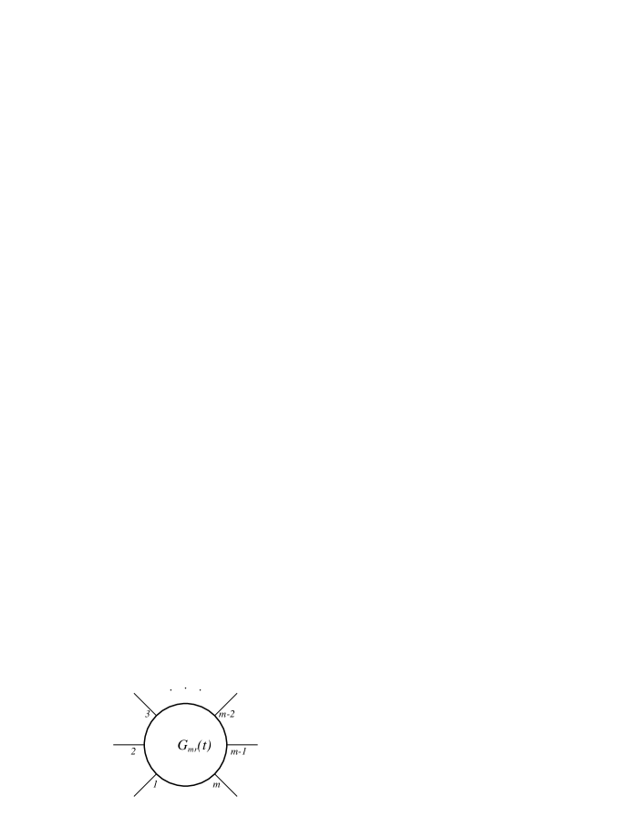
Figure 1: The vertex corresponding to $G_{mr}(t)$

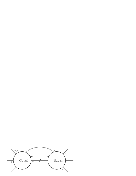
Figure 2: A graph contributing to the right hand side of the RGE

4 Fermionic sign cancellations

4.1 The determinant bound

Eq. $(\ref{Qrmtdef})$ already suggests that a determinant bound similar to the one used in Lemma 1 of [20] can be applied to the RGE. Before applying this bound, the derivative with respect to $t$ has to be performed, and some factors need to be arranged to avoid the factor ${\left|\Lambda\right|}$ that appeared in [20]. The reason it does not appear here is that only connected graphs contribute to the effective action (whereas the partition function itself was bounded in Lemma 1 of [20]). In the RGE, this is very easily seen without a reference to graphs.

Since the determinant is multilinear in the columns of the matrix, the derivative with respect to $t$ produces a sum of terms where every column gets differentiated. Expanding along each differentiated column gives

$$\frac{\partial}{\partial t}\det{\cal D}_{t}^{(i)}(\underline{V},\underline{W})=\sum\limits_{l=1}^{i}\sum\limits_{l^{\prime}=1}^{i}(-1)^{l+l^{\prime}}\dot{D}_{t}(V_{l},W_{l^{\prime}})\det{\cal D}_{t}^{(i-1)}(\underline{V}^{(l)},\underline{W}^{(l^{\prime})})$$ (60)

with $\underline{V}^{(l)}=(V_{1},\ldots,V_{l-1},V_{l+1},\ldots,V_{i})$ and a similar expression for $\underline{W}^{(l^{\prime})}$. The sign is cancelled by rearranging

$$G_{m_{1}r_{1}}(t\mid\underline{X}_{1},\underline{V}) = (-1)^{i-l}G_{m_{1}r_{1}}(t\mid\underline{X}_{1},\underline{V}^{(l)},V_{l})$$

$$G_{m_{2}r_{2}}(t\mid\underline{\tilde{W}},\underline{X}_{2}) = (-1)^{i-l^{\prime}}G_{m_{2}r_{2}}(t\mid W_{l^{\prime}},\underline{\tilde{W}}^{(l^{\prime})},\underline{X}_{2}).$$ (61)

Upon renaming of the integration variables, the summand becomes independent of $l$ and $l^{\prime}$, so the sum gives a factor $i^{2}$. Thus

$$Q_{mr}(t\mid\underline{X}) = \int d\kappa_{mr}\;i^{2}\int dV\;dW\;\dot{D}_{t}(V,W)\int d\underline{Y}\int d\underline{Z}$$

$$\det{\cal D}_{t}^{(i-1)}(\underline{Y},\underline{Z})G_{m_{1}r_{1}}(t\mid\underline{X}_{1},\underline{Y},V)G_{m_{2}r_{2}}(t\mid W,\underline{\tilde{Z}},\underline{X}_{2}).$$

Let $|\!|\!|\,\cdot\,|\!|\!|$ be the norm [14]

$$|\!|\!|F_{m}|\!|\!|=\max\limits_{p\in\{1,\ldots,m\}}\;\sup\limits_{X_{p}}\int\prod\limits_{q=1\atop q\neq p}^{m}dX_{q}\;{\left|F_{m}(X_{1},\ldots,X_{m})\right|}.$$ (63)

Lemma 1

Assume that

$$\sup\limits_{\underline{Y},\underline{Z}}{\left|\det{\cal D}_{t}^{(i-1)}(\underline{Y},\underline{Z})\right|}\leq A_{i-1}(t).$$ (64)

Then

$$|\!|\!|Q_{mr}(t)|\!|\!|\leq\int d\kappa_{mr}i^{2}A_{i-1}(t)\;|\!|\!|\dot{D}_{t}|\!|\!|\;|\!|\!|G_{m_{1}r_{1}}(t)|\!|\!|\;|\!|\!|G_{m_{2}r_{2}}(t)|\!|\!|.$$ (65)

Proof:     Let $p\in\{1,\ldots,m\}$. Without loss of generality, let $p\leq m_{1}-i$, so that $X_{p}$ is a component of $\underline{X}_{1}$ (the other case is similar by the symmetry of the sum for $Q_{mr}(t)$ in $m_{1}$ and $m_{2}$). By Eq. $(\ref{ati})$,

$$|\!|\!|Q_{mr}(t)|\!|\!|\leq\int d\kappa_{mr}i^{2}A_{i-1}(t)\;\sup\limits_{X_{p}}\int\prod\limits_{q=1\atop q\neq p}^{m_{1}-i}dX_{q}\int dV\;\phi(V,\underline{X}_{1})\;\chi(V)$$ (66)

with

$$\phi(V,\underline{X}_{1})=\int d\underline{Y}\;{\left|G_{m_{1}r_{1}}(t\mid\underline{X}_{1},\underline{Y},V)\right|}$$ (67)

and

$$\chi(V)=\int dW\;d\underline{Z}\;d\underline{X}_{2}\;{\left|\dot{D}_{t}(V,W)\right|}\;{\left|G_{m_{2}r_{2}}(t\mid W,\underline{\tilde{Z}},\underline{X}_{2})\right|}.$$ (68)

The bound

$$\chi(V)\leq\sup\limits_{V}\int dW{\left|\dot{D}_{t}(V,W)\right|}\sup\limits_{W}\int d\underline{Z}\;d\underline{X}_{2}\;{\left|G_{m_{2}r_{2}}(t\mid W,\underline{\tilde{Z}},\underline{X}_{2})\right|}$$ (69)

gives the result.  

From now on I assume that $\Lambda$ is a discrete torus and that ${\Lambda^{*}}$ is its dual. Let ${\cal N}$ be a set with $|{\cal N}|=n$ elements, let $\Gamma=\Lambda\times{\cal N}\times\{1,2\}$ and $\Gamma^{*}={\Lambda^{*}}\times{\cal N}\times\{1,2\}$. ${\cal N}$ can be thought of as the index set containing spin and colour indices. The last factor $\{1,2\}$ distinguishes between the usual $\psi$ and ${\bar{\psi}}$, as discussed in Section 2.

Lemma 2

Let $X=(x,\sigma,j)\in\Gamma$, and for every $k\in{\Lambda^{*}}$, let $M(k)$ be a symmetric matrix in ${\cal M}(n,{\mathbb{R}})$ with eigenvalues $m_{\rho}(k)$ satisfying $|m_{\rho}(k)|\leq 1$. Let $f_{t}:{\Lambda^{*}}\to{\mathbb{C}}$, and let

$$D_{t}(X,X^{\prime})=\delta_{j^{\prime},3-j}\int\limits_{{\Lambda^{*}}}dk\;{\rm e}^{ik(x-x^{\prime})}\;(-1)^{j}\;f_{t}((-1)^{j}k)M_{\sigma,\sigma^{\prime}}\left((-1)^{j}k\right)\;.$$ (70)

Then $D_{t}(X^{\prime},X)=-D_{t}(X,X^{\prime})$, and

$${\left|\det{\cal D}_{t}^{(i-1)}(\underline{Y},\underline{Z})\right|}\leq\left(\;\int\limits_{\Lambda^{*}}dk\;{\left|f_{t}(k)\right|}\right)^{i-1}.$$ (71)

Proof:     Since ${\Lambda^{*}}=-{\Lambda^{*}}$ and $(-1)^{j}=-(-1)^{j^{\prime}}$, a change of variables $k\to(-1)^{j}k$ implies

$$D_{t}(X,X^{\prime})=\delta_{j+j^{\prime},3}\;(-1)^{j}\;\int\limits_{{\Lambda^{*}}}dk\;f_{t}(k)\;M_{\sigma,\sigma^{\prime}}(k)\;{\rm e}^{ik((-1)^{j}x+(-1)^{j^{\prime}}x^{\prime})}.$$ (72)

The antisymmetry of $D_{t}$ now follows from the symmetry of $M$. Let $\Pi_{\rho}(k)$ be the spectral projection to the eigenspace of $m_{\rho}(k)$, so that $M(k)=\sum_{\rho}m_{\rho}(k)\Pi_{\rho}(k)$, and denote the scalar product on the spin space by $[\cdot,\cdot]$ so that $M(k)_{\sigma\sigma^{\prime}}=[e_{\sigma},M(k)\;e_{\sigma^{\prime}}]$, where the $e_{\sigma}$ are orthonormal. Then

$$D_{t}(X,X^{\prime}) = \int\limits_{{\Lambda^{*}}_{1}}dk\;\int\limits_{0}^{2\pi}\frac{d\varphi}{2\pi}\;\sum\limits_{\rho}\big{[}a_{t}(X)(k,\varphi,\rho),\;\Pi_{\rho}(k)\;b_{t}(X^{\prime})(k,\varphi,\rho)\big{]}$$ (73)

$$= \big{\langle}a_{t}(X)\;,\;b_{t}(X^{\prime})\big{\rangle}$$

with ${\Lambda^{*}}_{1}=\{k\in{\Lambda^{*}}:f_{t}(k)\neq 0\}$, and

$$a_{t}(X)(k,\varphi,\rho) = (-1)^{j}\;{\rm e}^{-ik(-1)^{j}x}\;{\rm e}^{-i\varphi(j-3)}|f_{t}(k)|^{1\over 2}e_{\sigma}$$

$$b_{t}(X^{\prime})(k,\varphi,\rho) = {\rm e}^{ik(-1)^{j^{\prime}}x^{\prime}}\;{\rm e}^{i\varphi j^{\prime}}\;f_{t}(k)m_{\rho}(k)\;|f_{t}(k)|^{-{1\over 2}}e_{\sigma^{\prime}}.$$ (74)

Gram’s bound [36],

$${\left|\det{\cal D}_{t}^{(i-1)}(\underline{Y},\underline{Z})\right|}\leq\prod\limits_{k=1}^{i-1}\Big{(}\langle a_{t}(Y_{k}),a_{t}(Y_{k})\rangle\;\langle b_{t}(Z_{k}),b_{t}(Z_{k})\rangle\Big{)}^{1\over 2},$$ (75)

and

$$\sum\limits_{\rho}|m_{\rho}(k)|^{2}\langle e_{\sigma},\Pi_{\rho}(k)e_{\sigma}\rangle\leq\sum\limits_{\rho}\langle e_{\sigma},\Pi_{\rho}(k)e_{\sigma}\rangle\leq 1$$ (76)

imply Eq. $(\ref{grambound})$.  

Corollary 1

If $f_{t}(k)={\tilde{D}_{t}}(k)$ and $M_{\sigma\sigma^{\prime}}(k)=\delta_{\sigma\sigma^{\prime}}$ (as in the above many-fermion systems) then

$$|\det{\cal D}_{t}^{(i-1)}(\underline{Y},\underline{Z})|\leq\left(\int_{\Lambda^{*}}dk\;{\left|{\tilde{D}_{t}}(k)\right|}\right)^{i-1}.$$ (77)

4.2 Power counting for point singularities

In this section, I show some basic power counting bounds for the Green functions obtained from the truncation that all marginal or relevant couplings are left out.

Theorem 1

Assume that $D_{t}$ is of the form Eq. $(\ref{Dform})$, that

$$\int\limits_{\Lambda^{*}}dk\;{\left|{\tilde{D}_{t}}(k)\right|}\leq\Delta_{1}{\rm e}^{-t},$$ (78)

and that

$$|\!|\!|\dot{D}_{t}|\!|\!|\leq\Delta_{2}{\rm e}^{t}.$$ (79)

Let $\int d\tilde{\kappa}_{mr}$ denote the measure obtained by restricting the sum in $\int d\kappa_{mr}$ to $m_{1}\geq 4$ and $m_{2}\geq 4$ and replacing $G_{4,r_{k}}$ by $v\delta_{r_{k},1}$ whenever it appears in the sum on the right hand side of Eq. $(\ref{Qrmtdef})$. Then the solution $\tilde{G}_{mr}(t)$ of Eq. $(\ref{comRGE})$ with initial condition $G_{mr}(0)=G_{mr}^{(0)}$ satisfies

$$|\!|\!|\tilde{G}_{mr}(t)|\!|\!|\leq\cases{\gamma_{mr}{\rm e}^{t({m\over 2}-2)}&if $m\geq 6$\cr\gamma_{4r}(1+t)&if $m=4$\cr\gamma_{2r}&if $m=2$}$$ (80)

with $\gamma_{mr}$ defined recursively as

$$\gamma_{mr}=|\!|\!|G_{mr}^{(0)}|\!|\!|+3\Delta_{2}\frac{1}{m}\int d\tilde{\kappa}_{mr}i^{2}\Delta_{1}^{i-1}\gamma_{m_{1}r_{1}}\gamma_{m_{2}r_{2}}.$$ (81)

Proof:     Induction in $r$, with Eq. $(\ref{nppoco})$ and Eq. $(\ref{Recu})$ as the inductive hypothesis. The case $r=1$ is trivial. Let $r\geq 2$, and the statement hold for all $r^{\prime}<r$. By Lemma 2, Eq. $(\ref{ati})$ holds with $A_{i}(t)=\Delta_{1}^{i-1}{\rm e}^{-t(i-1)}$. Thus

$$|\!|\!|Q_{mr}(t)|\!|\!|\leq\Delta_{2}\int d\tilde{\kappa}_{mr}i^{2}\Delta_{1}^{i-1}{\rm e}^{-t(i-2)}|\!|\!|\tilde{G}_{m_{1}r_{1}}(t)|\!|\!|\;|\!|\!|\tilde{G}_{m_{2}r_{2}}(t)|\!|\!|.$$ (82)

By the inductive hypothesis and $m_{1}+m_{2}-2i=m$, $|\!|\!|\,\cdot\,|\!|\!|$ of the right hand side of Eq. $(\ref{icomRGE})$ is bounded by

$$|\!|\!|G_{mr}(0)|\!|\!|+\int d\tilde{\kappa}_{mr}i^{2}\Delta_{1}^{i-1}\Delta_{2}\gamma_{m_{1}r_{1}}\gamma_{m_{2}r_{2}}\;\frac{1}{2}\int\limits_{0}^{t}ds\;{\rm e}^{s({m\over 2}-2)}$$ (83)

To complete the induction step, this has to be bounded by the right hand side of Eq. $(\ref{nppoco})$. If $m\geq 6$, $\frac{m}{2}-2\geq\frac{m}{6}\geq 1$, so

$$\frac{1}{2}\int\limits_{0}^{t}ds\;{\rm e}^{s({m\over 2}-2)}\leq\frac{1}{m-4}{\rm e}^{t({m\over 2}-2)}\leq\frac{3}{m}{\rm e}^{t({m\over 2}-2)}.$$ (84)

If $m=4$, $\frac{1}{2}\int_{0}^{t}ds\leq\frac{2}{m}(1+t)$. If $m=2$, $\frac{m}{2}-2=-1$, so $\frac{1}{2}\int_{0}^{t}ds\;{\rm e}^{s({m\over 2}-2)}\leq{\textstyle\frac{1}{2}}={\textstyle\frac{1}{m}}$. This implies Eq. $(\ref{nppoco})$, with $\gamma_{mr}$ given by Eq. $(\ref{Recu})$.  

Remark 1

In graphical language, the truncation removes all two-legged and all nontrivial fourlegged insertions (‘nontrivial’ means that the four-legged vertices are still there).

Remark 2

The solution to Eq. $(\ref{Recu})$ is bounded by the solution to the untruncated recursion $\gamma_{m1}=v\delta_{m4}$, and for $r\geq 2$,

$$\gamma_{mr}=\gamma_{mr}^{(0)}+A\frac{1}{m}\int d\kappa_{mr}i^{2}B^{i-1}\gamma_{m_{1}r_{1}}\gamma_{m_{2}r_{2}}$$ (85)

with $A=3\Delta_{2}$ and $B=\Delta_{1}$. The constants $A$ and $B$ can be scaled out of the recursion. If the initial interaction is a four-fermion interaction, $g_{m,r}=m\gamma_{mr}A^{-1}B^{1-{m\over 2}}$ satisfies the recursion $g_{m,1}=w\delta_{m4}$, with $w=4AB$, and for $r\geq 2$,

$$g_{m,r}=\sum\limits_{s=1}^{r-1}\sum\limits_{k\geq 0}\sum\limits_{\mu=2\atop\mu\;\rm even}^{2(s+1)}{\mu-1\choose k}{m+2k+1-\mu\choose k}g_{\mu,s}\;g_{m+2k+2-\mu,r-s}.$$ (86)

I do not provide bounds for the solution $g_{m,r}$ here; if $g_{m,r}\leq\hbox{ \rm const }^{r}$, then the above bounds imply that $\sum_{r}\lambda^{r}\tilde{G}_{mr}(t)$ is analytic in $\lambda$. This behaviour is suggested by the absence of the factor $i!$ that would appear for bosons in the recursion; see [13].

The propagators $C_{t}$ and $D_{t}$ for the renormalization group equation are defined using a partition of unity $\chi_{1}+\chi_{2}=1$, $\chi_{i}\in C^{\infty}({\mathbb{R}}^{+}_{0},[0,1])$ with

$$\chi_{1}(x)=\cases{1&if $x\leq\frac{1}{4}$\cr 0&if $x\geq 1$}$$ (87)

$\chi_{1}^{\prime}(x)<0$ for all $x\in(\frac{1}{4},1)$, and ${\left\|\chi_{1}^{\prime}\right\|}_{\infty}\leq 2$.

Proposition 3

Let $\Lambda$ be $d$-dimensional, and ${\cal B}$ be the infinite-volume limit of ${\Lambda^{*}}$. For instance, for $\Lambda=\varepsilon{\mathbb{Z}}^{d}/L{\mathbb{Z}}^{d}$, with ${\textstyle\frac{L}{2\varepsilon}}\in 2{\mathbb{N}}$, ${\cal B}={\mathbb{R}}^{d}/{\textstyle\frac{2\pi}{\varepsilon}}{\mathbb{Z}}^{d}$. Let $D_{t}$ be given by Eq. $(\ref{Dform})$ with ${\left\|M(k)\right\|}\leq 1$, $f_{t}(0)=0$, and for $k\neq 0$

$$f_{t}(k)=\tilde{f}(k)\chi_{1}({\rm e}^{2t}\tilde{f}(k)^{2}),$$ (88)

with $\tilde{f}\in C^{d+1}({\cal B}\setminus\{0\},{\mathbb{C}})$, satisfying for all $|\alpha|\leq d+1$ and all $|k|\leq 1$, $|D^{\alpha}\tilde{f}(k)|\leq F_{d}|k|^{1-d-|\alpha|}$. Then Eq. $(\ref{einnorm})$ and Eq. $(\ref{sumnorm})$ hold.

Proof:     Eq. $(\ref{einnorm})$ holds because $\int_{{\Lambda^{*}}\setminus\{0\}}|k|^{1-d}\chi_{1}(k^{2}{\rm e}^{2t})dk$ is a Riemann sum approximation to the convergent integral $\int_{\cal B}|k|^{1-d}\chi_{1}(k^{2}{\rm e}^{2t}){\textstyle\frac{d^{d}k}{(2\pi)^{d}}}$. The infinite-volume analogue of Eq. $(\ref{sumnorm})$ is usually proven by integration by parts, using repeatedly

$$(x_{\nu}-x_{\nu}^{\prime})D_{t}(x-x^{\prime})=-\int\limits_{\cal B}\frac{d^{d}k}{(2\pi)^{d}}{\rm e}^{{\rm i}(x-x^{\prime})k}\frac{\partial}{\partial k_{\nu}}\hat{D}_{t}(k),$$ (89)

which implies that $|D_{t}(X,X^{\prime})|$ falls off at least as $(1+{\rm e}^{-t}|x-x^{\prime}|)^{-d-1}$ for large $|x-x^{\prime}|$. On the torus at finite $L$, one iterates instead the summation by parts formula

$$D(x-x^{\prime})(1-{\rm e}^{{\rm i}a(x-x^{\prime})})=\int\limits_{\Lambda^{*}}dk\;{\rm e}^{{\rm i}k(x-x^{\prime})}\left(\hat{D}(k)-\hat{D}(k-a)\right)$$ (90)

which holds for all $a\in{\Lambda^{*}}$, decomposes $\Lambda$ into $2^{d}$ parts and chooses $a$ appropriately to get an analogue of Eq. $(\ref{original})$. This works uniformly in $L$ because $M(0)=0$. A similar argument is given in more detail in the proof of Lemma 5.  

Remark 3

Let $d\geq 2$, $\Lambda=\varepsilon{\mathbb{Z}}^{d}/L{\mathbb{Z}}^{d}$ and

$$L_{\varepsilon}(k)=\frac{2}{\varepsilon^{2}}\sum\limits_{\nu=1}^{d}(1-\cos(\varepsilon k_{\nu})).$$ (91)

The choices $\tilde{f}(k)=L_{\varepsilon}(k)^{{1-d\over 2}}$, $M=1$ (the toy model of [20]), and

$$\tilde{f}(k)=\left(\sum\limits_{\nu=1}^{d}\left(\frac{1}{\varepsilon}\sin(k_{\nu}\varepsilon)\right)^{2}+(\varepsilon L_{\varepsilon}(k))^{2}\right)^{-1/2}$$ (92)

and

$$M(k)=\tilde{f}(k)\left(\sum\limits_{\nu=1}^{d}{\rm i}\gamma_{\nu}\frac{1}{\varepsilon}\sin(k_{\nu}\varepsilon)+\varepsilon L_{\varepsilon}(k)\right)$$ (93)

(Wilson fermions) satisfy the hypotheses of Proposition 3. For all $t>0$, the infinite-volume limit $L\to\infty$ and the continuum limit $\varepsilon\to 0$ of the Green functions $\tilde{G}_{mr}(t)$ exist and satisfy Eq. $(\ref{nppoco})$. In the first case, $\tilde{f}(k)\to|k|^{1-d}$, in the second case, $M(k)\tilde{f}(k)\to{\textstyle\frac{/\mkern-10.0mup}{p^{2}}}$ as $\varepsilon\to 0$. The Euclidean Dirac matrices satisfy the Clifford algebra $\gamma_{\mu}\gamma_{\nu}+\gamma_{\nu}\gamma_{\mu}=\delta_{\mu\nu}$, and can be chosen hermitian, $\gamma_{\mu}^{*}=\gamma_{\mu}$. It is possible to adapt the matrix structure of Lemma 2 to satisfy the antisymmetry condition on $D_{t}$ also for this case.

Remark 4

In ultraviolet renormalizable theories, the signs in the exponents of Eq. $(\ref{einnorm})$ and Eq. $(\ref{sumnorm})$ are reversed. A power counting theorem similar to the infrared power counting Theorem 1 can be proven provided that in the initial interaction, at most quartic interactions appear. The statement is then that for $m\geq 6$, the Green function is bounded by $\hbox{ \rm const }{\rm e}^{-t({m\over 2}-2)}$.

5 The thermodynamic limit of the many-fermion system

In this section, I apply the RGE to the many-fermion systems defined in Section 2. For $d=1$, the singularity is pointlike, so the power counting bound Theorem 1 applies. For $d\geq 2$, the analogue of Theorem 1 gives only weaker bounds, which, e.g., in $d=2$ would mean that the four-point function is still relevant and the six-point function is marginal. This is not the actual behaviour; showing better bounds in $d\geq 2$ requires a refinement using the sector technique of [20] and is deferred to another paper. I also show a simple bound for the full Green functions that takes into account the sign cancellations. If the coefficients $\gamma_{mr}$ given by Eq. $(\ref{untrecu})$ are exponentially bounded, this bound implies that the unrenormalized expansion converges in a region $|\lambda|\beta^{d}<\hbox{ \rm const }$. I also give a simple proof that the thermodynamic limit exists in perturbation theory.

One can also show bounds on the expansion coefficients for finite $n_{\tau}$ and $L$. Since this is mainly a tedious repetition of the infinite-volume proofs with integrals replaced by Riemann sums (it also requires that $\mu$ is chosen such that the Fermi surface contains no points of the finite-$L$ momentum space lattice), I will content myself with indicating where this is necessary.

For convenience, I call the limit $n_{\tau}\to\infty$ and $L\to\infty$ the thermodynamic limit, although the first limit would more aptly be called the time-continuum limit. The limit $n_{\tau}\to\infty$ has to be taken first, because I want to apply Eq. $(\ref{Trotto})$ for operators on a finite-dimensional space only. However, it will turn out that for $T>0$, the order of the two limits does not matter. Since I want to take the limit $n_{\tau}\to\infty$, I can assume that $n_{\tau}\geq 2\beta(\epsilon_{0}+E_{\rm max})$. Thus Lemma 9 applies, with $E_{0}=\epsilon_{t}$, for all $t\geq 0$.

5.1 The component RGE in Fourier space

Let $\Lambda={\mathbb{T}}\times{\mathbb{L}}$ and ${\Lambda^{*}}={\mathbb{M}}_{n_{\tau}}\times{\mathbb{L}}^{*}$, as given in Sections 2.1 and 2.2. Let $\Gamma=\Lambda\times\{-1,1\}\times\{1,2\}$ and ${\Gamma^{*}}={\Lambda^{*}}\times\{-1,1\}\times\{1,2\}$. The Fourier transforms of the $G_{mr}(t)$ are, with $(\underline{P}=(P_{1},\ldots,P_{m})$,

$$\hat{G}_{mr}(t\mid\underline{P})=\int\limits_{\Lambda^{m}}\prod\limits_{k=1}^{m}dx_{k}\;{\rm e}^{-{\rm i}(p_{1}x_{1}+\ldots+p_{m}x_{m})}G_{mr}(t\mid\underline{X}).$$ (94)

For $K=(k,\sigma,j)\in{\Gamma^{*}}$ let $\sim K=(-k,\sigma,3-j)$, and let $\delta_{{\Gamma^{*}}}(K,K^{\prime})=\delta_{{\Lambda^{*}}}(k,k^{\prime})\delta_{\sigma\sigma^{\prime}}\delta_{jj^{\prime}}$. Assume that the Fourier transform of the propagator $D_{t}$ is of the form

$$\hat{D}_{t}(K,K^{\prime})=\delta_{{\Gamma^{*}}}(K,\sim K^{\prime})\;\bar{D}_{t}(K^{\prime})$$ (95)

where

$$\bar{D}_{t}(K)=(-1)^{j}{\tilde{D}_{t}}((-1)^{j}k).$$ (96)

This combination of signs implies that $D_{t}(X,Y)=-D_{t}(Y,X)$. The propagator ${\tilde{D}_{t}}$ for the many-fermion system is given in Eq. $(\ref{e112})$. The Fourier transform of $Q_{mr}(t)$ is

$$\hat{Q}_{mr}(t\mid\underline{P}) = \int d\kappa_{mr}\;i!i\int dK_{1}\ldots dK_{i}\;(-\dot{\bar{D}_{t}}(K_{1}))\;\prod\limits_{j=2}^{i}\bar{D}_{t}(K_{j})$$ (97)

$$\hat{G}_{m_{1}r_{1}}(t\mid\underline{P}^{(1)},\underline{K})\;\hat{G}_{m_{2}r_{2}}(t\mid\sim\underline{K},\underline{P}^{(2)})$$

with $\underline{P}^{(1)}=(P_{1},\ldots,P_{m_{1}-i})$, $\underline{P}^{(2)}=(P_{m_{1}-i+1},\ldots,P_{m_{1}+m_{2}})$, $\underline{K}=(K_{1},\ldots,K_{i})$, and $\sim\underline{K}=(\sim K_{i},\ldots,\sim K_{1})$. Here the arguments of $G_{m_{2}r_{2}}(t)$ have been permuted and relabelled such that the determinant is transformed into a sum with the same sign for all terms (see Appendix C); this gives the extra factor $i!$.

By translation invariance in space ${\bf x}$ and time $\tau$,

$$\hat{G}_{mr}(t\mid P_{1},\ldots,P_{m})=\delta_{{\Lambda^{*}}}(p_{1}+\ldots+p_{m},0)I_{mr}(t\mid P_{1},\ldots,P_{m})$$ (98)

with a totally antisymmetric function $I_{mr}(t\mid P_{1},\ldots,P_{m})$ of $(P_{1},\ldots,P_{m})\in{\Gamma^{*}}^{m}$ that satisfies

$$\sum\limits_{\mu=1}^{m}\nabla_{p_{\mu}}I_{mr}(t\mid P_{1},\ldots,P_{m})=0.$$ (99)

A priori, Eq. $(\ref{Idelta})$ implies only the existence of a function $\hat{I}_{mr}(t\mid P_{1},\ldots,P_{m})$, defined only for those $P_{1},\ldots,P_{m}$ for which $p_{1}+\ldots+p_{m}=0$. However, since $H=\{{p_{1},\ldots,p_{m}}:\;p_{1}+\ldots+p_{m}=0\}$ is a linear subspace of $({\Lambda^{*}})^{m}$, one can simply extend $\tilde{I}$ to a function on all space by defining $I=\hat{I}\circ\Pi_{H}$ with $\Pi_{H}$ the projection to the subspace $H$. Since $\Pi_{H}$ is symmetric in all its arguments, $I$ is totally antisymmetric, and Eq. $(\ref{senkre})$ holds because $(1,\ldots,1)\perp H$ (in Eq. $(\ref{senkre})$, $\nabla_{p_{\mu}}$ is a difference operator which becomes the gradient in the limit where the momenta become continuous).

The product of the two $\delta_{\Lambda^{*}}$ in Eq. $(\ref{Qfour1})$ can be combined to cancel the $\delta_{\Lambda^{*}}$ in the relation between $\hat{G}$ and $I$, and to remove the integration over $k_{1}$. Thus the RGE in Fourier space is ${\textstyle\frac{\partial}{\partial t}}I_{mr}(t\mid\underline{P})=\frac{1}{2}{\mathbb{A}}_{m}Q_{mr}(t\mid\underline{P})$, with

$$Q_{mr}(t\mid\underline{P}) = \int d\kappa_{mr}\;i!i\;\int dK_{2}\ldots dK_{i}\sum\limits_{\sigma_{1},j_{1}}(-\dot{\bar{D}_{t}}(K_{1}))\;$$ (100)

$$\prod\limits_{s=2}^{i}\bar{D}_{t}(K_{s})\;I_{m_{1}r_{1}}(t\mid\underline{P}^{(1)},\underline{K})\;I_{m_{2}r_{2}}(t\mid\sim\underline{K},\underline{P}^{(2)})$$

where $K_{1}=(k_{1},\sigma_{1},j_{1})$ and $k_{1}$ is fixed as $k_{1}=-(k_{2}+\ldots+k_{i})+p_{1}+\ldots+p_{m_{1}-i+1}$. I use the same symbol for the $Q$ in position and in momentum space since it will be always clear from the context which one is meant.

Remark 5

The equivalent integral equation is

$$I_{mr}(t\mid\underline{P})=I_{mr}(0\mid\underline{P})+\frac{1}{2}{\mathbb{A}}_{m}\;\int\limits_{0}^{t}ds\;Q_{mr}(s\mid\underline{P}).$$ (101)

The sum $\int d\kappa_{mr}$ contains the sum over $r_{1}\geq 1$ and $r_{2}\geq 1$, with the restriction $r_{1}+r_{2}=r$. Thus only $r_{1}<r$ and $r_{2}<r$ occur in this sum. Therefore Eq. $(\ref{equinteFou})$, together with an initial condition $I_{mr}(0\mid\underline{P})$, uniquely determines the family of functions $I_{mr}(t\mid\underline{P})$. Iteration of Eq. $(\ref{equinteFou})$ generates the usual perturbation expansion.

5.2 Bounds on the finite-volume propagator

The propagator $\hat{c}$ for the many-fermion system is given in Eq. $(\ref{mfprop1})$. If ${\bf k}$ is such that $E({\bf k})=0$, then $\hat{c}$ becomes of order $\beta$ for small $|\omega|$. In the temperature zero limit, $\beta\to\infty$, this becomes a singularity. This is the reason why renormalization is necessary. The renormalization group flow is parametrized by $t\geq 0$, where

$$\epsilon_{t}=\epsilon_{0}{\rm e}^{-t}$$ (102)

is a decreasing energy scale. The fixed energy scale $\epsilon_{0}$ was specified in Section 2.3. The limit of interest is $t\to\infty$.

The uncutoff propagator for the many-fermion system is given in Eq. $(\ref{mfprop1})$. Thus, for $k=(\omega,{\bf k})\in{\Lambda^{*}}$ let

$${\tilde{D}_{t}}(k)=\frac{1}{{\rm i}\widehat{\omega}-E({\bf k})}\;\chi_{1}\left({\epsilon_{t}}^{-2}{\left|{\rm i}\widehat{\omega}-E({\bf k})\right|}^{2}\right)$$ (103)

where $\widehat{\omega}$ is defined in Eq. $(\ref{Hatomdef})$, $\chi_{1}$ is given in Eq. $(\ref{zerleg})$, and define $\tilde{C}_{t}(k)$ similarly, with $\chi_{1}$ replaced by $\chi_{2}=1-\chi_{1}$. Then $\tilde{C}_{t}(k)+{\tilde{D}_{t}}(k)=({\rm i}\widehat{\omega}-E({\bf k}))^{-1}$ is independent of $t$. The functions $\tilde{C}_{t}$ and ${\tilde{D}_{t}}$ define operators $\hat{D}_{t}(K,K^{\prime})$ and $\hat{C}_{t}(K,K^{\prime})$ on the functions on ${\Gamma^{*}}$ by Eq. $(\ref{e94})$ and Eq. $(\ref{e93})$. Denote $\dot{\tilde{D}_{t}}=\frac{\partial}{\partial t}{\tilde{D}_{t}}$, and let $\;{\mathchoice{\rm 1\mskip-4.0mul}{\rm 1\mskip-4.0mul}{\rm 1\mskip-4.5mul}{\rm 1\mskip-5.0mul}}\left(A\right)\;=1$ if the event $A$ is true and $0$ otherwise.

Proposition 4

${\tilde{D}_{t}}$ is a $C^{\infty}$ function of $t$ that vanishes identically if $t>\log\frac{\beta\epsilon_{0}}{2}$. If $t\leq log\frac{\beta\epsilon_{0}}{2}$, then

$$\mbox{ \rm supp }{\tilde{D}_{t}} \subset \{k\in{\Lambda^{*}}:{\left|{\rm i}\widehat{\omega}-E({\bf k})\right|}\leq\epsilon_{t}\}$$

$$\mbox{ \rm supp }\dot{\tilde{D}_{t}} \subset \{k\in{\Lambda^{*}}:\frac{1}{2}\epsilon_{t}\leq{\left|{\rm i}\widehat{\omega}-E({\bf k})\right|}\leq\epsilon_{t}\}.$$ (104)

Moreover

$${\left|\dot{\tilde{D}_{t}}(k)\right|}\leq 4\epsilon_{t}^{-1}\;{\mathchoice{\rm 1\mskip-4.0mul}{\rm 1\mskip-4.0mul}{\rm 1\mskip-4.5mul}{\rm 1\mskip-5.0mul}}\left({\left|{\rm i}\widehat{\omega}-E({\bf k})\right|}\leq\epsilon_{t}\right)\;\\ \leq 2\beta\;{\mathchoice{\rm 1\mskip-4.0mul}{\rm 1\mskip-4.0mul}{\rm 1\mskip-4.5mul}{\rm 1\mskip-5.0mul}}\left({\left|{\rm i}\widehat{\omega}-E({\bf k})\right|}\leq\epsilon_{t}\right)\;,$$

${\left|{\tilde{D}_{t}}(k)\right|}\leq\frac{\beta}{2}\;{\mathchoice{\rm 1\mskip-4.0mul}{\rm 1\mskip-4.0mul}{\rm 1\mskip-4.5mul}{\rm 1\mskip-5.0mul}}\left({\left|{\rm i}\widehat{\omega}-E({\bf k})\right|}\leq\epsilon_{t}\right)\;$,

$$\int\limits_{\Lambda^{*}}dk\;{\left|\dot{\tilde{D}_{t}}(k)\right|}\leq 4{{\cal V}_{1}}\quad\mbox{ and }\quad\int\limits_{\Lambda^{*}}dk\;{\left|{\tilde{D}_{t}}(k)\right|}\leq{{\cal V}_{1}}\log{\textstyle\frac{\beta\epsilon_{0}}{2}},$$ (105)

where ${{\cal V}_{1}}$ is the constant in Eq. $(\ref{Vobou})$.

Proof:     $\chi_{1}(x)=0$ if $x\geq 1$, so ${\tilde{D}_{t}}(k)\neq 0$ implies ${\left|{\rm i}\widehat{\omega}-E({\bf k})\right|}\leq\epsilon_{t}\leq 1$. By Lemma 9, this implies $|\omega|\leq{\textstyle\frac{\pi}{2}}\epsilon_{t}$. Since $|\omega|\geq{\textstyle\frac{\pi}{\beta}}$, ${\tilde{D}_{t}}\neq 0$ only for $t\leq\log{\textstyle\frac{\beta\epsilon_{0}}{2}}$. Since $|{\rm i}\widehat{\omega}-E({\bf k})|\geq|\mbox{Re }\widehat{\omega}|\geq{\textstyle\frac{2}{\beta}}$, the stated properties of ${\tilde{D}_{t}}$ follow. The $t$-derivative gives $|{\textstyle\frac{\partial}{\partial t}}{\tilde{D}_{t}}(k)|=2\epsilon_{t}^{-2}|{\rm i}\widehat{\omega}-E({\bf k})|\;|\chi_{1}^{\prime}(\epsilon_{t}^{-2}|{\rm i}\widehat{\omega}-E({\bf k})|^{2})|$. Since $\chi_{1}^{\prime}(x)=0$ for $x\not\in(\frac{1}{4},1)$, $\dot{\tilde{D}_{t}}(k)\neq 0$ implies ${\textstyle\frac{1}{2}}\epsilon_{t}\leq{\left|{\rm i}\widehat{\omega}-E({\bf k})\right|}\leq\epsilon_{t}$ which implies Eq. $(\ref{cwtdbe})$ and Eq. $(\ref{cwtsupp})$. Eq. $(\ref{cwtint})$ follows from these inequalities by Lemma 9, by Eq. $(\ref{Vobou})$, and by ${\tilde{D}_{t}}=\int_{t}^{\log(\beta\epsilon_{0}/2)}ds\;\dot{\tilde{D}_{s}}$.  

Remark 6

The bounds Eq. $(\ref{cwtint})$ are crude because the restriction $|E({\bf k})|\leq\epsilon_{t}$ was replaced by $|E({\bf k})|\leq 2$ when Eq. $(\ref{Vobou})$ was applied. To get a better bound, one has to require that no points of the finite–volume lattice in momentum space is on the Fermi surface ${\cal S}$. Because only then $\int_{\mathbb{L}}dk\;{\mathchoice{\rm 1\mskip-4.0mul}{\rm 1\mskip-4.0mul}{\rm 1\mskip-4.5mul}{\rm 1\mskip-5.0mul}}\left(|E({\bf k})|\leq\epsilon_{t}\right)\;\leq\hbox{ \rm const }\epsilon_{t}$ holds uniformly in $L$.

5.3 Existence of the thermodynamic limit in perturbation theory

The proof of existence of the thermodynamic limit will proceed inductively in $r$, because of the recursive structure of the RGE mentioned in Remark 5. It will be an application of the dominated convergence theorem to Eq. $(\ref{equinteFou})$. To this end, it is necessary to make the integration region independent of $n_{\tau}$ and $L$. Although ${I_{mr}}(t)$, given by Eq. $(\ref{equinteFou})$, appears evaluated at $\underline{P}=(P_{1},\ldots,P_{m})\in\Gamma^{m}$ on the RHS of Eq. $(\ref{equinteFou})$ only, the integral defines the $t$-derivative of a function defined on ${\Gamma^{*}_{\infty}}^{m}$, where ${\Gamma^{*}_{\infty}}={\mathbb{M}}(\beta)\times{\cal B}\times\{1,-1\}\times\{1,2\}$ with ${\cal B}={\mathbb{G}}^{*}$ the first Brillouin zone of the infinite lattice, and

$${\mathbb{M}}(\beta)=\{\omega_{n}=\frac{\pi}{\beta}(2n+1):\;n\in{\mathbb{Z}}\}$$ (106)

the set of Matsubara frequencies in the limit $n_{\tau}\to\infty$. For a bounded function $F_{m}:{\Gamma^{*}_{\infty}}^{m}\to{\mathbb{C}}$, let

$${\left|F_{m}\right|}_{0}=\sup\limits_{\underline{P}\in{\Gamma^{*}_{\infty}}^{m}}{\left|F_{m}(\underline{P})\right|}$$ (107)

Up to now, the dependence of ${I_{mr}}(t)$ on $(n_{\tau},L)$ was not denoted explicitly. I now put it in a superscript and write $I_{mr}^{(n_{\tau},L)}$. Let $\lim\limits_{(n_{\tau},L)\to\infty}=\lim_{L\to\infty}\lim_{n_{\tau}\to\infty}$.

Lemma 3

Let $(I_{mr}^{(n_{\tau},L)}(0))_{m,r,n_{\tau},L}$ be a family of bounded functions such that $I_{mr}^{(n_{\tau},L)}(0)=0$ if $m>2r+2$, $\lim_{(n_{\tau},L)\to\infty}I_{mr}^{(n_{\tau},L)}(0)={I_{mr}}(0)$ exists and is a bounded function on ${\Gamma^{*}_{\infty}}^{m}$, and ${\left|I_{mr}^{(n_{\tau},L)}(0)\right|}\leq K_{mr}^{(0)}$. Let $(I_{mr}^{(n_{\tau},L)}(t))_{m,r,n_{\tau},L}$ be the solution to Eq. $(\ref{equinteFou})$. Then, for all $m$ and $r$, $I_{mr}^{(n_{\tau},L)}(t)=0$ if $m>2r+2$, and

$$\frac{\partial}{\partial t}I_{mr}^{(n_{\tau},L)}(t)=0\quad\mbox{ for all }t>\log\frac{\beta}{2},$$ (108)

there are bounded functions ${I_{mr}}(t):{\Gamma^{*}_{\infty}}^{m}\to{\mathbb{C}}$ such that

$$\lim\limits_{(n_{\tau},L)\to\infty}I_{mr}^{(n_{\tau},L)}(t)={I_{mr}}(t).$$ (109)

Let $P_{mr}$ be the polynomials defined recursively as

$$P_{mr}(x)=6^{1-r}|{I_{mr}}(0)|+\epsilon_{0}^{-1}\int d\kappa_{mr}i\;i!\;x^{i-1}P_{m_{1}r_{1}}(x)P_{m_{2}r_{2}}(x)$$ (110)

(in particular, the coefficients of $P_{mr}$ are independent of $\beta$), then for all $n_{\tau},L,\beta,t$

$${\left|I_{mr}^{(n_{\tau},L)}(t)\right|}_{0}\leq(\epsilon_{0}\beta)^{r-1}P_{mr}\left(4{{\cal V}_{1}}\log{\textstyle\frac{\beta\epsilon_{0}}{2}}\right).$$ (111)

Proof:     Induction in $r$, with the statement of the Lemma as the inductive hypothesis. Let $r=1$. Since $r_{1}\geq 1$ and $r_{2}\geq 1$, the right hand side of the equation is zero, so $I_{m1}^{(n_{\tau},L)}(t,\underline{P})=I_{m1}^{(n_{\tau},L)}(0,\underline{P})$ for all $t$. Thus the statement follows from the hypotheses on $I_{mr}^{(n_{\tau},L)}(0)$.

Let $r\geq 2$, and the statement hold for all $r^{\prime}<r$. Let $m>2r+2$. Then $I_{mr}^{(n_{\tau},L)}(0)=0$. The five-tuple $(m_{1},r_{1},m_{2},r_{2},i)$ contributes to the right hand side only if $r_{1}+r_{2}=r$, $m_{1}+m_{2}=m+2i$, $i\geq 1$, and by the inductive hypothesis, only if $m_{1}\leq 2r_{1}+2$ and $m_{2}\leq 2r_{2}+2$. Thus $I_{mr}^{(n_{\tau},L)}(t)$ can be nonzero only if $m=m_{1}+m_{2}-2i\leq m_{1}+m_{2}-2\leq 2r_{1}+2+2r_{2}+2-2=2r+2$. The integral appearing on the right hand side of Eq. $(\ref{equinteFou})$ is a Riemann sum approximation to an integral over the $(t,n_{\tau},L)$-independent region $s\in[0,\infty)$, $k_{j}\in{\mathbb{M}}(\beta)\times{\cal B}$. By the inductive hypothesis, the factors $I_{m_{k}r_{k}}^{(n_{\tau},L)}$ have a limit Eq. $(\ref{ih3})$ satisfying Eq. $(\ref{ih4})$. Since for all $t$, $\bar{D}_{t}$ is a bounded $C^{2}$ function, the same holds for the propagators (boundedness holds because $\beta<\infty$). Thus the integrand converges pointwise, and it suffices to show that it is bounded by an integrable function to get Eq. $(\ref{ih3})$ and Eq. $(\ref{ih4})$ by an application of the dominated convergence theorem. Let $\alpha=4{{\cal V}_{1}}\log{\textstyle\frac{\beta\epsilon_{0}}{2}}$, and let $g$ be the function on $[0,\infty)\times({\mathbb{M}}(\beta)\times{\cal B})^{i-1}$ given by

$$g(s,\underline{k}) = \frac{2}{\epsilon_{0}{\rm e}^{-s}}\;{\mathchoice{\rm 1\mskip-4.0mul}{\rm 1\mskip-4.0mul}{\rm 1\mskip-4.5mul}{\rm 1\mskip-5.0mul}}\left(s\leq\log{\textstyle\frac{\beta\epsilon_{0}}{2}}\right)\;\int d\kappa_{mr}\;i\;i!P_{m_{1}r_{1}}(\alpha)\beta^{r_{1}-1}P_{m_{2}r_{2}}(\alpha)\beta^{r_{2}-1}$$ (112)

$$\prod\limits_{j=2}^{i}\int\limits_{0}^{s}ds_{j}\;{\mathchoice{\rm 1\mskip-4.0mul}{\rm 1\mskip-4.0mul}{\rm 1\mskip-4.5mul}{\rm 1\mskip-5.0mul}}\left(|\omega_{j}|\leq{\textstyle\frac{\pi}{2}}\epsilon_{0}{\rm e}^{-s_{j}}\right)\;\;{\mathchoice{\rm 1\mskip-4.0mul}{\rm 1\mskip-4.0mul}{\rm 1\mskip-4.5mul}{\rm 1\mskip-5.0mul}}\left(|E({\bf k}_{j}|\leq 2\epsilon_{0}{\rm e}^{-s_{j}}\right)\;.$$

The integrand on the right hand side of Eq. $(\ref{equinteFou})$ is bounded by $g$ by Proposition 4, Lemma 9, and the inductive hypothesis Eq. $(\ref{ih4})$. Because $g$ vanishes identically for $s>\log\frac{\beta\epsilon_{0}}{2}$, it is integrable. By Eq. $(\ref{cwtdbe})$ and Eq. $(\ref{cwtint})$,

$$\int\limits_{0}^{t}ds\int g(\underline{k})dk_{2}\ldots dk_{i}\leq\beta^{r-1}\int d\kappa_{mr}i\;i!\;\alpha^{i-1}P_{m_{1}r_{1}}(\alpha)P_{m_{2}r_{2}}(\alpha).$$ (113)

Thus Eq. $(\ref{ih3})$ holds, and Eq. $(\ref{ih4})$ holds with $P_{mr}$ given by Eq. $(\ref{polymr})$ (the factor $6^{1-r}$ comes from the assumption that $\beta\epsilon_{0}\geq 6$). Since the right hand side of Eq. $(\ref{equinteFou})$ vanishes for $t>\log{\textstyle\frac{\beta\epsilon_{0}}{2}}$, Eq. $(\ref{ih2})$ holds.  

Remark 7

$I_{mr}^{(n_{\tau},L)}(0)$ is not the initial interaction because at $t=0$, the propagator $C_{0}\neq 0$. The $I_{mr}^{(n_{\tau},L)}(0)$ are obtained from the original interaction by Wick ordering with respect to $C$ and integrating over all fields with covariance $C_{0}$. The existence of the limit $(n_{\tau},L)\to\infty$ of the $I_{mr}^{(n_{\tau},L)}(0)$ is not obvious because in the limit $n_{\tau}\to\infty$, the absolute value of the propagator is not summable. In perturbation theory, this is no serious problem, and the $I_{mr}^{(n_{\tau},L)}(0)$ are controlled by a similar inductive proof as the above. An alternative proof is in Appendix D of [22].

5.4 The many-fermion system in the thermodynamic limit

In this section, let the many-fermion system satisfy the hypotheses stated in Section 2.3 with ${k_{0}}>d$.

In the thermodynamic limit, the spatial part ${\bf p}$ of momentum becomes continuous, ${\bf p}\in{\cal B}$, and the set of Matsubara frequencies becomes ${\mathbb{M}}(\beta)$, given in Eq. $(\ref{infmats})$. It is convenient to take $(p_{0},{\bf p})\in{\mathbb{R}}\times{\cal B}$ and put all the $\beta$-dependence into the integrand. To this end, I define the step function $\omega_{\beta}:{\mathbb{R}}\to{\mathbb{M}}(\beta)$ by

$$\omega_{\beta}(p_{0})=\frac{\pi}{\beta}(2n+1)\quad\mbox{if }p_{0}\in(\frac{2\pi}{\beta}n,\frac{2\pi}{\beta}(n+1)].$$ (114)

For any continuous and integrable function $f$,

$$\int\limits_{\mathbb{R}}\frac{dp_{0}}{2\pi}\;f(\omega_{\beta}(p_{0}))=\frac{1}{\beta}\sum\limits_{\omega\in{\mathbb{M}}(\beta)}f(\omega).$$ (115)

Moreover,

$$\sup\limits_{p_{0}\in{\mathbb{R}}}{\left|\omega_{\beta}(p_{0})-p_{0}\right|}=\frac{\pi}{\beta}\quad\mbox{and}\quad\inf\limits_{p_{0}\in{\mathbb{R}}}{\left|\omega_{\beta}(p_{0})\right|}=\frac{\pi}{\beta},$$ (116)

${\left|\omega_{\beta}(p_{0})\right|}\geq\frac{p_{0}}{2}$, and $\omega_{\beta}(-p_{0})=-\omega_{\beta}(p_{0})$ holds Lebesgue-almost everywhere, so that in integrals like Eq. $(\ref{osu})$, $\omega_{\beta}$ can be treated as an antisymmetric function. With this, the propagator now reads ${\tilde{D}_{t}}(p)={\cal C}_{t}(\omega_{\beta}(p_{0}),E({\bf p}))$ with

$${\cal C}_{t}(x,y)=\frac{1}{ix-y}\chi_{1}(\epsilon_{t}^{-2}(x^{2}+y^{2}))$$ (117)

(and $\epsilon_{t}=\epsilon_{0}\;{\rm e}^{-t}$).

In infinite volume, the restriction on the spatial part ${\bf p}$ of momentum improves the bounds on the propagator over the finite-volume ones given above.

Lemma 4

${\tilde{D}_{t}}$ is bounded, $C^{\infty}$ in $t$ and $C^{k_{0}}$ in ${\bf p}$. If $t>\log\frac{\beta\epsilon_{0}}{\pi}$, then ${\tilde{D}_{t}}(p)=0$ for all $p\in{\mathbb{R}}\times{\cal B}$. For all multiindices $\alpha\in{\mathbb{N}}_{0}^{d}$ with $|\alpha|\leq{k_{0}}$, there is a constant $B_{\alpha}>0$ such that

$${\left|D^{\alpha}\dot{\tilde{D}_{t}}(p)\right|} \leq B_{\alpha}\epsilon_{t}^{-1-|\alpha|}\;{\mathchoice{\rm 1\mskip-4.0mul}{\rm 1\mskip-4.0mul}{\rm 1\mskip-4.5mul}{\rm 1\mskip-5.0mul}}\left({\left|i\omega_{\beta}(p_{0})-E({\bf p})\right|}\leq\epsilon_{t}\right)\;$$ (118)

$$\leq B_{\alpha}\epsilon_{t}^{-1-|\alpha|}\;{\mathchoice{\rm 1\mskip-4.0mul}{\rm 1\mskip-4.0mul}{\rm 1\mskip-4.5mul}{\rm 1\mskip-5.0mul}}\left({\left|\omega_{\beta}(p_{0})\right|}\leq\epsilon_{t}\right)\;\;{\mathchoice{\rm 1\mskip-4.0mul}{\rm 1\mskip-4.0mul}{\rm 1\mskip-4.5mul}{\rm 1\mskip-5.0mul}}\left({\left|E({\bf p})\right|}\leq\epsilon_{t}\right)\;.$$

$B_{0}=4$. For $t\leq\log\frac{\beta\epsilon_{0}}{\pi}$,

$$\int\limits_{\mathbb{R}}{\textstyle\frac{dp_{0}}{2\pi}}{\left|D^{\alpha}\dot{{\tilde{D}_{t}}}(p)\right|}\leq B_{\alpha}\epsilon_{t}^{-|\alpha|}\;{\mathchoice{\rm 1\mskip-4.0mul}{\rm 1\mskip-4.0mul}{\rm 1\mskip-4.5mul}{\rm 1\mskip-5.0mul}}\left({\left|E({\bf p})\right|}\leq\epsilon_{t}\right)\;,$$ (119)

$$\int\limits_{{\mathbb{R}}\times{\cal B}}{\textstyle\frac{d^{d+1}p}{(2\pi)^{d+1}}}{\left|D^{\alpha}\dot{{\tilde{D}_{t}}}(p)\right|}\leq 2J_{1}B_{\alpha}\epsilon_{t}^{1-|\alpha|},$$ (120)

and

$$\int\limits_{{\mathbb{R}}\times{\cal B}}{\textstyle\frac{d^{d+1}p}{(2\pi)^{d+1}}}{\left|{\tilde{D}_{t}}(p)\right|}\leq 8J_{1}\epsilon_{t}.$$ (121)

Proof:     For ${\tilde{D}_{t}}(p)$ to be nonzero, ${\left|\omega_{\beta}(p_{0})\right|}\leq\epsilon_{t}$ must hold. By Eq. $(\ref{ombprop})$, ${\tilde{D}_{t}}=0$ for $t>\log\frac{\beta\epsilon_{0}}{\pi}$. Since $\dot{\tilde{D}_{t}}(p)=-2\epsilon_{t}^{-2}(i\omega_{\beta}(p_{0})+E({\bf p}))\;\chi_{1}^{\prime}(\epsilon_{t}^{-2}(\omega_{\beta}(p_{0})^{2}+E({\bf p})^{2}))$ and ${\left\|\chi_{1}^{\prime}\right\|}_{\infty}\leq 2$, $|\dot{\tilde{D}_{t}}(p)|\leq{\textstyle\frac{4}{\epsilon_{t}}}\;{\mathchoice{\rm 1\mskip-4.0mul}{\rm 1\mskip-4.0mul}{\rm 1\mskip-4.5mul}{\rm 1\mskip-5.0mul}}\left({\left|i\omega_{\beta}(p_{0})-E({\bf p})\right|}\leq\epsilon_{t}\right)\;$. Thus $B_{0}=4$. Derivatives with respect to ${\bf p}$ can act on $E({\bf p})$ or on $\chi_{1}^{\prime}$, in which case they produce factors bounded by $\epsilon_{t}^{-1}{\left|\nabla E({\bf p})\right|}$, so there is $B_{\alpha}$ such that Eq. $(\ref{eist})$ holds. Inserting Eq. $(\ref{eist})$ into the integral in Eq. $(\ref{zwst})$ gives

$$\int\limits_{\mathbb{R}}\frac{dp_{0}}{2\pi}{\left|D^{\alpha}\dot{{\tilde{D}_{t}}}(p)\right|}\leq B_{\alpha}\epsilon_{t}^{-1-|\alpha|}\;{\mathchoice{\rm 1\mskip-4.0mul}{\rm 1\mskip-4.0mul}{\rm 1\mskip-4.5mul}{\rm 1\mskip-5.0mul}}\left({\left|E({\bf p})\right|}\leq\epsilon_{t}\right)\;M_{\beta}$$ (122)

with

$$M_{\beta}={\textstyle\frac{1}{\beta}}{\left|\{n\in{\mathbb{Z}}:{\left|2n+1\right|}\leq\frac{\beta\epsilon_{t}}{\pi}\}\right|}\leq\frac{2}{\pi}\epsilon_{t},$$ (123)

which proves Eq. $(\ref{zwst})$. This gives for the integral in Eq. $(\ref{drst})$

$$\int\limits_{{\mathbb{R}}\times{\cal B}}\frac{d^{d+1}p}{(2\pi)^{d+1}}{\left|D^{\alpha}\dot{{\tilde{D}_{t}}}(p)\right|}\leq B_{\alpha}\epsilon_{t}^{-|\alpha|}\int\limits_{{\cal B}}\frac{d^{d}{\bf p}}{(2\pi)^{d}}\;{\mathchoice{\rm 1\mskip-4.0mul}{\rm 1\mskip-4.0mul}{\rm 1\mskip-4.5mul}{\rm 1\mskip-5.0mul}}\left({\left|E({\bf p})\right|}\leq\epsilon_{t}\right)\;$$ (124)

For $t\geq 0$, $\epsilon_{t}\leq\epsilon_{0}$, so by a change of coordinates in the integral,

$$\int\limits_{{\cal B}}\frac{d^{d}{\bf p}}{(2\pi)^{d}}\;{\mathchoice{\rm 1\mskip-4.0mul}{\rm 1\mskip-4.0mul}{\rm 1\mskip-4.5mul}{\rm 1\mskip-5.0mul}}\left({\left|E({\bf p})\right|}\leq\epsilon_{t}\right)\;\leq\int\limits_{-\epsilon_{t}}^{\epsilon_{t}}d\rho\;\int d\theta|J(\rho,\theta)|=2J_{1}\epsilon_{t}$$ (125)

which implies Eq. $(\ref{drst})$. Eq. $(\ref{vist})$ follows by integration over $t$.  

5.5 A bound in position space

In this section, I prove a bound for the unrenormalized Green functions that motivates the statement that the unrenormalized expansion converges for $|\lambda|\beta^{d}<$ const (if the solution to Eq. $(\ref{grecu})$ is exponentially bounded, it implies this convergence).

Lemma 5

For many-fermion systems with $E\in C^{k_{0}}$, where ${k_{0}}>d$, there is $\Delta_{2}>0$ such that for all $t\geq 0$ and all $\beta$

$$|\!|\!|\dot{D}_{t}|\!|\!|\leq\Delta_{2}{\rm e}^{td}.$$ (126)

Proof:     By definition of $|\!|\!|\cdot|\!|\!|$, $|\!|\!|\dot{D}_{t}|\!|\!|\leq 4\int_{-\beta/2}^{\beta/2}dx_{0}\;\int_{\mathbb{L}}d{\bf x}\;|\dot{\mathbb{D}}_{t}(x_{0},{\bf x})|$ with

$$\dot{\mathbb{D}}_{t}(x_{0},{\bf x})=\int\limits_{\mathbb{R}}{\textstyle\frac{dk_{0}}{2\pi}}\;\int\limits_{\cal B}{\textstyle\frac{d^{d}{\bf k}}{(2\pi)^{d}}}{\rm e}^{{\rm i}x_{0}\omega_{\beta}(k_{0})+{\rm i}{\bf k}\cdot{\bf x}}\dot{\cal C}_{t}(\omega_{\beta}(k_{0}),E({\bf k})).$$ (127)

By Eq. $(\ref{cCdef})$, $\dot{\cal C}_{t}(\omega_{\beta}(k_{0}),E({\bf k}))=-{\textstyle\frac{2}{\epsilon_{t}^{2}}}({\rm i}\omega_{\beta}(k_{0})+E({\bf k}))\chi_{1}^{\prime}({\textstyle\frac{\omega_{\beta}(k_{0})^{2}+E({\bf k})^{2}}{\epsilon_{t}^{2}}})$. Claim: There is a constant $N$, depending on ${k_{0}}$ and $E$, such that for all $\beta$

$$|\dot{\mathbb{D}}_{t}(x_{0},{\bf x})|\leq N\;\epsilon_{t}\;\frac{1}{(1+\epsilon_{t}|{\bf x}|)^{k_{0}}\;(1+\epsilon_{t}\min\{|x_{0}|,{\textstyle\frac{\beta}{2}}-|x_{0}|\})^{2}}.$$ (128)

The lemma follows from Eq. $(\ref{wish})$ by

$$\int d^{d}{\bf x}\;\frac{1}{(1+\epsilon_{t}|{\bf x}|)^{k_{0}}}=\epsilon_{t}^{-d}\int d^{d}\xi(1+|\xi|)^{-{k_{0}}}$$ (129)

and

$$\int\limits_{-\beta\over 2}^{\beta\over 2}dx_{0}\;\frac{1}{(1+\epsilon_{t}\min\{|x_{0}|,{\textstyle\frac{\beta}{2}}-|x_{0}|\})^{2}}\leq 4\epsilon_{t}^{-1}\int\limits_{0}^{\infty}\frac{du}{(1+u)^{2}}.$$ (130)

Eq. $(\ref{wish})$ is proven by the standard integration by parts method. Since the $k_{0}$-dependence is via the step function $\omega_{\beta}$, one has to use summation by parts in the form

$$\dot{\mathbb{D}}_{t}(x_{0},{\bf x})\,(1-{\rm e}^{{2\pi{\rm i}x_{0}\over\beta}})^{q}=\int\limits_{\mathbb{R}}{\textstyle\frac{dk_{0}}{2\pi}}\;\int\limits_{\cal B}{\textstyle\frac{d^{d}{\bf k}}{(2\pi)^{d}}}{\rm e}^{{\rm i}x_{0}\omega_{\beta}(k_{0})+{\rm i}{\bf k}\cdot{\bf x}}(\Delta_{2\pi\over\beta}^{q}\dot{\cal C}_{t})(\omega_{\beta}(k_{0}),E({\bf k}))$$ (131)

where $(\Delta_{a}f)(k_{0})=f(k_{0})-f(k_{0}-a)$. Taking $q\leq 2$ and using a Taylor expansion of $\dot{\cal C}_{t}(x,y)$ to order $q$ in $x$, one sees that $\Delta_{2\pi\over\beta}^{q}\dot{\cal C}_{t}$ is still $C^{k_{0}}$ in ${\bf k}$ and that for any multiindex $\alpha$ with $|\alpha|\leq{k_{0}}$,

$${\left|({\textstyle\frac{\partial}{\partial{\bf k}}})^{\alpha}\Delta_{2\pi\over\beta}^{q}\dot{\cal C}_{t}\;(\omega_{\beta}(k_{0}),E({\bf k}))\right|}\leq N_{1}{\textstyle\frac{1}{\beta^{2}\epsilon_{t}^{1+|\alpha|+q}}}\;\;{\mathchoice{\rm 1\mskip-4.0mul}{\rm 1\mskip-4.0mul}{\rm 1\mskip-4.5mul}{\rm 1\mskip-5.0mul}}\left(|i\omega_{\beta}(k_{0})-E({\bf k})|\leq\epsilon_{t}\right)\;.$$ (132)

By Eq. $(\ref{e150})$ and Eq. $(\ref{e152})$, this implies

$${\left|{\bf x}^{\alpha}\left(1-{\rm e}^{{2\pi\over\beta}{\rm i}x_{0}}\right)^{2}\dot{\mathbb{D}}_{t}(x)\right|}\leq 4J_{1}N_{1}\frac{1}{\beta^{2}}\;\epsilon_{t}^{-1-|\alpha|-q}.$$ (133)

For $|\xi|\leq\pi$, $|\sin\xi|\geq{\textstyle\frac{2}{\pi}}\min\{|\xi|,\pi-|\xi|\}$, so

$${\left|1-{\rm e}^{{2\pi\over\beta}{\rm i}x_{0}}\right|}\geq{\left|\sin{2\pi\over\beta}x_{0}\right|}\geq\frac{4}{\beta}\min\{|x_{0}|,{\textstyle\frac{\beta}{2}}-|x_{0}|\},$$ (134)

and thus

$$\epsilon_{t}^{|\alpha|+q}{\left|{\bf x}^{\alpha}\right|}(\min\{|x_{0}|,{\textstyle\frac{\beta}{2}}-|x_{0}|\})^{q}\;{\left|\dot{\mathbb{D}}_{t}(x)\right|}\leq N_{2}\epsilon_{t}.$$ (135)

This implies Eq. $(\ref{wish})$.  

Remark 8

This proof changes in finite volume: one needs the requirement that no point on the Fermi surface ${\cal S}$ is a point of the momentum space lattice determined by the sidelength $L$ to get a bound that is uniform in $L$. This can be achieved by choosing the chemical potential $\mu$ appropriately.

Theorem 2

For the many-fermion model in $d\geq 1$, and with the initial condition $|\!|\!|G_{mr}(0)|\!|\!|=\gamma_{mr}^{(0)}$,

$$|\!|\!|G_{mr}(t)|\!|\!|\leq\gamma_{mr}(\epsilon_{0}\beta)^{(r-1)d}$$ (136)

with the $\gamma_{mr}$ given by Eq. $(\ref{untrecu})$, where $A={\textstyle\frac{8}{\epsilon_{0}d}}\Delta_{2}$ and $B=8J_{1}\epsilon_{0}$.

Proof:     By Eq. $(\ref{vist})$, Corollary 1, and Lemma 2, $|\det{\cal D}_{t}^{(i-1)}|\leq(8J_{1}\epsilon_{t})^{i-1}$, so $\Delta_{1}\leq 8J_{1}\epsilon_{0}$. By Lemma 5, $|\!|\!|\dot{D}_{t}|\!|\!|\leq\Delta_{2}{\rm e}^{td}$. The proof is by induction in $r$, with the inductive hypothesis

$$|\!|\!|G_{mr}(t)|\!|\!|\leq\gamma_{mr}{\rm e}^{td(r-1)}.$$ (137)

The statement is trivial for $r=1$. Let $r\geq 2$, and Eq. $(\ref{ihtd})$ hold for all $r^{\prime}<r$. By Lemma 1 and Eq. $(\ref{cwtint})$, and since $r_{1}+r_{2}=r$,

$$|\!|\!|Q_{mr}(t)|\!|\!|\leq\Delta_{2}{\rm e}^{td(r-1)}\;\int d\kappa_{mr}i^{2}\;\Delta_{1}^{i-1}\;\gamma_{m_{1}r_{1}}\gamma_{m_{2}r_{2}}.$$ (138)

Since $r\geq 2$, $r-1\geq{\textstyle\frac{r}{2}}$, so $\int_{0}^{t}dt\;{\rm e}^{sd(r-1)}\leq\frac{2}{dr}{\rm e}^{td(r-1)}$, and Eq. $(\ref{ihtd})$ follows by integration and by $r\geq{\textstyle\frac{m}{4}}$. Because $D_{t}=0$ if $t>\log(\beta\epsilon_{0})$, Eq. $(\ref{ihbeta})$ holds.  

Remark 9

The bounds here are rather crude because $\epsilon_{t}\leq\epsilon_{0}$ was used. However, these are bounds for the full Green functions, not for truncations. Improving them requires renormalization and, for $d\geq 2$, the sector technique of [20].

Proposition 5

The hypotheses of Theorem 1 are satisfied for the many-fermion model in $d=1$ in the thermodynamic limit.

Proof:     Eq. $(\ref{einnorm})$ follows from Eq. $(\ref{drst})$. Eq. $(\ref{sumnorm})$ follows from Lemma 5.  

Proposition 6

Let $d\geq 2$. If the sum $\int d\kappa_{mr}$ is truncated to $m_{1}>2(d+1)$, and $m_{2}>2(d+1)$, then the $G_{mr}$ defined by this truncation satisfy for all $m>2d+2$

$$|\!|\!|G_{mr}(t)|\!|\!|\leq\gamma_{mr}{\rm e}^{t({m\over 2}-(d+1))}$$ (139)

If these bounds were sharp, all $m$-point functions up to $m=2d$ would be relevant in the RG sense, and the $(2d+2)$-point function would be marginal. This is not really the case; see [20]. It is, however, remarkable that such a simple power counting ansatz goes through at all in $d\geq 2$.

6 Regularity of the selfenergy

In this section, I study the regularity question for the skeleton self-energy, which is very nontrivial even in perturbation theory. I show that all notions introduced in [21, 22, 23] arise in a natural way in the RGE and prove that the skeleton selfenergy is twice differentiable. This verifies the regularity criterion $(1)$ for Fermi liquids in perturbation theory. The proof given here is a considerable simplification of the ones in [21, 22].

The main technique in doing the regularity proofs, and in showing that the generalized ladder graphs give the only contribution to the four-point function that is not bounded uniformly in $\beta$, is the volume improvement technique invented in [21]. Here, I show that the overlapping loops, and all related concepts developed in [21]–[23], appear naturally in the Wick-ordered continuous RGE. In particular, overlapping loops always appear in the skeleton two-point function, and the only nonoverlapping part of the skeleton four-point function is $m_{1}=m_{2}=4$, which is precisely the ladder part of the four-point function. Moreover, the double overlaps of [23] arise in a natural way when the integral equation Eq. $(\ref{equinteFou})$ is iterated. The main reason why all these effects are seen so easily is Wick ordering. The RGE without Wick ordering has too little structure to make these effects explicit in a convenient way. For instance, the volume improvement effect from overlapping loops is a two-loop effect, whereas the non-Wick-ordered RGE is a one-loop equation.

6.1 Volume-improved bounds

The indicator functions restrict the spatial support of the propagator to regions

$${\cal R}(\epsilon_{t})=\{{\bf p}\in{\cal B}:{\left|E({\bf p})\right|}\leq\epsilon_{t}\}.$$ (140)

The volume of the intersection of ${\cal R}$ and its translates occurs in the bounds for the integrals in the RGE. Good bounds for these volumes are the key to the analysis of these systems.

Lemma 6

Let ${k_{0}}\geq 2$, $\pi\mkern-9.7mu\pi(\rho,\theta)$ be as defined in Section 2.3, and

$${\cal W}(\varepsilon)=\sup\limits_{{\bf q}\in{\cal B}}\max\limits_{v_{i}\in\{\pm 1\}}\int\limits_{S^{d-1}}d\theta_{1}\int\limits_{S^{d-1}}d\theta_{2}\,\;{\mathchoice{\rm 1\mskip-4.0mul}{\rm 1\mskip-4.0mul}{\rm 1\mskip-4.5mul}{\rm 1\mskip-5.0mul}}\left({\left|E(v_{1}\pi\mkern-9.7mu\pi(0,\theta_{1})+v_{1}\pi\mkern-9.7mu\pi(0,\theta_{2})+{\bf q})\right|}\leq\varepsilon\right)\;.$$ (141)

There is a constant $Q_{V}\geq 1$ such that for all $0<\varepsilon\leq\epsilon_{0}$

$${\cal W}(\varepsilon)\leq Q_{V}\;\varepsilon\;\cases{1+|\log\varepsilon|&if $d=2$\cr 1&if $d\geq 3$.}$$ (142)

Proof:     This is Theorem 1.2 of [22]. The constant $Q_{V}$ depends on the curvature of the Fermi surface, hence on $\epsilon_{0}$.  

I now prepare for the regularity proofs by using the volume improvement of Lemma 6 to bound the right hand side of the RGE. This is possible because the graph drawn in Figure 2 is overlapping according to the graph classification of [21], if $i\geq 3$.

$$D^{\alpha}Q_{mr}(t\mid\underline{P})=\int d\kappa_{mr}(m_{1},r_{1},m_{2},r_{2},i)i\;i!{\cal X}_{\alpha,i}(t\mid\underline{P})$$ (143)

where, after a change of variables $k_{j}\to(-1)^{l_{j}}k_{j}$,

$${\cal X}_{\alpha,i}(t\mid\underline{P})=\sum\limits_{\sigma\in\{-1,1\}^{i}}\sum\limits_{l\in\{1,2\}^{i}}\sum\limits_{\underline{\alpha}}{\textstyle\frac{\alpha!}{\alpha_{0}!\alpha_{1}!\alpha_{2}!}}\int\limits_{{\mathbb{R}}\times{\cal B}}dk_{2}\ldots\int\limits_{{\mathbb{R}}\times{\cal B}}dk_{i}D^{\alpha_{0}}\dot{\tilde{D}_{t}}(k_{1})$$

$$\qquad\prod\limits_{j=2}^{i}{\tilde{D}_{t}}(k_{j})\;D^{\alpha_{1}}I_{m_{1}r_{1}}(t\mid\underline{P}^{(1)},\underline{K})\;D^{\alpha_{2}}I_{m_{2}r_{2}}(t\mid\sim\underline{K},\underline{P}^{(2)})$$ (144)

with $K_{j}=(k_{j},\sigma_{j},l_{j})$, the sum over $\underline{\alpha}$ running over all triples $(\alpha_{0},\alpha_{1},\alpha_{2})$ with $\alpha_{0}+\alpha_{1}+\alpha_{2}=\alpha$, and $k_{1}=-\sum_{j=2}^{i}(-1)^{l_{j}}k_{j}+p_{1}+\ldots+p_{m_{1}-i+1}$. $\;{\cal X}_{\alpha,i}$ depends also on $(m_{1},r_{1},m_{2},r_{2},m,r)$. Application of ${\left|\,\cdot\,\right|}_{0}$ gives

$${\left|{\cal X}_{\alpha,i}(t)\right|}_{0}\leq 4^{i}\sum\limits_{\underline{\alpha}}{\textstyle\frac{\alpha!}{\alpha_{0}!\alpha_{1}!\alpha_{2}!}}\;{\left|D^{\alpha_{1}}I_{m_{1}r_{1}}(t)\right|}_{0}\;{\left|D^{\alpha_{2}}I_{m_{2}r_{2}}(t)\right|}_{0}\;{\cal Y}_{\alpha_{0},i}(t)$$ (145)

with

$${\cal Y}_{\alpha,i}(t)=\sup\limits_{Q\in{\mathbb{M}}(\beta)\times{\cal B}}\max\limits_{v_{i}\in\{-1,1\}}\;\int\prod\limits_{j=2}^{i}|{\tilde{D}_{t}}(k_{j})|dk_{j}|D^{\alpha}\dot{\tilde{D}_{t}}(\sum\limits_{j=2}^{i}v_{j}k_{j}+Q)|$$ (146)

Lemma 7

${\cal Y}_{\alpha,i}(t)=0$ for $t>\log\frac{\beta\epsilon_{0}}{\pi}$, and

$${\cal Y}_{\alpha,i}(t)\leq(8J_{1})^{i-1}B_{\alpha}\;\epsilon_{t}^{i-2-|\alpha|}.$$ (147)

If $i\geq 3$,

$${\cal Y}_{\alpha,i}(t)\leq(8J_{1})^{i-1}B_{\alpha}{K^{(1)}}\frac{1}{2}(1+t)\;\epsilon_{t}^{i-1-|\alpha|}$$ (148)

with ${K^{(1)}}$ given in Eq. $(\ref{Kodef})$.

Proof:     By Eq. $(\ref{eist})$, $|D^{\alpha}\dot{{\tilde{D}_{t}}}(p)|\leq B_{\alpha}\epsilon_{t}^{-1-|\alpha|}$, so

$${\cal Y}_{\alpha,i}(t)\leq B_{\alpha}\epsilon_{t}^{-1-|\alpha|}\left(\;\int\limits_{{\mathbb{R}}\times{\cal B}}{\left|{\tilde{D}_{t}}(k)\right|}dk\right)^{i-1},$$ (149)

thus Eq. $(\ref{ieq1bou})$ holds by Eq. $(\ref{drst})$. For $i\geq 3$,

$${\cal Y}_{\alpha,i}(t)\leq\left(\;\int\limits_{{\mathbb{R}}\times{\cal B}}|{\tilde{D}_{t}}(k)|dk\right)^{i-3}\;\sup\limits_{Q\in{\mathbb{M}}(\beta)\times{\cal B}}\max\limits_{v_{1},v_{2}\in\{-1,1\}}\;Y_{\alpha}(t,Q,v_{1},v_{2})$$ (150)

with

$$Y_{\alpha}(t,Q,v_{1},v_{2})=\int dk_{1}\int dk_{2}|{\tilde{D}_{t}}(k_{1})|\;|{\tilde{D}_{t}}(k_{2})|\;|D^{\alpha}\dot{\tilde{D}_{t}}(v_{1}k_{1}+v_{2}k_{2}+Q)|.$$ (151)

In $Y_{\alpha}(t)$, I use $\dot{\tilde{D}_{t}}=0$ for $t>\log\frac{\beta\epsilon_{0}}{\pi}$, to write ${\tilde{D}_{t}}(k_{j})=-\int_{t}^{\log(\beta\epsilon_{0})}dt_{j}{\tilde{D}_{t_{j}}}(k_{j})$. By Eq. $(\ref{eist})$, $|D^{\alpha}\dot{\tilde{D}_{t}}(p)|\leq B_{\alpha}\epsilon_{t}^{-1-|\alpha|}\;{\mathchoice{\rm 1\mskip-4.0mul}{\rm 1\mskip-4.0mul}{\rm 1\mskip-4.5mul}{\rm 1\mskip-5.0mul}}\left({\left|E({\bf p})\right|}\leq\epsilon_{t}\right)\;$. Inserting this and doing the integrals over $(k_{1})_{0}$ and $(k_{2})_{0}$, I get by Eq. $(\ref{zwst})$

$$Y_{\alpha}(t,Q,v_{1},v_{2})\leq 8^{2}B_{\alpha}\epsilon_{t}^{-1-|\alpha|}\int\limits_{t}^{\log(\beta\epsilon_{0})}dt_{1}\int\limits_{t}^{\log(\beta\epsilon_{0})}dt_{2}\;{\cal V}(t,t_{1},t_{2})$$ (152)

with

$${\cal V}(t,t_{1},t_{2})=\int\limits_{{\cal R}(\epsilon_{0}{\rm e}^{-t_{1}})}d{\bf k}_{1}\;\int\limits_{{\cal R}(\epsilon_{0}{\rm e}^{-t_{2}})}d{\bf k}_{2}\;\;{\mathchoice{\rm 1\mskip-4.0mul}{\rm 1\mskip-4.0mul}{\rm 1\mskip-4.5mul}{\rm 1\mskip-5.0mul}}\left({\left|E(v_{1}{\bf k}_{1}+v_{2}{\bf k}_{2}+{\bf Q})\right|}\leq\epsilon_{0}{\rm e}^{-t}\right)\;$$ (153)

With the coordinates $(\rho,\theta)$ defined in Eq. $(\ref{stgz})$,

$${\cal V}(t,t_{1},t_{2}) = \int\limits_{-\epsilon_{0}{\rm e}^{-t_{1}}}^{\epsilon_{0}{\rm e}^{-t_{1}}}d\rho_{1}\int\limits_{-\epsilon_{0}{\rm e}^{-t_{2}}}^{\epsilon_{0}{\rm e}^{-t_{2}}}d\rho_{2}\int d\theta_{1}\int d\theta_{2}\;J(\rho_{1},\theta_{1})J(\rho_{2},\theta_{2})$$ (154)

$$\;{\mathchoice{\rm 1\mskip-4.0mul}{\rm 1\mskip-4.0mul}{\rm 1\mskip-4.5mul}{\rm 1\mskip-5.0mul}}\left({\left|E(v_{1}\pi\mkern-9.7mu\pi(\rho_{1},\theta_{1})+v_{2}\pi\mkern-9.7mu\pi(\rho_{2},\theta_{2})+{\bf Q})\right|}\leq\epsilon_{0}{\rm e}^{-t}\right)\;.$$

Since ${\left|\rho_{j}\right|}\leq\epsilon_{0}{\rm e}^{-t_{j}}\leq\epsilon_{0}{\rm e}^{-t}$, Eq. $(\ref{stgz})$ implies $|E(v_{1}\pi\mkern-9.7mu\pi(\rho_{1},\theta_{1})+v_{2}\pi\mkern-9.7mu\pi(\rho_{2},\theta_{2})+{\bf Q})$ $-E(v_{1}\pi\mkern-9.7mu\pi(0,\theta_{1})+v_{2}\pi\mkern-9.7mu\pi(0,\theta_{2})+{\bf Q})|$ $\leq{\textstyle\frac{4}{g_{0}}}{\left|E\right|}_{1}\epsilon_{0}{\rm e}^{-t}$, with $|E|_{1}=|\nabla E|_{0}$. Using $J(\rho_{j},\theta_{j})\leq J_{0}$ and doing the $\rho$-integrals, I get

$${\cal V}(t,t_{1},t_{2})\leq(2\epsilon_{0}J_{0})^{2}{\rm e}^{-t_{1}-t_{2}}{\cal W}\left((1+{\textstyle\frac{4|E|_{1}}{g_{0}}})\epsilon_{0}{\rm e}^{-t}\right)$$ (155)

with ${\cal W}$ given by Eq. $(\ref{cWdef})$. The integrals over $t_{1}$ and $t_{2}$ give

$$Y_{\alpha}(t,Q,v_{1},v_{2})\leq 4^{4}B_{\alpha}J_{0}^{2}\;\epsilon_{t}^{1-|\alpha|}{\cal W}\left((1+{\textstyle\frac{4|E|_{1}}{g_{0}}})\epsilon_{0}{\rm e}^{-t}\right).$$ (156)

This implies Eq. $(\ref{ige3bou})$ with

$${K^{(1)}}=2(\frac{J_{0}}{J_{1}})^{2}Q_{V}(1+\frac{4|E|_{1}}{g_{0}})\left(1+\log(1+{\textstyle\frac{4|E|_{1}}{g_{0}}})+{\left|\log\epsilon_{0}\right|}\right).$$ (157)

 

This gives the following

Lemma 8

For all $i$,

$${\left|{\cal X}_{\alpha,i}(t)\right|}_{0} \leq 4^{i}(8J_{1})^{i-1}\sum\limits_{\underline{\alpha}}{\textstyle\frac{\alpha!}{\alpha_{0}!\alpha_{1}!\alpha_{2}!}}\;{\left|D^{\alpha_{1}}I_{m_{1}r_{1}}(t)\right|}_{0}\;{\left|D^{\alpha_{2}}I_{m_{2}r_{2}}(t)\right|}_{0}$$ (158)

$$B_{\alpha_{0}}\epsilon_{t}^{i-2-|\alpha_{0}|}.$$

For $i\geq 3$

$${\left|{\cal X}_{\alpha,i}(t)\right|}_{0} \leq 4^{i}(8J_{1})^{i-1}\sum\limits_{\underline{\alpha}}{\textstyle\frac{\alpha!}{\alpha_{0}!\alpha_{1}!\alpha_{2}!}}\;{\left|D^{\alpha_{1}}I_{m_{1}r_{1}}(t)\right|}_{0}\;{\left|D^{\alpha_{2}}I_{m_{2}r_{2}}(t)\right|}_{0}$$ (159)

$$B_{\alpha_{0}}{K^{(1)}}\epsilon_{t}^{i-1-|\alpha_{0}|}\cases{\frac{1}{2}(1+t)&if $d=2$\cr 1&if $d\geq 3$.}$$

Eq. $(\ref{Xige3})$ is the implementation of the volume improvement bound from overlapping loops in the continuous RGE setting. In the next section I use it to prove regularity properties of the selfenergy.

6.2 The ladder four-point function and the skeleton selfenergy

Definition 2

The RGE for the skeleton functions $\tilde{I}_{mr}(t)$is given by Eq. $(\ref{momcom})$, but with $\int d\kappa_{mr}$ replaced by $\int d\tilde{\kappa}_{mr}$, where in the latter the sums over $m_{1}$ and $m_{2}$ start at four instead of two. The function $\tilde{I}_{2r}(t)$ is the skeleton selfenergy of the model.

This truncation of the sum prevents any two-legged insertions from occurring in the graphical expansion. Thus only graphs without two-legged proper subgraphs contribute to the skeleton functions. Since all effective vertices occurring in our model have an even number of legs, the skeleton selfenergy $\Sigma_{r}=\tilde{I}_{2,r}$ is indeed given by the sum over all two-particle-irreducible graphs (this is proven in Proposition 2.7 of [23]) and the skeleton four-point function is the one-particle-irreducible part of the four-point function (this is proven in Remark 2.23 of [21]).

To give a precise meaning to the statement that the ladder resummation takes into account the most singular contributions to the four-point function, I split the skeleton four-point function into two pieces, as follows. In $Q_{4r}$, $m_{1}+m_{2}=4+2i$, so $i\geq\frac{1}{2}(m_{1}+m_{2}-4)\geq 2$ since the skeleton condition has removed $m_{1}=2$ and $m_{2}=2$. Let $Q_{4,r,2}$ be the $i=2$ term in this sum; it corresponds to the ‘bubble’ graph drawn in Figure 3.

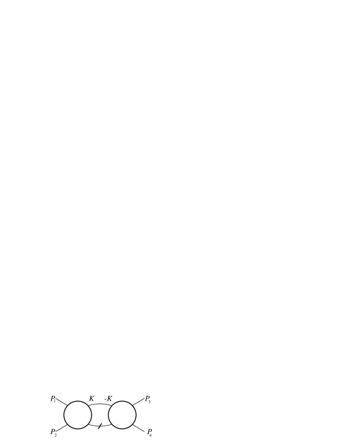
Figure 3: The graph corresponding to $Q_{4,r,2}$

More explicitly, $Q_{4,r,2}$ is given by

$$Q_{4,r,2}(t\mid P_{1}, \mkern-30.0mu\ldots,P_{4})=\frac{1}{2}{\mathbb{A}}_{4}\Big{[}144\sum\limits_{r_{1}+r_{2}=r}\sum\limits_{i_{1},\sigma_{1},i_{2},\sigma_{2}}\int dk\;\bar{D}_{t}(K)\;\dot{\bar{D}_{t}}(K^{\prime})$$ (160)

$$\tilde{I}_{4,r_{1}}(t\mid P_{1},P_{2},K^{\prime},K)\;\tilde{I}_{4,r_{2}}(t\mid\sim K,\sim K^{\prime},P_{3},P_{4})\Big{]}$$

with $K=(k,i_{1},\sigma_{1})$ and $K^{\prime}=(p_{1}+p_{2}-k,i_{2},\sigma_{2})$. Let

$$Q_{4,r,\geq 3}(t\mid\underline{P})=Q_{4,r}(t\mid\underline{P})-Q_{4,r,2}(t\mid\underline{P})$$ (161)

be the contribution from all terms where at least $i\geq 3$ lines connect the two vertices in $Q_{4,r}$. Correspondingly, let

$$\tilde{I}_{4,r}(t)=B_{r}(t)+U_{r}(t)$$ (162)

where $B_{4,r}(t)$ and $U_{4,r}(t)$ are defined by

$$\frac{\partial}{\partial t}B_{r}(t)=\frac{1}{2}{\mathbb{A}}_{4}Q_{4,r,2}(t),\quad\frac{\partial}{\partial t}U_{r}(t)=\frac{1}{2}{\mathbb{A}}_{4}Q_{4,r,\geq 3}(t)$$ (163)

with the initial condition $B_{r}(0)+U_{r}(0)=\tilde{I}_{4,r}(0)$ (where it is understood that one of the two summands on the left hand side is set to zero, see below). Note that because $\tilde{I}_{4,r}$ occurs on the right hand side of both equations in Eq. $(\ref{bubcoup})$, Eq. $(\ref{bubcoup})$ is a coupled system of differential equations.

Definition 3

The function $B^{(L)}_{r}$ obtained from the skeleton RGE by the truncation

$$\frac{\partial}{\partial t}U_{r}(t)=0,\quad U_{r}(0)=0$$ (164)

is the ladder skeleton four-point function. The function $U^{(N)}_{r}$ obtained by the truncation

$$\frac{\partial}{\partial t}B_{r}(t)=0,\quad B_{r}(0)=0$$ (165)

is the non-ladder  skeleton four-point function. The functions $\tilde{I}^{(N)}_{m,r}$, obtained with this truncation, (i.e., where $m_{1}=4$ and $m_{2}=4$ are left out in the sum $\int d\tilde{\kappa}_{4,r}$) are the non-ladder  skeleton Green functions.

The motivation for the split is that in $Q_{4,r,\geq 3}$, the number of internal lines of the graph in Figure 2 is $i\geq 3$, so the volume improvement of Lemmas 7 and 8 improves the power counting.

The constants in the following theorems are independent of $\beta$.

Theorem 3

There is a constant $L_{2}$ such that

$${\left|B^{(L)}_{r}(t)\right|}_{0}\leq{L_{2}}^{r}\;(\frac{1}{2}(1+t))^{r-1}\leq{L_{2}}^{r}\;{\left|\log(\beta\epsilon_{0})\right|}^{r-1}$$ (166)

The series $\sum\limits_{r}B^{(L)}_{r}(t)$ converges uniformly in $t$ and $\underline{P}$ if ${\left|\lambda\log\beta\epsilon_{0}\right|}<{L_{2}}^{-1}$.

Proof:     This follows immediately by induction from Eq. $(\ref{Q4r2def})$ by use of Eq. $(\ref{Xalli})$ with $i=2$ and $\alpha=0$.  

Using one-loop volume bounds one can show that both the particle-particle and the particle-hole ladder are bounded uniformly in $t$ and $\beta$ for ${\bf Q}\neq 0$, so that the only singularity in the four-point function can arise at zero momentum (for a discussion of this, see, e.g., [24]). In the particle-particle ladder, this singularity is really there, and it implies that Fermi liquid behaviour occurs only above a critical temperature: the $\log\beta$ in Definition 1 is the logarithm occurring in Theorem 3.

The next theorem states that the non-ladder  skeleton four-point function is bounded and that consequently, the non-ladder  skeleton selfenergy is $C^{1}$ uniformly in $\beta$. This shows that indeed, only the ladder four-point function produces a nonuniformity in $\beta$ (this motivates the alternative criterion for Fermi liquid behaviour in Section 2.6). The second derivative, however, is only bounded by a power of $\log\beta$ in $d=2$; this motivates why at zero temperature, the self-energy is only required to be $C^{2-\delta}$ for some $\delta>0$.

Theorem 4

For all $r\geq 1$, the non-ladder  skeleton functions $\tilde{I}^{(N)}_{2,r}(t)$ converge for $t\to\infty$ to a $C^{2}$ function. There are constants ${L_{3,r}}$ and ${L_{4,r}}$, independent of $\beta$, such that

$${\left|D^{\alpha}\tilde{I}^{(N)}_{2,r}(t)\right|}_{0}\leq{L_{3,r}}\cases{1&if $|\alpha|\leq 1$\cr(\log\beta\epsilon_{0})^{2}&if $|\alpha|=2$ and $d=2$\cr\log\beta\epsilon_{0}&if $|\alpha|=2$ and $d\geq 3$.}$$ (167)

and

$${\left|D^{\alpha}\tilde{I}^{(N)}_{4,r}(t)\right|}_{0}\leq{L_{4,r}}\cases{1&if $|\alpha|=0$\cr\log\beta\epsilon_{0}&if $|\alpha|=1$\cr\beta\epsilon_{0}&if $|\alpha|=2$.}$$ (168)

If the ladder four-point function is left in the RGE, its logarithmic growth (Theorem 3) shows up in all other Green functions, and in the selfenergy:

Theorem 5

The skeleton functions $\tilde{I}_{2,r}$ and $\tilde{I}_{4,r}$ converge for $t\to\infty$ and satisfy

$${\left|D^{\alpha}\tilde{I}_{m,r}(t)\right|}_{0}\leq{L_{5,m,r}}(\log\beta\epsilon_{0})^{r}$$ (169)

for $m=2$, $|\alpha|\leq 2$, and $m=4$, $|\alpha|=0$.

Theorems 4 and 5 are proven in the next section.

Remark 10

To prove bounds with a good $\beta$ behaviour for $m\geq 6$ requires the use of different norms, where part of the momenta are integrated [19]. It is easy to see that for $m\geq 6$, the connected $m$-point functions have singularities and thus are not uniformly bounded functions of momentum; for instance the second order six-point function is given by $C(P)$, which is $O(\beta)$ if ${\bf p}$ is on the Fermi surface and if $\omega=\pi/\beta$.

Remark 11

A bound $\hbox{ \rm const }^{r}$ for the constants in Theorem 5 would suffice to show the first requirement of the Fermi liquid behaviour defined in Definition 1, namely the convergence of the perturbation expansion for the skeleton functions for ${\left|\lambda\log\beta\right|}<\hbox{ \rm const }$. The proofs given in this section do not imply this bound because in the momentum space equation, the factorial remains. It may, however, be possible to give such bounds in $d=2$ by combining the sector technique of [20] with the determinant bound.

6.3 The regularity proofs

At positive temperature, the frequencies are still discrete, whereas the spatial part of momentum is a continuous variable. Whenever derivatives with respect to $p_{0}$ are written below, they are understood as a difference operation ${\textstyle\frac{\beta}{2\pi}}(f(p_{0}+{\textstyle\frac{2\pi}{\beta}})-f(p_{0}))$. The RGE actually defines the Green functions for (almost all) real values of $p_{0}$, not just the discrete set of Matsubara frequencies, so the effect of such a difference can be bounded by Taylor expansion. This changes at most constants, so I shall not write this out explicitly in the proofs.

The following theorem implies Theorem 4 about the non-ladder  skeleton selfenergy and four-point function. Note that all bounds in this Theorem are independent of $\beta$.

Theorem 6

Let $\alpha$ be a multiindex with $|\alpha|\leq 2$. For all $m,r$, let $I_{mr}(0)$ be $C^{2}$ in $({\bf p}_{1},\ldots,{\bf p}_{m})$, and assume that there are ${K_{mr}^{(0)}}\geq 0$ such that ${\left|D^{\alpha}I_{mr}(0)\right|}\leq{K_{mr}^{(0)}}$, with ${K_{mr}^{(0)}}=0$ for $m>2r+2$, and $K_{m1}^{(0)}=\delta_{m4}v$, where $v>0$. Let $\tilde{I}^{(N)}_{mr}(t)$ be the Green functions generated by the non-ladder  skeleton RGE, as given in Definition 3, with initial values $I_{mr}(0)$. Let $K_{m1}=K_{m1}^{(0)}$ and for $r\geq 2$, let

$$K_{mr}={K_{mr}^{(0)}}+\frac{1}{m}M_{1}\int d\tilde{\kappa}_{mr}i\;i!(32J_{1})^{i-1}K_{m_{1}r_{1}}K_{m_{2}r_{2}}$$ (170)

where $M_{1}=240B{K^{(1)}}$, with $B=\max_{\alpha}B_{\alpha}$. Then $K_{mr}=0$ if $m>2r+2$, and for all $t\geq 0$ and all $m,r$

$${\left|D^{\alpha}\tilde{Q}^{(N)}_{mr}(t)\right|}_{0}\leq 2K_{mr}\cases{\epsilon_{t}^{2-{m\over 2}-|\alpha|}&if $m\geq 6$\cr\epsilon_{t}^{1-|\alpha|}\frac{1+t}{2}&if $m=4$\cr\epsilon_{t}^{2-|\alpha|}\left(\frac{1+t}{2}\right)^{\delta_{d,2}}&if $m=2$.}$$ (171)

Moreover, for $m\geq 6$,

$${\left|D^{\alpha}\tilde{I}^{(N)}_{mr}(t)\right|}_{0}\leq K_{mr}\epsilon_{t}^{2-{m\over 2}-|\alpha|},$$ (172)

for $m=4$

$${\left|D^{\alpha}\tilde{I}^{(N)}_{mr}(t)\right|}_{0}\leq K_{4r}\cases{1&if $\alpha=0$\cr\left(\frac{1+t}{2}\right)^{2}&if $|\alpha|=1$\cr\epsilon_{t}^{-1}\frac{1+t}{2}&if $|\alpha|=2$,}$$ (173)

and for $m=2$

$${\left|D^{\alpha}\tilde{I}^{(N)}_{mr}(t)\right|}_{0}\leq K_{2r}\cases{1&if $|\alpha|\leq 1$\cr\left(\frac{1+t}{2}\right)^{2}&if $|\alpha|=2$ and $d=2$\cr\frac{1+t}{2}&if $|\alpha|=2$ and $d=3$.}$$ (174)

Proof:     Induction in $r$, with the statement of the Theorem as the inductive hypothesis. $r=1$ is trivial because $\tilde{Q}^{(N)}_{m1}=0$ and because the statement holds for $I_{m1}(0)$. Let $r\geq 2$ and the statement hold for all $r^{\prime}<r$. The inductive hypothesis applies to both factors $\tilde{I}^{(N)}_{m_{k}r_{k}}$ in $\tilde{Q}^{(N)}_{mr}$. For $m_{k}=4$, it implies that

$${\left|\tilde{I}^{(N)}_{m_{k}r_{k}}(t)\right|}_{0}\leq K_{m_{k}r_{k}}\epsilon_{t}^{-|\alpha|}=K_{m_{k}r_{k}}\epsilon_{0}^{-|\alpha|}{\rm e}^{t(|\alpha|+{m_{k}\over 2}-2)}$$ (175)

for all $t\geq 0$. Recall Eq. $(\ref{Xalli})$ and Eq. $(\ref{Xige3})$, and

$${\left|D^{\alpha}{\mathbb{A}}_{m}\tilde{Q}^{(N)}_{mr}(t)\right|}_{0} = {\left|{\mathbb{A}}_{m}D^{\alpha}\tilde{Q}^{(N)}_{mr}(t)\right|}_{0}\leq{\left|D^{\alpha}\tilde{Q}^{(N)}_{mr}(t)\right|}_{0}$$ (176)

$$\leq \int d\tilde{\kappa}^{(N)}_{mr}i\;i!{\left|{\cal X}_{\alpha,i}(t)\right|}_{0}.$$

Let $m\geq 6$. By Eq. $(\ref{Xalli})$ and $m_{1}+m_{2}=m+2i$, the $t$-dependent factors in ${\cal X}_{\alpha,i}(t)$ are

$${\rm e}^{t({m_{1}\over 2}-2+|\alpha_{1}|)}\;{\rm e}^{t({m_{2}\over 2}-2+|\alpha_{2}|)}{\rm e}^{t(2-i+|\alpha_{0}|)}={\rm e}^{t({m\over 2}-2+|\alpha|)}$$ (177)

Since $\frac{m}{2}-2+|\alpha|\geq\frac{m}{2}-2\geq 1$, integrating the RGE gives

$${\left|D^{\alpha}\tilde{I}^{(N)}_{mr}(t)\right|}_{0} \leq {\left|D^{\alpha}\tilde{I}^{(N)}_{mr}(0)\right|}_{0}+\frac{1}{2}\int\limits_{0}^{t}ds\;{\left|D^{\alpha}\tilde{Q}^{(N)}_{mr}(s)\right|}_{0}$$ (178)

$$\leq {K_{mr}^{(0)}}+\frac{1}{m-4}\nu_{mr}\epsilon_{t}^{2-{m\over 2}-|\alpha|}$$

where

$$\nu_{mr}=4B\int d\tilde{\kappa}i\;i!(32J_{1})^{i-1}\sum\limits_{\underline{\alpha}}{\textstyle\frac{\alpha!}{\alpha_{0}!\alpha_{1}!\alpha_{2}!}}K_{m_{1}r_{1}}K_{m_{2}r_{2}}.$$ (179)

For $m\geq 6$, $m-4\geq\frac{m}{3}$. Moreover, $\sum{\textstyle\frac{\alpha!}{\alpha_{0}!\alpha_{1}!\alpha_{2}!}}\leq 3^{|\alpha|}$, so Eq. $(\ref{iha})$ and Eq. $(\ref{ihb6})$ follow.

Let $m=4$. One of $m_{1}$ and $m_{2}$ must be at least six because the ladder part is left out in $\tilde{I}^{(N)}_{mr}$. Thus $i=\frac{1}{2}(m_{1}+m_{2}-4)\geq 3$. By Eq. $(\ref{Xige3})$, there is an extra small factor $\epsilon_{t}=\epsilon_{0}{\rm e}^{-t}$, so

$${\left|D^{\alpha}\tilde{Q}^{(N)}_{4,r}(t)\right|}_{0}\leq\frac{1+t}{2}\epsilon_{t}^{1-|\alpha|}\;{K^{(1)}}\nu_{mr},$$ (180)

which proves Eq. $(\ref{iha})$. Eq. $(\ref{ihb4})$ follows by integration.

Let $m=2$. The case $m_{1}=m_{2}=2$ is excluded since this is the skeleton RG. Thus $i=\frac{1}{2}(m_{1}+m_{2}-2)\geq 3$, and Eq. $(\ref{Xige3})$ implies

$${\left|D^{\alpha}\tilde{Q}^{(N)}_{2,r}(t)\right|}_{0}\leq\left(\frac{1+t}{2}\right)^{\delta_{d,2}}\;\epsilon_{t}^{1-|\alpha|}\;{K^{(1)}}\nu_{2r}.$$ (181)

Thus Eq. $(\ref{iha})$ holds, and Eq. $(\ref{ihb2})$ follows by integration.  

Proof:    [of Theorem 4] Let $|\alpha|\leq 1$. By Eq. $(\ref{ihb2})$, $|D^{\alpha}\tilde{I}^{(N)}_{2r}(t)|\leq K_{2,r}$. By Eq. $(\ref{iha})$, $|D^{\alpha}{\textstyle\frac{\partial}{\partial t}}\tilde{I}^{(N)}_{2r}(t)|\leq K_{2,r}\epsilon_{0}{\rm e}^{-t}\;{\textstyle\frac{1+t}{2}}\to 0$ as $t\to\infty$. Thus the limit $t\to\infty$ of $\tilde{I}^{(N)}_{2,r}(t)$ exists and is a $C^{1}$ function of $({\bf p}_{1},{\bf p}_{2})$. All constants are uniform in $\beta$. The second derivative of $\tilde{Q}^{(N)}_{2,r}$ is $O(t)$ in $d=2$ and $O(1)$ in $d=3$. Since $\tilde{Q}^{(N)}_{2,r}=0$ for $t>\log\beta\epsilon_{0}$, the integral for $\tilde{I}^{(N)}_{2,r}$ over $t$ runs only up to $\log\beta\epsilon_{0}$, which gives the stated dependence on $\log\beta\epsilon_{0}$.  

Remark 12

Note that the bounds for $m=2$ and $|\alpha|=2$ in Theorem 6 do not imply convergence. This is the source of the logarithmic behaviour discussed in Section 2.6 and in [22].

The following theorem implies Theorem 5. Here the bounds have an explicit $\beta$-dependence. One could avoid this $\beta$-dependence by including polynomials in $t$, but this would also increase the combinatorial coefficients by factorials.

Theorem 7

Let $\alpha$ be a multiindex with $|\alpha|\leq 2$. For all $m,r$, let $I_{mr}(0)$ be $C^{2}$ in $({\bf p}_{1},\ldots,{\bf p}_{m})$, and assume that there are ${K_{mr}^{(0)}}\geq 0$ such that ${\left|D^{\alpha}I_{mr}(0)\right|}\leq{K_{mr}^{(0)}}$, with ${K_{mr}^{(0)}}=0$ for $m>2r+2$, and $K_{m1}^{(0)}=\delta_{m4}v$, where $v>0$. Let $\tilde{I}_{mr}(t)$ be the Green functions generated by the skeleton RGE, as given in Definition 2, with initial values $I_{mr}(0)$. Let $K_{m1}=K_{m1}^{(0)}$ and for $r\geq 2$, let $K_{mr}$ be given by Eq. $(\ref{kKmrdef})$. Then for $m\geq 4$

$${\left|D^{\alpha}\tilde{Q}_{mr}(t)\right|}_{0}\leq 2K_{mr}\;(\log\beta\epsilon_{0})^{r-2}\epsilon_{t}^{2-{m\over 2}-|\alpha|}$$ (182)

and

$${\left|D^{\alpha}\tilde{I}_{mr}(t)\right|}_{0}\leq K_{mr}\;(\log\beta\epsilon_{0})^{r-1}\epsilon_{t}^{2-{m\over 2}-|\alpha|}.$$ (183)

For $m=2$,

$${\left|D^{\alpha}\tilde{Q}_{2r}(t)\right|}_{0}\leq 2K_{2r}\;(\log\beta\epsilon_{0})^{r-2+\delta_{d,2}}\epsilon_{t}^{2-|\alpha|}$$ (184)

and

$${\left|D^{\alpha}\tilde{I}_{2r}(t)\right|}_{0}\leq K_{2r}\;(\log\beta\epsilon_{0})^{r-2}\cases{1&if $|\alpha|\leq 1$\cr(\log\beta\epsilon_{0})^{1+\delta_{d,2}}&if $|\alpha|=2$.}$$ (185)

Proof:     The proof is by induction in $r$, with the statement of the theorem as the inductive hypothesis. It is similar to the proof of Theorem 6, with only a few changes. Note that $m_{1}=2$ and $m_{2}=2$ never appear on the right hand side of the RGE because of the skeleton truncation in Definition 2. For $m\geq 4$, use Eq. $(\ref{Xalli})$; this gives

$${\left|D^{\alpha}\tilde{Q}_{mr}(t)\right|}_{0}\leq 9\nu_{mr}\;(\log\beta\epsilon_{0})^{r-2}\;\epsilon_{t}^{2-{m\over 2}-|\alpha|}.$$ (186)

For $m\geq 6$, the scale integral is as in the proof of Theorem 6. For $m=4$, the scale integral is now $\int_{0}^{t}ds\;=t\leq\log\beta\epsilon_{0}$. This produces the powers of $\log\beta\epsilon_{0}$ upon iteration. For $m\geq 2$, use Eq. $(\ref{Xige3})$; this gives ${K^{(1)}}\epsilon_{t}^{2-|\alpha|}(\frac{1}{2}(1+t))^{\delta_{d,2}}$ instead of $\epsilon_{t}^{2-{m\over 2}-|\alpha|}$ in Eq. $(\ref{47stro})$. The theorem now follows by integration over $t$, recalling that the upper integration limit is at most $\log\beta\epsilon_{0}$.  

Proof:     [ of Theorem 5] Convergence of the selfenergy follows for $|\alpha|\leq 1$ as in the proof of Theorem 4. For $m=4$, the function is bounded uniformly in $t$. For $|\alpha|=2$, convergence at $\beta>0$ holds because ${\textstyle\frac{\partial}{\partial t}}\tilde{I}_{4r}(t)=0$ for $t>\log\beta\epsilon_{0}$.  

7 Conclusion

The determinant bound for the continuous Wick-ordered RGE removes a factorial in the recursion for the Green functions. If the model has a propagator with a pointlike singularity, power counting bounds that include this combinatorial improvement can be proven rather easily. The improvement may lead to convergence, but I have not proven this here. If it does, then Theorem 1 implies analyticity of the Green functions where all relevant and marginal couplings are left out in a region independent of the energy scale, and Theorem 2 implies analyticity of the full Green functions for $|\lambda|\beta^{d}<\hbox{ \rm const }$ in many-fermion systems for all $d\geq 1$. Natural models to which Theorem 1 applies are the Gross-Neveu model in two dimensions and the many-fermion system in one dimension. In both cases, I have only given bounds where the marginal and relevant terms where left out, to give a simple application of the determinant bound derived in Section 4. In both cases, analyses of the full models, including the coupling flows, have been done previously ([14, 15] and [16, 17, 18]).

Many-fermion models in $d\geq 2$ are the most realistic physical systems where the interaction is regular enough for the analysis done here to apply directly (i.e., without the introduction of boson fields). I have defined a criterion for Fermi liquid behaviour for these models. A proof that such behaviour occurs requires more detailed bounds and a combination of the method with the sector method of [20]. This may be feasible by an extension of the analysis done here. The Jellium dispersion relation $E({\bf k})={\bf k}^{2}/2-\mu$ is the case where the proofs are easiest because $\Sigma|_{\cal S}$ is constant. The proof that such a system is a Fermi liquid is possible by a combination of the techniques of [20] and [21]; is may also be within the reach of the continuous RGE method developed here. Perturbative bounds that implement the overlapping loop method of [21] in a simple way were given in Section 6.

The verification of regularity property $(2)$ for nonspherical Fermi surfaces is not as simple, but the perturbative analysis done here can be extended rather easily to include the double overlaps used in [23], because the graph classification of [23] arises in a natural way when the integral equation for the effective action is iterated. Multiple overlaps can also be exploited in the RGE; this may be necessary for the many-fermion systems in $d\geq 3$. The split of the four-point function into the ladder and non-ladder  part done in Section 6.2 singles out the only singular contributions to the four-point function and the least regular contributions to the self-energy in a simple way. The treatment of these ladder contributions was done in [22], where bounds uniform in the temperature were shown for the second derivative in perturbation theory.

The results in Section 6.2 provide another proof that only the ladder flow corresponding to Figure 3 leads to singularities and hence instabilities. It should be noted that this statement depends on the assumptions stated in Section 2.3, in particular on the choice of $\epsilon_{0}$, in the following specific way. The curvature of the Fermi surface sets a natural scale which appears via the constants in the volume bounds. Above this scale, the geometry of the Fermi surface provides no justification of restricting to the ladder flow. This is of some relevance in the Hubbard model, where two scale regimes arise in a natural way: if $\epsilon_{t}>\tilde{\mu}$, where $\tilde{\mu}=\mu-{\rm t}d$, $t$ the hopping parameter, is defined such that $\tilde{\mu}=0$ is half-filling, then the curvature of the Fermi surface is effectively so small that one can replace the Fermi surface by a square. More technically speaking, the constant $Q_{V}$, which depends on the curvature of the Fermi surface, diverges for $\tilde{\mu}\to 0$. Thus, for small $\tilde{\mu}$, $\epsilon_{t}$ has to be very small for $Q_{V}\epsilon_{t}<1$ to hold. If $Q_{V}\epsilon_{t}>1$, the improved volume estimate does not lead to a gain over ordinary power counting. Only below this energy scale, the curvature effects of the volume improvement bound, Lemma 6, imply domination of the ladder part of the four-point function. To get to scale $\tilde{\mu}$, one has to calculate the effective action. Needless to say, the effective four-point interaction at scale $\tilde{\mu}$ may look very different from the original interaction, and RPA calculations suggest that the antiferromagnetic correlations produced by the almost square Fermi surface lead to an attractive nearest-neighbour-interaction [37]. However, one should keep in mind that for the reasons just mentioned, it is an ad hoc approximation to keep only the RPA part of the four-point function above scale $\tilde{\mu}$, and that a correct treatment must either give a different justification of the ladder approximation, or replace it by a better controlled approximation.

Above, I have not discussed how one gets from the skeleton Green functions to the exact Green functions. The key to this is to take a Wick ordering covariance which already contains part of the self-energy. That is, the Gaussian measure changes in a nontrivial way with $t$. This can be done such that all two-legged insertions appear with the proper renormalization subtractions, and it gives a simple procedure for a rigorous skeleton expansion. Moreover, it makes clear why it is so important to establish regularity of the self-energy: once the self-energy appears in the propagator, its regularity is needed to show Lemma 4 (or its sector analogue), on which in turn, all other bounds depend. The condition ${k_{0}}>d$ also enters in this lemma and seems indispensable from the point of view of the method developed here. Details about this modified Wick ordering technique will appear later.

There is a basic duality in the technique applied to these fermionic models. The determinant bound has to be done in position space, but the regularity bounds use geometric details that are most easily seen in momentum space. The continuous RGE shows very nicely that those terms that require the very detailed regularity analysis are very simple from the combinatorial point of view and vice versa.

Appendix A Fourier transformation

Recall that $\psi$ is defined on the doubled time direction ${\mathbb{T}}_{2}$ and obeys the antiperiodicity with respect to translations by $\beta$, Eq. $(\ref{psanti})$, and that $n_{\tau}$ was chosen to be even. ${\mathbb{T}}_{2}$ is the set ${\mathbb{T}}_{2}=\varepsilon_{\tau}{\mathbb{Z}}/2\beta{\mathbb{Z}}={\mathbb{T}}\cup({\mathbb{T}}+\beta)$ where

$${\mathbb{T}}=\{\tau\in{\mathbb{T}}_{2}:\tau=\varepsilon_{\tau}k,\;k\in\{-\frac{n_{\tau}}{2},\ldots,\frac{n_{\tau}}{2}-1\}\}.$$ (187)

The dual to ${\mathbb{T}}_{2}$ is ${\mathbb{T}}_{2}^{*}=\frac{\pi}{\beta}{\mathbb{Z}}/2n_{\tau}{\mathbb{Z}}=\{\omega=\frac{\pi}{\beta}k:\;k\in\{-n_{\tau},\ldots,n_{\tau}-1\}\}$. The Fourier transform on ${\mathbb{T}}_{2}$ is

$$\tilde{f}(\omega)=\varepsilon_{\tau}\sum\limits_{\tau\in{\mathbb{T}}_{2}}{\rm e}^{-{\rm i}\omega\tau}f(\tau),\quad f(\tau)=\frac{1}{2\beta}\sum\limits_{\omega\in{\mathbb{T}}_{2}}{\rm e}^{{\rm i}\omega\tau}\tilde{f}(\omega).$$ (188)

If $f(\tau-\beta)=-f(\tau)$, then $\tilde{f}(\omega)=0$ if $\frac{\omega\beta}{\pi}$ is even. In that case, with $\hat{f}(\omega)=\frac{1}{2}\tilde{f}(\omega)$,

$$f(\tau)=\frac{1}{\beta}\sum\limits_{\omega\in{\mathbb{M}}_{n_{\tau}}}{\rm e}^{{\rm i}\omega\tau}\hat{f}(\omega)$$ (189)

with ${\mathbb{M}}_{n_{\tau}}$ given by Eq. $(\ref{Matsdef})$. The orthogonality relations are

$$\int\limits_{{\mathbb{T}}}d\tau\;{\rm e}^{{\rm i}(\omega_{n}\pm\omega_{m})\tau}=\beta\delta_{mn},\quad\frac{1}{\beta}\sum\limits_{\omega\in{\mathbb{M}}_{n_{\tau}}}{\rm e}^{{\rm i}\omega\tau}=\frac{1}{\varepsilon_{\tau}}(\delta_{\tau 0}-\delta_{\tau\beta}).$$ (190)

Lemma 9

Let $\beta>0$, $E_{0}\geq 0$, and $n_{\tau}\geq 2\beta(E_{0}+E_{\rm max})$, where $E_{\rm max}$ is defined in Eq. $(\ref{EMAX})$, and let $\widehat{\omega}$ be defined as in Eq. $(\ref{Hatomdef})$. Then for all ${\bf k}\in{\cal B}$ and all $\omega\in{\mathbb{M}}_{n_{\tau}}$, $|{\rm i}\widehat{\omega}-E({\bf k})|\leq E_{0}$ implies $|\omega|\leq{\textstyle\frac{\pi}{2}}E_{0}$ and $|E({\bf k})|\leq 2E_{0}$, and

$${\textstyle\frac{1}{\beta}}\sum\limits_{\omega\in{\mathbb{M}}_{n_{\tau}}}\;{\mathchoice{\rm 1\mskip-4.0mul}{\rm 1\mskip-4.0mul}{\rm 1\mskip-4.5mul}{\rm 1\mskip-5.0mul}}\left(|{\rm i}\widehat{\omega}-E({\bf k})|\leq E_{0}\right)\;\leq E_{0}\;{\mathchoice{\rm 1\mskip-4.0mul}{\rm 1\mskip-4.0mul}{\rm 1\mskip-4.5mul}{\rm 1\mskip-5.0mul}}\left(|E({\bf k})|\leq 2E_{0}\right)\;.$$ (191)

Proof:     By Eq. $(\ref{Hatomdef})$, $\mbox{Im }\widehat{\omega}={\textstyle\frac{1}{\varepsilon_{\tau}}}(1-\cos(\omega\varepsilon_{\tau}))$ and $\mbox{ Re }\widehat{\omega}={\textstyle\frac{1}{\varepsilon_{\tau}}}\sin(\omega\varepsilon_{\tau})$. The condition $|{\rm i}\widehat{\omega}-E({\bf k})|\leq E_{0}$ implies $|\mbox{Re }\widehat{\omega}|\leq E_{0}$ and $|\mbox{Im }\widehat{\omega}+E({\bf k})|\leq E_{0}$. Thus $|\mbox{Im }\widehat{\omega}|\leq E_{0}+E_{\rm max}$. Since $1-\cos x\geq{\textstyle\frac{2}{\pi^{2}}}x^{2}$, $(E_{0}+E_{\rm max})\varepsilon_{\tau}\geq\varepsilon_{\tau}|\mbox{Im }\widehat{\omega}|=1-\cos(\omega\varepsilon_{\tau})\geq{\textstyle\frac{2}{\pi^{2}}}(\omega\varepsilon_{\tau})^{2}$, so $|\omega\varepsilon_{\tau}|\leq\pi(\beta(E_{0}+E_{\rm max})(2n_{\tau})^{-1})^{1/2}\leq{\textstyle\frac{\pi}{2}}$. Since ${\textstyle\frac{\sin x}{x}}$ is decreasing on $[0,{\textstyle\frac{\pi}{2}}]$, $E_{0}\geq|\mbox{Re }\widehat{\omega}|\geq|\omega||{\textstyle\frac{\sin(\omega\varepsilon_{\tau})}{\omega\varepsilon_{\tau}}}|\geq{\textstyle\frac{2}{\pi}}|\omega|$. So $|\omega|\leq{\textstyle\frac{\pi}{2}}E_{0}$. Since $1-\cos x\leq{\textstyle\frac{1}{2}}x^{2}$,

$${\left|\mbox{Im }\widehat{\omega}\right|}\leq{\textstyle\frac{1}{2\varepsilon_{\tau}}}(\omega\varepsilon_{\tau})^{2}\leq\frac{\pi^{2}}{8}\beta E_{0}^{2}\frac{1}{n_{\tau}}\leq E_{0}.$$ (192)

Thus $|\mbox{Im }\widehat{\omega}+E({\bf k})|\leq E_{0}$ implies $|E({\bf k})|\leq 2E_{0}$. In terms of indicator functions, this means that $\;{\mathchoice{\rm 1\mskip-4.0mul}{\rm 1\mskip-4.0mul}{\rm 1\mskip-4.5mul}{\rm 1\mskip-5.0mul}}\left(|{\rm i}\widehat{\omega}-E({\bf k})|\leq E_{0}\right)\;\leq\;{\mathchoice{\rm 1\mskip-4.0mul}{\rm 1\mskip-4.0mul}{\rm 1\mskip-4.5mul}{\rm 1\mskip-5.0mul}}\left(|\omega|\leq{\textstyle\frac{\pi}{2}}E_{0}\right)\;\;{\mathchoice{\rm 1\mskip-4.0mul}{\rm 1\mskip-4.0mul}{\rm 1\mskip-4.5mul}{\rm 1\mskip-5.0mul}}\left(|E({\bf k})|\leq 2E_{0}\right)\;$. The summation over ${\mathbb{M}}_{n_{\tau}}$ gives

$${\textstyle\frac{1}{\beta}}\sum\limits_{\omega\in{\mathbb{M}}_{n_{\tau}}}\;{\mathchoice{\rm 1\mskip-4.0mul}{\rm 1\mskip-4.0mul}{\rm 1\mskip-4.5mul}{\rm 1\mskip-5.0mul}}\left(|\omega|\leq{\textstyle\frac{\pi}{2}}E_{0}\right)\;={\textstyle\frac{1}{\beta}}\sum\limits_{n=-{n_{\tau}\over 2}}^{n_{\tau}\over 2}\;{\mathchoice{\rm 1\mskip-4.0mul}{\rm 1\mskip-4.0mul}{\rm 1\mskip-4.5mul}{\rm 1\mskip-5.0mul}}\left(|2n+1|\leq{\textstyle\frac{\beta E_{0}}{2}}\right)\;\leq E_{0}.$$ (193)

Note that the last inequality holds in particular if ${\textstyle\frac{\beta E_{0}}{2}}<1$, because then the sum is empty, hence the result zero, because $2n+1$ is always odd.  

Appendix B Wick ordering

Recall the conventions fixed at the beginning of Section 3.

Definition 4

Let ${\cal W}_{\Gamma}(\eta,\psi)={\rm e}^{(\eta,\psi)_{\Gamma}-\frac{1}{2}(\eta,\,C\,\eta)_{\Gamma}}$, and let ${\cal A}_{\Gamma}^{\prime}$ be the Grassmann algebra generated by $(\psi(x))_{x\in\Gamma}$. Wick ordering is the ${\mathbb{C}}$–linear map $\Omega_{C}:{\cal A}_{\Gamma}^{\prime}\to{\cal A}_{\Gamma}^{\prime}$ that takes the following values on the monomials: $\Omega_{C}(1)=1$, and for $n\geq 1$ and $X_{1},\ldots,X_{n}\in\Gamma$,

$$\Omega_{C}\big{(}\psi(X_{1})\ldots\psi(X_{n})\big{)}=\left[\prod\limits_{k=1}^{n}\frac{\delta}{\delta\eta(X_{k})}\;{\cal W}_{\Gamma}(\eta,\psi)\right]_{\eta=0}$$ (194)

Theorem 8

${\cal W}_{\Gamma}(\eta,\psi)=\Omega_{C}\left({\rm e}^{(\eta,\psi)_{\Gamma}}\right)$. Let $\alpha_{1},\ldots,\alpha_{n}$ be Grassmann variables, and let $\alpha(X)=\sum_{k=1}^{n}\alpha_{k}\;\delta_{\Gamma}(X,X_{k})$. Then

$$\Omega_{C}\big{(}\psi(X_{1})\ldots\psi(X_{n})\big{)}=\left[\left(\prod\limits_{k=1}^{n}\frac{\partial}{\partial\alpha_{k}}\right)\Omega_{C}\left({\rm e}^{(\alpha,\psi)_{\Gamma}}\right)\right]_{\alpha=0}$$ (195)

Proof:     By Taylor expansion in $\eta$, and by definition of $\Omega_{C}$,

$${\cal W}_{\Gamma}(\eta,\psi) = \sum\limits_{n\geq 0}\frac{1}{n!}\;\sum\limits_{X_{1},\ldots,X_{n}\in\Gamma}\left[\prod\limits_{k=1}^{n}\eta(X_{k})\frac{\partial}{\partial\alpha(X_{k})}\;{\cal W}_{\Gamma}(\alpha,\psi)\right]_{\alpha=0}$$ (196)

$$= \sum\limits_{n\geq 0}\frac{1}{n!}\;\int dX_{1}\ldots dX_{n}\;\left[\prod\limits_{k=1}^{n}\eta(X_{k})\frac{\delta}{\delta\alpha(X_{k})}\;{\cal W}_{\Gamma}(\alpha,\psi)\right]_{\alpha=0}$$

$$= \sum\limits_{n\geq 0}\frac{1}{n!}\;\int dX_{1}\ldots dX_{n}\;\Omega_{C}\left(\prod\limits_{k=1}^{n}\eta(X_{k})\psi(X_{k})\right)$$

$$= \sum\limits_{n\geq 0}\frac{1}{n!}\;\Omega_{C}\left({(\eta,\psi)_{\Gamma}}^{n}\right)=\Omega_{C}\left({\rm e}^{(\eta,\psi)_{\Gamma}}\right).$$

Eq. $(\ref{nuetzli})$ follows directly from the definition of $\Omega_{C}$.  

The next theorem contains the alternative formula Eq. $(\ref{WiLa})$ for the Wick ordered monomials used in Section 2.

Theorem 9

Let $\Delta_{C_{t}}$ be defined by Eq. $(\ref{LpCtdef})$. Then

$$\Omega_{C_{t}}\big{(}\psi(X_{1})\ldots\psi(X_{n})\big{)}={\rm e}^{-\Delta_{C_{t}}}\;\psi(X_{1})\ldots\psi(X_{n}).$$ (197)

In particular, if $C_{t}$ depends differentiably on $t$, then

$$\frac{\partial}{\partial t}\Omega_{C_{t}}\big{(}\psi(X_{1})\ldots\psi(X_{n})\big{)}=-\frac{\partial\Delta_{C_{t}}}{\partial t}\Omega_{C}\big{(}\psi(X_{1})\ldots\psi(X_{n})\big{)}$$ (198)

Proof:     For any formal power series $f(z)=\sum f_{k}z^{k}$,

$$f(\Delta_{C_{t}})\;{\rm e}^{(\eta,\psi)_{\Gamma}}=f\left(\frac{1}{2}(\eta\;,C_{t}\;\eta)_{\Gamma}\right)\;{\rm e}^{(\eta,\psi)_{\Gamma}},$$ (199)

so ${\rm e}^{-\Delta_{C_{t}}}\;{\rm e}^{(\eta,\psi)_{\Gamma}}={\rm e}^{-\frac{1}{2}(\eta,C_{t}\eta)_{\Gamma}+(\eta,\psi)_{\Gamma}}$, from which Eq. $(\ref{altrep})$ follows by definition of $\Omega_{C_{t}}$, because derivatives with respect to $\eta$ commute with $\Delta_{C_{t}}$. If $C_{t}$ depends differentiably on $t$, Eq. $(\ref{Lapder})$ follows by taking a derivative of Eq. $(\ref{altrep})$ because $\Delta_{C_{t}}$ commutes with $\frac{\partial\Delta_{C_{t}}}{\partial t}$.  

Appendix C Wick reordering

By Eq. $(\ref{expaWO})$ and Eq. $(\ref{toWm})$, ${\cal Q}_{r}(t,\psi)={\textstyle\frac{1}{2}}\sum\limits_{r_{1}\geq 1,r_{2}\geq 1\atop r_{1}+r_{2}=r}\sum\limits_{m_{1}=1}^{\bar{m}(r_{1})}\sum\limits_{m_{2}=1}^{\bar{m}(r_{2})}{\cal Y}_{r_{1},m_{1},r_{2},m_{2}}$ with

$${\cal Y}_{r_{1},m_{1},r_{2},m_{2}}=\int d\underline{X}\;G_{m_{1}r_{1}}(t\mid\underline{X}^{(1)})\;G_{m_{2}r_{2}}(t\mid\underline{X}^{(2)})\;P(\underline{X},\psi)$$ (200)

where $\underline{X}^{(1)}=(X_{1},\ldots,X_{m_{1}})$, $\underline{X}^{(2)}=(X_{m_{1}+1},\ldots,X_{m_{1}+m_{2}})$, $\underline{X}=(X_{1},\ldots,$ $X_{m_{1}+m_{2}})$, $P(\underline{X},\psi)=\int dXdY\dot{C}_{t}(X,Y)\;\omega_{X,Y}(\psi)$, and

$$\omega_{X,Y}(\psi)=\left(\frac{\delta}{\delta\psi(X)}\Omega_{D_{t}}\left(\prod\limits_{k_{1}=1}^{m_{1}}\psi(X_{k_{1}})\right)\right)\;\frac{\delta}{\delta\psi(Y)}\Omega_{D_{t}}\left(\prod\limits_{k_{2}=1}^{m_{2}}\psi(X_{m_{1}+k_{2}})\right).$$ (201)

Only even $m_{1}$ and $m_{2}$ contribute to the sum for ${\cal Q}_{r}(t,\psi)$ because ${\cal G}_{r}(t,\psi)$ is an element of the even subalgebra for all $t$. Let

$$\eta^{(1)}=\sum\limits_{k=1}^{m_{1}}\eta_{k}\;\delta_{\Gamma}(X,X_{k}),\quad\eta^{(2)}=\sum\limits_{k=1}^{m_{2}}\eta_{m_{1}+k}\;\delta_{\Gamma}(X,X_{m_{1}+k}),\quad$$ (202)

and $\eta=\eta^{(1)}+\eta^{(2)}$. With this,

$$\frac{\delta}{\delta\psi(X)}\Omega_{D_{t}} \kern-26.0pt\left(\prod\limits_{k_{1}=1}^{m_{1}}\psi(X_{k_{1}})\right)=\left[\frac{\delta}{\delta\psi(X)}\prod\limits_{k=1}^{m_{1}}\frac{\partial}{\partial\eta_{k}}\Omega_{D_{t}}\left({\rm e}^{(\eta^{(1)},\psi)_{\Gamma}}\right)\right]_{\eta=0}$$ (203)

$$= (-1)^{m_{1}}\left[\prod\limits_{k=1}^{m_{1}}\frac{\partial}{\partial\eta_{k}}\frac{\delta}{\delta\psi(X)}{\rm e}^{(\eta^{(1)},\psi)_{\Gamma}-\frac{1}{2}(\eta^{(1)},D_{t}\eta^{(1)})_{\Gamma}}\right]_{\eta=0}$$

$$= \left[\prod\limits_{k=1}^{m_{1}}\frac{\partial}{\partial\eta_{k}}(-1)\eta^{(1)}(X){\rm e}^{(\eta^{(1)},\psi)_{\Gamma}-\frac{1}{2}(\eta^{(1)},D_{t}\eta^{(1)})_{\Gamma}}\right]_{\eta=0}$$

since $(-1)^{m_{1}}=1$. Similarly,

$$\Omega_{D_{t}}\left(\prod\limits_{k=1}^{m_{2}}\psi(X_{k})\right)=\left[\prod\limits_{k=1}^{m_{2}}\frac{\partial}{\partial\eta_{m_{1}+k}}(-1)\eta^{(2)}(Y){\rm e}^{(\eta^{(2)},\psi)_{\Gamma}-\frac{1}{2}(\eta^{(2)},D_{t}\eta^{(2)})_{\Gamma}}\right]_{\eta=0}$$ (204)

Since $\eta^{(1)}$ is independent of $\eta_{m_{1}+1},\ldots,\eta_{m_{1}+m_{2}}$, the derivatives with respect to $\eta^{(2)}$ can be commuted through so that

$$P(\underline{X},\psi)=\left[\frac{\partial^{m_{1}+m_{2}}}{\partial\eta_{1}\ldots\partial\eta_{m_{1}+m_{2}}}\;Z(\eta,\psi)\right]_{\eta=0}$$ (205)

with

$$Z(\eta,\psi)=(\eta^{(1)},\;\dot{C}_{t}\;\eta^{(2)})\;{\rm e}^{(\eta,\psi)_{\Gamma}-\frac{1}{2}(\eta^{(1)},\;D_{t}\;\eta^{(1)})_{\Gamma}-\frac{1}{2}(\eta^{(2)},\;D_{t}\;\eta^{(2)})_{\Gamma}}$$ (206)

Wick ordering of ${\rm e}^{(\eta,\psi)_{\Gamma}}$, the antisymmetry of $D_{t}$, and $\dot{C}_{t}=-\dot{D}_{t}$, give

$$Z(\eta,\psi)=\left(-\;{\textstyle\frac{\partial}{\partial t}}\;{\rm e}^{(\eta^{(1)},\;D_{t}\;\eta^{(2)})_{\Gamma}}\right)\Omega_{D_{t}}\left({\rm e}^{(\eta,\psi)_{\Gamma}}\right).$$ (207)

Lemma 10

Let $A$ and $B$ be elements of the Grassmann algebra generated by $(\eta(X))_{X\in\Gamma}$, that is, $A=\sum_{I\subset\Gamma}a_{I}\;\eta^{I}$ and $B=\sum_{I\subset\Gamma}b_{I}\;\eta^{I}$, where $a_{I},b_{I}\in{\mathbb{C}}$, and let $F(x)$ be the formal power series $F(x)=\sum_{r\geq 0}f_{r}x^{r}$. Then

$$\left[A(\frac{\partial}{\partial\eta})\;B(\eta)\;F\big{(}(\eta,\psi)\big{)}\right]_{\eta=0}=\left[A(\eta)\;B(\frac{\partial_{L}}{\partial\eta})\;F\big{(}(\frac{\partial_{L}}{\partial\eta},\psi)\big{)}\right]_{\eta=0}$$ (208)

where $\frac{\partial_{L}}{\partial\eta}$ is the derivative with respect to $\eta$, acting to the left.

Proof:     The proof is an easy exercise in Grassmann algebra and is left to the reader.  

Let $m_{1}+m_{2}=\mu$. By Lemma 10

$$\left[\frac{\partial^{\mu}}{\partial\eta_{1}\ldots\partial\eta_{\mu}}\;Z(\eta,\psi)\right]_{\eta=0}=\left[\eta_{1}\ldots\eta_{\mu}\;Z(\frac{\partial_{L}}{\partial\eta},\psi)\right]_{\eta=0}$$ (209)

By definition of $\eta^{(1)}$ and $\eta^{(2)}$,

$$\left(\frac{\partial_{L}}{\partial\eta^{(1)}},D_{t}\frac{\partial_{L}}{\partial\eta^{(2)}}\right)=\sum\limits_{k_{1}=1}^{m_{1}}\sum\limits_{k_{2}=m_{1}+1}^{\mu}\frac{\partial_{L}}{\partial\eta_{k_{1}}}D_{t}(X_{k_{1}},X_{k_{2}})\frac{\partial_{L}}{\partial\eta_{k_{2}}}.$$ (210)

Every derivative can act only once on $\eta_{1}\ldots\eta_{\mu}$ without giving zero because the $\eta$’s are all different. So

$$\eta_{1}\ldots\eta_{\mu} \kern-20.0pt\exp\left(\frac{\partial_{L}}{\partial\eta^{(1)}},D_{t}\frac{\partial_{L}}{\partial\eta^{(2)}}\right)$$ (211)

$$= \sum\limits_{L\subset M_{1}\times M_{2}}\eta_{1}\ldots\eta_{\mu}\prod\limits_{(k_{1},k_{2})\in L}\left(\frac{\partial_{L}}{\partial\eta_{k_{1}}}D_{t}(X_{k_{1}},X_{k_{2}})\frac{\partial_{L}}{\partial\eta_{k_{2}}}\right)$$

where $M_{1}=\{1,\ldots,m_{1}\}$ and $M_{2}=\{m_{1}+1,\ldots,\mu\}$. $L=\emptyset$ contributes to the sum, but gives the $t$-independent result $\eta_{1}\ldots\eta_{\mu}$, so the $t$-derivative removes this term in Eq. $(\ref{Z3})$. Let $\pi_{1}(k_{1},k_{2})=k_{1}$ and $\pi_{2}(k_{1},k_{2})=k_{2}$. For a term given by $L\neq\emptyset$ to be nonzero, $\pi_{1}|_{L}$ and $\pi_{2}|_{L}$ must be injective, because otherwise a derivative would act twice. Thus the sum can be restricted to the set

$${\cal L}=\{L\subset M_{1}\times M_{2}:L\neq\emptyset,\mbox{ and }\pi_{k}\mid_{L}\mbox{ injective for }k=1,2\}$$ (212)

If $L\in{\cal L}$, $\pi_{1}(L)=\pi_{2}(L)$. Thus

$${\cal L}=\bigcup\limits_{i=1}^{\min\{m_{1},m_{2}\}}\;\bigcup\limits_{B_{i}\subset M_{i}\atop|B_{1}|=|B_{2}|=i}{\cal L}(B_{1},B_{2})$$ (213)

with

$${\cal L}(B_{1},B_{2})=\{L\in{\cal L}:\pi_{1}(L)=B_{1}\mbox{ and }\pi_{2}(L)=B_{2}\}.$$ (214)

Let

$$B_{1}=\{b_{1},\ldots,b_{i}\}, 1\leq b_{1}<\ldots b_{i}\leq m_{1},$$

$$B_{2}=\{b_{i+1},\ldots,b_{2i}\}, m_{1}+1\leq b_{i+1}<\ldots b_{2i}\leq m_{1}+m_{2},$$ (215)

then for any $L\in{\cal L}(B_{1},B_{2})$, there is a unique permutation $\pi\in{\cal S}_{i}$ such that

$$L=\{(b_{k},b_{i+\pi(k)}):k\in\{1,\ldots,i\}\}.$$ (216)

Thus the sum over $L$ splits into a sum over $i\geq 1$, a sum over sequences $b=(b_{1},\ldots,b_{2i})$ with

$$1\leq b_{1}<b_{2}<\ldots<b_{i}\leq m_{1}<b_{i+1}<\ldots<b_{2i}\leq m_{1}+m_{2},$$ (217)

and a sum over permutations $\pi\in{\cal S}_{i}$. Therefore

$$\eta_{1}\ldots\eta_{\mu} \kern-20.0pt\exp\left(\frac{\partial_{L}}{\partial\eta^{(1)}},D_{t}\;\frac{\partial_{L}}{\partial\eta^{(2)}}\right)$$ (218)

$$= \sum\limits_{i=1}^{\min\{m_{1},m_{2}\}}\sum\limits_{\pi\in{\cal S}_{i}}\sum\limits_{b}\;\prod\limits_{k=1}^{i}D(X_{b_{k}},X_{b_{i+\pi(k)}})\;H(i,b,\pi)$$

with

$$H(i,b,\pi)=\eta_{1}\ldots\eta_{\mu}\prod\limits_{k=1}^{i}\left(\frac{\partial_{L}}{\partial\eta_{b_{k}}}\;\frac{\partial_{L}}{\partial\eta_{b_{i+\pi(k)}}}\right).$$ (219)

The derivatives give (since $m_{1}$ and $m_{2}$ are even and hence $(-1)^{m_{k}}=1$)

$$H(i,b,\pi)=(-1)^{\frac{i(i+1)}{2}-\sum\limits_{k=1}^{2i}b_{k}}\;\varepsilon(\pi)\;\prod\limits_{k=1\atop k\not\in\{b_{1},\ldots,b_{2i}\}}^{\mu}\eta_{k}\;$$ (220)

The remaining derivatives acting in Eq. $(\ref{schwupp})$ come from the Wick ordered exponential in Eq. $(\ref{Z3})$. They now act on $H$. By Lemma 10, they give

$$\left[\prod\limits_{k=1\atop k\not\in\{b_{1},\ldots,b_{2i}\}}^{\mu}\eta_{k}\;\Omega_{D_{t}}\left({\rm e}^{(\frac{\partial_{L}}{\partial\eta},\psi)}\right)\right]_{\eta=0} = \left[\prod\limits_{k=1\atop k\not\in\{b_{1},\ldots,b_{2i}\}}^{\mu}\frac{\partial}{\partial\eta_{k}}\Omega_{D_{t}}\left({\rm e}^{(\eta,\psi)}\right)\right]_{\eta=0}$$ (221)

$$= \Omega_{D_{t}}\left(\prod\limits_{k=1\atop k\not\in\{b_{1},\ldots,b_{2i}\}}^{m_{1}+m_{2}}\psi(X_{k})\right).$$

The final step is to rename the integration variables to rewrite the Wick ordered product in the form in which it appears in Eq. $(\ref{beingQ})$. Before this is done, it is necessary to permute the arguments of the $G_{mr}(t\mid X^{(k)})$ such that $X_{1},\ldots,X_{b_{i}}$ appear as the first $i$ entries. Since $b_{1}<\ldots<b_{i}$, one can first permute $(X_{1},\ldots,X_{b_{1}})\to(X_{b_{1}},X_{1},\ldots,X_{b_{1}-1})$ This takes $b_{1}-1$ transpositions and hence gives a factor $(-1)^{b_{1}-1}$. The next permutation

$$(X_{b_{1}},X_{1},\ldots,X_{b_{1}-1},X_{b_{1}+1},\ldots X_{b_{2}})\to(X_{b_{1}},X_{b_{2}},X_{1},\ldots,X_{b_{2}-1})$$ (222)

gives a factor $(-1)^{b_{2}-2}$ because $X_{b_{1}}$ has already been moved, etc. Thus

$$G_{m_{1}r_{1}}(t\mid X_{1},\ldots,X_{m_{1}})=(-1)^{\sum\limits_{k=1}^{i}(b_{k}-k)}G_{m_{1}r_{1}}(t\mid X_{b_{1}},\ldots,X_{b_{i}},\tilde{X})$$ (223)

with $\tilde{X}=(X_{\rho_{1}},\ldots,X_{\rho_{m_{1}-i}})$ where $\{1,\ldots,m_{1}\}\setminus\{b_{1},\ldots,b_{i}\}=\{\rho_{1},\ldots,\rho_{m_{1}-i}\}$ and $\rho_{1}<\ldots<\rho_{m_{1}-i}$. Similarly,

$$G_{m_{2}r_{2}}(t\mid\underline{X_{2}})=(-1)^{\sum\limits_{k=1}^{i}(b_{i+k}-k-m_{1})}G_{m_{2}r_{2}}(t\mid X_{b_{i+1}},\ldots,X_{b_{2i}},\overline{X}).$$ (224)

Thus the $b$–dependent sign factor cancels, and upon renaming of the integration variables, $V_{k}=X_{b_{k}}$, $W_{k}=X_{b_{i+k}}$, etc., and with $m=m_{1}+m_{2}-2i$, ${\cal Y}$ becomes

$${\cal Y}_{r_{1},m_{1},r_{2},m_{2}}=\sum\limits_{i=1}^{\min\{m_{1},m_{2}\}}\int d\underline{X}\;\Omega_{D_{t}}\left(\prod\limits_{k=1}^{m}\psi(X_{k})\right)\;Y(\underline{X})$$ (225)

with

$$Y(\underline{X}) = (-1)^{\frac{i(i+1)}{2}}\int d\underline{V}\;d\underline{W}\sum\limits_{b}G_{m_{1}r_{1}}(t\mid\underline{V},\underline{X_{1}})\;G_{m_{2}r_{2}}(t\mid\underline{W},\underline{X_{2}})$$ (226)

$$\sum\limits_{\pi\in{\cal S}_{i}}\varepsilon(\pi)\left(-{\textstyle\frac{\partial}{\partial t}}\prod\limits_{k=1}^{i}D_{t}(V_{k},W_{\pi(k)})\right)$$

and $\underline{X}$, $\underline{X_{1}}$, $\underline{X_{2}}$, $\underline{V}$, and $\underline{W}$ given in Proposition 2. The summand does not depend on $b$ any more, so the sum over $b$, with the constraint Eq. $(\ref{beinsch})$, gives

$$\sum\limits_{B_{1}\subset M_{1},B_{2}\subset M_{2}\atop|B_{1}|=|B_{2}|=i}={m_{1}\choose i}\;{m_{2}\choose i}=\kappa_{m_{1}m_{2}i}$$ (227)

The sum over permutations $\pi$ gives the determinant of ${\cal D}_{t}^{(i)}$. Finally,

$$G_{m_{1}r_{1}}(t\mid V_{1},\ldots,V_{i},\underline{X_{1}})=(-1)^{(m_{1}-i)i}G_{m_{1}r_{1}}(t\mid\underline{X_{1}},V_{1},\ldots,V_{i})$$ (228)

and

$$G_{m_{2}r_{2}}(t\mid W_{1},\ldots,W_{i},\underline{X_{2}})=(-1)^{\frac{i(i-1)}{2}}G_{m_{2}r_{2}}(t\mid W_{i},\ldots,W_{1},\underline{X_{2}})$$ (229)

which cancels the sign factor, and thus proves Eq. $(\ref{Qrmtdef})$.

The graphical interpretation of the above derivation is that $G_{m_{1}r_{1}}(t\mid\underline{X_{1}})$ and $G_{m_{2}r_{2}}(t\mid\underline{X_{2}})$ are vertices of a graph, with the set of legs of vertex $1$ given by $\eta_{1}\ldots\eta_{m_{1}}$ and the set of legs of vertex $2$ given by $\eta_{m_{1}+1}\ldots\eta_{m_{1}+m_{2}}$. The operator $(\frac{\partial_{L}}{\partial\eta^{(1)}},D_{t}\frac{\partial_{L}}{\partial\eta^{(2)}})$ generates lines between these two vertices by removing factors of $\eta$ in the monomial $\eta_{1}\ldots\eta_{m_{1}+m_{2}}$. The number of these internal lines is $i$, and the remaining $m=m_{1}+m_{2}-2i$ factors $\eta_{k}$ correspond to external legs of the graph. $i\geq 1$ must hold because a derivative with respect to $t$ is taken, so the graph is connected. The rearrangement using permutations is simply the counting of all those graphs that have the same value. There are ${m_{1}\choose i}$ ways of picking $i$ legs from the $m_{1}$ legs of vertex number $1$ and ${m_{2}\choose i}$ ways of picking $i$ legs from the $m_{2}$ legs of vertex number $2$, which gives $\kappa_{m_{1}m_{2}i}$. And there are $i!$ ways of pairing these legs to form internal lines. One could also have used the antisymmetry of $G_{m_{2}r_{2}}(t)$ to get this factor explicitly, i.e. to permute to get

$$i!\;\prod\limits_{k=1}^{i}D_{t}(V_{k},W_{k}).$$ (230)

instead of the determinant. This is the result one would have got for bosons since there are no sign factors in that case. The order of the $W_{k}$ in $G_{m_{2}r_{2}}(t\mid W_{i},\ldots,W_{1},\underline{X_{2}})$ is chosen reversed to cancel the $i$-dependent sign factor for $\pi=id$. The graph for $\pi=id$ is the planar graph drawn in Figure 2. The sum over permutations $\pi\neq id$ corresponds to the sum over all graphs with the fixed two vertices and $i$ internal lines. In particular, it contains the nonplanar graphs. If one restricts the sum to planar graphs, only the shifts $\pi_{k}(j)=j+k$ mod $i$, $k\in\{0,\ldots,i-1\}$, remain, and this is only the case if $m_{1}=i$ of $m_{2}=i$. The factor $i!$ makes the combinatorial difference between the exact theory and the ‘planarized’ theory.

References

- [1] F. Wegner, in Phase Transitions and Critical Phenomena, vol. 6, edited by C. Domb and M. Green, Academic Press
- [2] K. Wilson, J. Kogut, Phys. Reports 12 (1974) 75
- [3] J. Polchinski, Nucl. Phys. B 231 (1984), 269
- [4] C. Wieczerkowski, Comm. Math. Phys. 120 (1988), 149
- [5] G. Keller, C. Kopper, M. Salmhofer, Helv. Phys. Acta, 65 (1992), 32
- [6] G. Keller, C. Kopper, Comm. Math. Phys. 148 (1992) 445, Phys. Lett. B273 (1991) 323
- [7] G. Keller, Comm. Math. Phys. 161 (1994) 311
- [8] G. Gallavotti, Rev. Mod. Phys. 57 (1985) 471
- [9] G. Gallavotti and F. Nicolò, Comm. Math. Phys. 100 (1985) 545 and 101 (1985) 247
- [10] J. Feldman, T. Hurd, L. Rosen, J. Wright, QED: A Proof of Renormalizability, Springer Lecture Notes in Physics 312, 1988
- [11] D. C. Brydges, H.-T. Yau, Comm. Math. Phys. 129(1990) 351
- [12] D. C. Brydges, J. Dimock, T. Hurd, Comm. Math. Phys. 172 (1995) 143, mp-arc 96-538, mp-arc 96-681, and references therein
- [13] M. Salmhofer, Fermionic sign cancellations in the continuous renormalization group equation, to appear
- [14] K. Gawedzki and A. Kupiainen, Comm. Math. Phys. 102 (1985) 1
- [15] J. Feldman, J. Magnen, V. Rivasseau, and R. Sénéor, Comm. Math. Phys. 103 (1986) 67
- [16] G. Benfatto, G. Gallavotti, J. Stat. Phys. 59 (1990) 541
- [17] G. Benfatto, G. Gallavotti, A. Procacci, B. Scoppola, Comm. Math. Phys. 160 (1994) 93
- [18] F. Bonetto, V. Mastropietro, Comm. Math. Phys. 172 (1995) 57
- [19] J. Feldman and E. Trubowitz, Helv. Phys. Acta 63 (1990) 157, ibid. 64 (1991) 213
- [20] J. Feldman, J. Magnen, V. Rivasseau, and E. Trubowitz, Helv. Phys. Acta 65 (1992) 679
- [21] J. Feldman, M. Salmhofer and E. Trubowitz, J. Stat. Phys. 84 (1996) 1209
- [22] J. Feldman, M. Salmhofer, and E. Trubowitz, Regularity of the Moving Fermi Surface: RPA Contributions, mp-arc 96-684, submitted to Comm. Pure Appl. Math.
- [23] J. Feldman, M. Salmhofer, and E. Trubowitz, Regularity of the Moving Fermi Surface: The Exact Selfenergy, mp-arc 97-287, to appear
- [24] M. Salmhofer, Improved Power Counting and Fermi Surface Renormalization, cond-mat/9607022, to appear in Rev. Math. Phys.
- [25] J. Feldman, H. Knörrer, D. Lehmann, E. Trubowitz, in Constructive Physics, V. Rivasseau (ed.), Springer Lecture Notes in Physics, 1995
- [26] I thank Walter Metzner for pointing this out to me.
- [27] J. Feldman, H. Knörrer, and E. Trubowitz, to appear
- [28] O. Bratteli, D. Robinson, Operator Algebras and Quantum Statistical Mechanics, Springer 1979
- [29] F. A. Berezin, The Method of Second Quantization, Academic Press, New York, 1966
- [30] D. C. Brydges and I. Munoz Maya, Journal of Theoretical Probability 4 (1991) 371
- [31] M. Lüscher, Comm. Math. Phys. 54 (1976) 283
- [32] D. C. Brydges and J. Wright, J. Stat. Phys. 51 (1988) 435
- [33] W. Kohn and J. M. Luttinger, Phys. Rev. Lett. 15 (1965) 524
- [34] J. Feldman, H. Knörrer, R. Sinclair, and E. Trubowitz, Helv. Phys. Acta 70 (1997) 154
- [35] A. L. Fetter and J. D. Walecka, Quantum Theory of Many-Particle Systems, McGraw-Hill, New York, 1971
- [36] E.F. Beckenbach, R. Bellman, Inequalities, Springer 1961
- [37] G. Vignale et al., Phys. Rev. B 39 (1989) 2956, E. Langmann, M. Salmhofer, M. Wallin, unpublished