Boundary Effects in the One Dimensional Coulomb Gas

Abstract

We use the functional integral technique of Edwards and Lenard [1] to solve the statistical mechanics of a one dimensional Coulomb gas with boundary interactions leading to surface charging. The theory examined is a one dimensional model for a soap film. Finite size effects and the phenomenon of charge regulation are studied. We also discuss the pressure of disjunction for such a film. Even in the absence of boundary potentials we find that the presence of a surface affects the physics in finite systems. In general we find that in the presence of a boundary potential the long distance disjoining pressure is positive but may become negative at closer interplane separations. This is in accordance with the attractive forces seen at close separations in colloidal and soap film experiments and with three dimensional calculations beyond mean field. Finally our exact results are compared with the predictions of the corresponding Poisson-Boltzmann theory which is often used in the context of colloidal and thin liquid film systems.

PACS: 05.20 -y, 52.25.Kn, 68.15.+e

Key Words: Coulomb gas, functional integration, finite size effects, thin liquid films.

DAMTP-97-61

1 Introduction

Up until 1961 the statistical mechanics of the classical one dimensional Coulomb gas was an unsolved problem. At more or less the same time the problem was solved by Lenard [2] and independently by Prager [3]. A powerful alternative method of solution using functional integration was subsequently expounded by Lenard and Edwards [1]. A good review of this work may be found in [4]. It should be mentioned here that the two dimensional Coulomb gas may also be solved exactly at the temperature where $e^{2}/kT=2$; this exactly soluble case has been investigated in the electric double layer geometry by Cornu and Jancovici [7]. The problem of electrostatic interactions is one of profound importance in the theory of colloidal stability and also in the understanding of thin liquid films. In these problems one considers the behavior of an electrolytic fluid between two surfaces which either model the surface of large colloidal particles or the surfaces of the thin liquid film. The charging mechanism of the surfaces is usually of a statistical mechanical origin. For example in soap films made from sodium dodecyl sulphate (SDS), the soap anions have hydrocarbon tails which are hydrophobic and hence have a preference to lie on the surface of the film [12]. In colloidal systems chemical reactions may occur between the colloid particles and the surrounding electrolytic medium again leading to surface charging. As the two planes are brought together surface charge regulation occurs. The precise qualitative behavior is still only understood within the context of mean field Poisson-Boltzmann type theories [8, 9], and at a more sophisticated level using the hyper-netted chain approximation (HNC). Rather surprisingly the HNC theory predicts, in the context of colloidal systems, that the electrostatic interactions between the planes may become attractive for small separations [5, 6]; this is supported by calculations of the fluctuations about the mean field solutions [14]. In the mean field model applied to soap films charge regulation is predicted [12], but no attractive component is seen to appear within the electrostatic interactions. Interestingly the point at which charge regulation becomes important in the mean field model for SDS soap films coincides with the range at which collapse to a Newton Black Film (NBF) occurs [12]. There is much indirect evidence that the transition from a normal film to a NBF is of first order, for example it is believed to be exothermic and occurs via a nucleation process where regions of black film expand over the surface of the film. In this paper we propose to analyze the exactly soluble one dimensional version of the model proposed in [12]. We shall use the method of [1] to solve the problem but we shall highlight the finite size effects appearing in the problem to gain an understanding of how charge regulation occurs in the model. We shall compare our exact results with those of mean field theory to ascertain, at least in one dimension, the accuracy of the traditional Poisson-Boltzmann mean field approach.

The paper is arranged as follows. We formulate a form of the soap film model used in [12] in one dimension. The problem is solved using the functional integral formalism of [1] and the limit of bulk systems is rederived for the sake of completeness. We then analyze the problem in the case of finite films with surface binding interactions and discuss the nature of the charge regulation and the stability criterion for the one dimensional film. We then compare the mean field Poisson-Boltzmann theory with the exact results. Finally we conclude with a brief comparison between the qualitative behavior observed in the one dimensional system and that of experiments.

2 Analysis

Here we shall summarize the approach of [1] and apply it to the system in which we are interested. The field theory for the system we shall consider is derived from considering a model consisting of a monovalent soap molecules whose anions are attracted to the surface of the soap film by the presence of an effective potential $V(x)$ which acts on them and whose support is localized at the two adjacent surfaces of the film. In addition one may add an additional monovalent electrolytic species. In the grand canonical ensemble if the fugacities for the soap anions/cations and the electrolyte anions/cations are given by $\mu_{s}$ and $\mu_{e}$ respectively, then the partition function is given by [1]

$$Z =\left({\rm det}\left(-{d^{2}\over dx^{2}}\right)\right)^{1\over 2}\int d[\psi]\exp\Bigl{[}-{1\over 2}\int\left({d\psi\over dx}\right)^{2}dx$$ (1)

$$+ \mu_{s}\int\left(\exp\left(-i\beta^{1\over 2}e\psi-\beta V(x)\right)+\exp\left(i\beta^{1\over 2}e\psi\right)\right)dx+2\mu_{e}\int\cos\left(\beta^{1\over 2}e\psi\right)dx\Bigr{]}$$

The derivation of the representation above is quite standard and relies on the introduction of the Hubbard Stratonovich field $\psi$. In general dimension the field theory is a form of the Sine-Gordon field theory and is not generally soluble. For simplicity we shall chose the form of $V(x)$ to be such that

$$\exp(-\beta V(x))=1+\lambda^{*}\delta(x)+\lambda^{*}\delta(x-L),$$ (2)

i.e. the effective surface potential is highly localized about the boundary points $0$ and $L$. The $\lambda^{*}$ appearing in (2) is similar to the adhesivity introduced by Davies [10] in his analysis of the surface tensions of hydrocarbon solution although the idea of such a surface active term goes back to Boltzmann. For physically realisable soap films $V(x)$ is not strictly localized as the effective potential created due to the hydrophobic nature of the soap anion hydrocarbon tails has a support over a region of the length the tail between the surface and the interior of the film (see [12] for a discussion of the mechanism generating this potential). However for the purposes of demonstrating the the essential physics of charge regulation in a one dimensional system our choice of $V(x)$ should be adequate. With this choice of $V$ we obtain

$$Z = \left({\rm det}\left(-{d^{2}\over dx^{2}}\right)\right)^{1\over 2}\int d[\psi]\exp\Bigl{[}-{1\over 2}\int\left({d\psi\over dx}\right)^{2}dx$$ (3)

$$+ 2\mu\int\cos\left(\beta^{1\over 2}e\psi\right)dx+\lambda\left(\exp(-i\beta^{1\over 2}e\psi(0))+\exp(-i\beta^{1\over 2}e\psi(L))\right)\Bigr{]},$$

with $\mu=\mu_{s}+\mu_{e}$ and $\lambda=\mu_{s}\lambda^{*}$. Because now the potential $V$ acts only on the end points we may write $Z$ in path integral notation as,

$$Z = {1\over N}\int d\psi_{0}d\psi_{L}\int_{\psi_{0}}^{\psi_{L}}d[\psi]\exp\Bigl{[}-{1\over 2}\int\left({d\psi\over dx}\right)^{2}dx$$ (4)

$$+ 2\mu\int\cos\left(\beta^{1\over 2}e\psi\right)dx+\lambda\left(\exp(-i\beta^{1\over 2}e\psi(0))+\exp(-i\beta^{1\over 2}e\psi(L))\right)\Bigr{]}.$$

The path integral is that for a diffusing particle in a cosine potential (the normalization coming from the determinant is absorbed in the factor $N$), consequently following [1] we find

$$Z={1\over N}\int d\psi_{0}d\psi_{L}P\left(\psi_{0},\psi_{L}|L\right)\exp\Bigl{[}\lambda\left(\exp(-i\beta^{1\over 2}e\psi_{0})+\exp(-i\beta^{1\over 2}e\psi_{L})\right)\Bigr{]},$$ (5)

where $P(\psi_{0},\psi|x)$ obeys

$${1\over 2}{\partial^{2}P\over{\partial\psi^{2}}}+2\mu\cos\left(\beta^{1\over 2}e\psi\right)P={\partial P\over{\partial x}},$$ (6)

subject to the initial condition $P(\psi_{0},\psi|0)=\delta(\psi_{0}-\psi)$. Note here that the boundary terms $\psi_{0}$ and $\psi_{L}$ in our path integral are free and are integrated over, this is in contrast to the study of [1], where $\psi_{0}=0$ and $\psi_{L}$ is left free. This is because in the formulation of [1], it is assumed that the overall system bulk plus the film is electroneutral and that the bulk lies to the left of the point $0$. In our case the bulk may be screened from the film and the most general boundary conditions are those we have employed. In order to determine the normalization factor $N$ we note that when $e=\lambda=0$ then we should obtain the ideal gas result $Z=\exp(2\mu L)$. In this case

$$P(\psi_{0},\psi|x)={1\over{(2\pi x)^{1\over 2}}}\exp\left(-{1\over 2x}(\psi-\psi_{0})^{2}\right)\exp(2\mu x)$$ (7)

giving simply

$$Z|_{e=\lambda=0}={1\over N}\int d\psi_{0}\exp(2\mu L).$$ (8)

At this point we must regularize the partition function by bounding the possible values of $\psi_{0}$ between two extrema yielding

$$N={1\over{{\rm max}(\psi_{0})-{\rm min}(\psi_{0})}}.$$ (9)

In the case where $e\neq 0$ we may use the fact that the action is invariant under translations of ${2\pi/e\beta^{1\over 2}}$ to obtain (we have simply assumed that the extremal values of $\psi_{0}$ are integer multiples of ${2\pi/e\beta^{1\over 2}}$)

$$Z={e\beta^{1\over 2}\over 2\pi}\int_{0}^{2\pi/\beta^{1\over 2}}d\psi_{0}\int_{-\infty}^{\infty}d\psi_{L}\exp\Bigl{[}\lambda\left(\exp(-i\beta^{1\over 2}e\psi_{0})+\exp(-i\beta^{1\over 2}e\psi_{L})\right)\Bigr{]}P\left(\psi_{0},\psi_{L}|L\right).$$ (10)

A further simplification is obtained by noting that

$$\int P\left(\psi_{0},\psi_{L}|L\right)f(\psi_{L})d\psi_{L}=K(\psi_{0}|L),$$ (11)

where $K(\psi_{0}|L)$ obeys

$$HK={\partial K\over\partial L},$$ (12)

with

$$H={1\over 2}{\partial^{2}\over\partial\psi_{0}^{2}}+2\mu\cos(\beta^{1\over 2}e\psi_{0}),$$ (13)

subject to the initial condition $K(\psi_{0}|0)=f(\psi_{0})$. In our problem

$$f(\psi_{0})=\exp\left(\lambda\exp(-i\beta^{1\over 2}e\psi_{0})\right)$$ (14)

For simplicity in notation we shall take $\beta=1$ from here on. To recover the temperature dependence the rescalings $e^{2}\rightarrow\beta e^{2}$ and $P\rightarrow kTP$ should be performed. The final expression for $Z$ is

$$Z={e\over 2\pi}\int_{0}^{2\pi\over e}d\psi_{0}K(\psi_{0}|L)f(\psi_{0}),$$ (15)

which in operator notation may be expressed as

$$Z={e\over 2\pi}\int_{0}^{2\pi\over e}d\psi_{0}f(\psi_{0})\exp(LH)f(\psi_{0}).$$ (16)

The free energy of the film is simply given by $F(L)=-\log(Z)$. In order to calculate the disjoining pressure we assume that the film is attached to an infinite reservoir of particles with the same chemical potentials. In addition the over all volume (i.e. length) of the system is conserved. This last point is quite important in understanding the statistical physics of small systems where thermodynamic ideas cannot be necessarily applied directly. Our physical assumption of the over all incompressibility of the system is motivated by the principle that the background space of water can be assumed to be incompressible in most experimental regimes in colloid and thin film science.

Therefore on changing the volume of the film by $\delta L$, the free energy of the bulk is changed by $-\delta L\theta_{\infty}$ where $\theta_{\infty}$ is the free energy per unit volume of an infinite system (i.e. one which is really in the thermodynamic limit) without any boundary interaction. The work done on this change is $P_{d}\delta L$ where $P_{d}$ is the disjoining pressure. Therefore we find that

$$P_{d}=-{\partial F\over\partial L}+\theta_{\infty}.$$ (17)

Finally defining the field $\phi=e\beta^{1\over 2}\psi$ we obtain

$$Z={{1\over 2\pi}}\int_{0}^{2\pi}d\phi_{0}f(\phi_{0})\exp(LH)f(\phi_{0}),$$ (18)

where now $f(\phi_{0})=\exp(\lambda\exp(-i\phi_{0}))$ and

$$H=e^{2}{1\over 2}{\partial^{2}\over\partial\phi_{0}^{2}}+2\mu\cos(\phi_{0}).$$ (19)

One point observables are calculated as

$$\langle O(\phi(x))\rangle={1\over Z}\int_{0}^{2\pi}d\phi_{0}f(\phi_{0})\exp(xH)O(\phi_{0})\exp((L-x)H)f(\phi_{0}),$$ (20)

the extension to n-point functions being trivial. Here for convenience and to highlight the different regimes we develop the notation. We write

$$H={e^{2}\over 2}H^{*}$$ (21)

where

$$H^{*}={\partial^{2}\over\partial\phi_{0}^{2}}+a\cos(\phi_{0})$$ (22)

with $a=4\mu/e^{2}$.

3 Results for Large Films: Thermodynamic Limit

The eigenfunctions of $H$ periodic on $[0,2\pi]$ are the periodic Mathieu functions $\chi_{n}(\phi,a)$ whose eigenvalues we denote by $\gamma_{n}(a)$ and where it is easy to see that the largest eigenvalue $\gamma_{0}(a)<a$. Hence in the case where $e^{2}L/2\ll 1$

$$Z\sim{1\over 2\pi}\left(\int_{0}^{2\pi}d\phi\chi_{0}(\phi)f(\phi)\right)^{2}\exp({e^{2}\over 2}L\gamma_{0}(a)).$$ (23)

therefore $\theta_{\infty}=-{e^{2}\over 2}\gamma_{0}(a)$ and any boundary terms become insignificant in the thermodynamic limit. The bulk pressure is then $P_{bulk}=-\theta_{\infty}~{}$.

3.1 Small $a~{}$, large $e$

In the case where $a$ is small one may evaluate $\gamma_{0}(a)$ in perturbation theory and we find that [17]

$$\gamma_{0}(a)~{}=~{}{1\over 2}a^{2}~{}-~{}{7\over 32}a^{4}~{}+~{}{29\over 144}a^{6}~{}-~{}{68687\over 294912}a^{8}~{}+~{}\ldots~{}.$$ (24)

In this regime the average density is extensive and is given by

$$\rho~{}=~{}\mu{\partial P\over\partial\mu}~{}=~{}{e^{2}\over 2}\,a{d\,\gamma_{0}(a)\over da}~{},$$ (25)

The condition that $a$ is small is therefore equivalent to

$$a~{}\sim~{}\sqrt{2\rho}/e\ll 1~{}.$$ (26)

This implies that the electrostatic energy is much greater than the contribution from the entropy. From equations (17, 24,  25) the pressure is then given by the series

$$P_{bulk}=~{}{1\over 2}\,\rho\left[1~{}+~{}{7\over 8}\left({\rho\over e^{2}}\right)~{}-~{}{23\over 288}\left({\rho\over e^{2}}\right)^{2}~{}-~{}{4897\over 122288}\left({\rho\over e^{2}}\right)^{3}~{}+~{}\ldots\right]~{}.$$ (27)

This result was explained by Lenard as an effect of dimerization. The leading term is independent of $e$ and is the perfect gas result for a density of $\rho/2$. This is explained by the positive and negative charges binding in pairs to give, in leading order, a neutral gas with half the original particle density. The non-leading terms correspond to multipole interactions such as van der Waals forces etc.

3.2 Large $a~{}$, small $e$

The calculation of $\gamma_{0}(a)$ for large $a$ can be formulated as a perturbation series for $H^{*}$ in equation(22) obtained by expanding the cosine and writing

$$H^{*}~{}=~{}a~{}+~{}H_{osc}~{}+~{}O(a\,\phi^{4})~{},$$ (28)

where $H_{osc}$ is the harmonic oscillator Hamiltonian

$$H_{osc}~{}=~{}{\partial^{2}\over\partial\phi^{2}}~{}-~{}{1\over 2}a\,\phi^{2}~{}.$$ (29)

Thus the perturbation theory is for the anharmonic terms in equation (28) using the basis of oscillator states associated with $H_{osc}~{}$. The first term in the pressure is due to the $O(a)$ term in equation (28) and gives the free gas contribution. The next correction arises from the ground state eigenvalue of the oscillator and is $O(\sqrt{a})~{}$. This is the well-known Debye-Hückel term. We expect a power series in $a^{-1/2}$, but to carry out the perturbative expansion becomes increasingly difficult as the order increases. Instead, we can formulate the problem as an expansion in Feynman diagrams. A similar approach to the calculation of the electrostatic free energy of a system of fixed charge macroions has been used by Coalson and Duncan [18] and Ben-Tai and Coalson [19]. In the bulk limit we write the Feynman kernel for ${1\over 2}H^{*}$ as

$${\cal K}(L,a)~{}=~{}N\int d\psi\,\exp\left(\int_{-L/2}^{L/2}dx\,\left[-{1\over 2}\left({d\psi\over dx}\right)^{2}~{}+~{}{a\over 2}\,\cos(\psi)\right]\right)~{},$$ (30)

where $N$ is the normalization factor chosen so that ${\cal K}(L,a=0)=1~{}$. In the limit $L\rightarrow\infty$

$${\cal K}(L,a)~{}=~{}\exp({\gamma_{0}(a)\over 2}L)~{}~{}\Rightarrow~{}~{}\gamma_{0}(a)~{}=~{}2{\partial\over\partial L}\log{{\cal K}(L,a)}~{}.$$ (31)

It is convenient to discretize $L$ so that $L=n\epsilon~{}$, where $\epsilon$ is the lattice spacing. Then the operation $\partial/\partial L$ can be performed directly on the LHS of equation (30) as

$$\gamma_{0}(a)~{} = ~{}2{1\over n}{\partial\over\partial\epsilon}\,\log{{{\cal K}(L,a)}}$$ (32)

$$= ~{}\langle\left({\psi^{\prime}}\right)^{2}\rangle~{}+~{}a\langle\cos(\psi)\rangle~{}-~{}{1\over\epsilon}~{}.$$

The last term arises because the normalization factor $N$ depends on $\epsilon~{}$. This term cancels trivially with a simple $\epsilon$ divergence in the 1-loop graph for $\langle(\psi^{\prime})^{2}\rangle~{}$. We can now take the limit $\epsilon\rightarrow 0~{}$. The density, defined by equation (25), is given by

$$\rho~{}=~{}{e^{2}a\over 2}\langle\cos(\psi)\rangle~{},$$ (33)

and thus the second term in equation (32) corresponds to the free gas term. Hence, we have

$$P_{bulk}~{}=~{}\rho~{}+~{}{e^{2}\over 2}\left[\langle\left(\psi^{\prime}\right)^{2}\rangle~{}-~{}{1\over\epsilon}\right]~{}.$$ (34)

We define the Debye mass $m$ by $m^{2}=a/2$ and then

$${\cal K}(L,a)~{}=~{}\int d\psi\,\exp(-S(\psi))~{},$$ (35)

where overall irrelevant constant factors have been omitted, and

$$S(\psi)~{}=~{}\int_{-\infty}^{\infty}dx\,\left[{1\over 2}\left(\psi^{\prime}\right)^{2}~{}+~{}{1\over 2}m^{2}\psi^{2}~{}+~{}{(-1)^{n+1}m^{2}\over(2n)!}\psi^{2n}\right]~{}.$$ (36)

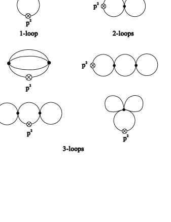
Figure 1: The one-dimensional Feynman graphs up to three-loop order which contribute to the calculation of the bulk pressure in equation (34). The operator insertion for $\left(\psi^{\prime}\right)^{2}$ is shown and corresponds to the insertion of the factor $p^{2}~{}$ in the appropriate loop integral.

A standard Feynman graph expansion of closed loops for $\langle\left(\psi^{\prime}\right)^{2}\rangle$ can be obtained and hence the pressure can be calculated from equation (34). Standard dimensional analysis shows that the series obtained is in inverse powers of $m$ and that a diagram with $l$ loops behaves as $m^{2-l}~{}$. To three-loop order we evaluate the diagrams shown in figure 1 and find

$$P_{bulk}~{}=~{}\rho~{}+~{}{e^{2}\over 2}\left(-{m\over 2}~{}+~{}{1\over 16}~{}+~{}{3\over 512m}\right)~{}\ldots~{}.$$ (37)

In order to express $P_{bulk}$ as a function of the density, $\rho$, we use equation (33) and calculate $\rho$ in the loop expansion. As before, the diagrams with $l$ loops behave as $m^{2-l}~{}$. If $P$ is calculated to $l$-loop order, then $\rho$ is needed to $(l-1)$-loop order. To two-loop order we find

$$\rho~{}=~{}e^{2}m^{2}\left(1-{1\over 4m}\right)~{}.$$ (38)

Note that, alternatively,

$$\rho~{}=~{}{m\over 2}\,{\partial P_{bulk}\over\partial m}~{},$$ (39)

and if we define $t=\log(m)$ and write $~{}P_{bulk}=\rho+P_{e}~{}$ then we have

$${d\rho\over dt}-2\rho~{}=~{}-{dP_{e}\over dt}~{},$$ (40)

which has solution

$${\rho\over m^{2}}~{}=~{}\int_{m}^{\infty}\,{1\over m^{2}}\>{dP_{e}\over dm}\>dm~{}+~{}1~{},$$ (41)

where we have used the boundary condition that $\rho/m^{2}\rightarrow 1$ as $m\rightarrow\infty~{}$.

Then $P(m)$ can be re-expressed as a series in $\sqrt{\rho/e^{2}}~{}$:

$$P_{bulk}~{}=~{}\rho~{}-~{}{1\over 4}\sqrt{\rho e^{2}}~{}+~{}{1\over 1024}\sqrt{e^{6}\over\rho}~{}+~{}\ldots~{}.$$ (42)

This agrees with Lenard [2] and it is relatively easy to evaluate the loop expansion to higher orders to improve on Lenard’s result. The second term is the familiar Debye-Hückel contribution and it should also be noted that the two-loop contribution is zero.

3.3 The bulk pressure

In figure 2 we show the computed value for $P_{bulk}$ compared with the predictions of the previous two sections. For convenience $P_{bulk}$ has been scaled by a factor of $e^{2}/2$. As can be seen the curves from equations (24 and (37) fit very well except in the region $0.7<a<1.1~{}$ where even so the discrepancy is not very large.

4 Thin Films: Finite size Effects and Surface Charge Regulation

When the intersurface distance of the film becomes small in the sense that ${1\over 2}e^{2}L$ is no longer large, then we may not apply the thermodynamic result (23).

However if ${1\over 2}ae^{2}L$ and ${1\over 2}e^{2}L$ are both small, which is certainly the case for extremely small $L$, then one may expand the operator $\exp(LH)$ in powers of $LH$. To second order in $LH$ one obtains

$$Z=1+2\mu L\lambda+{L^{2}\over 2}(2\mu^{2}(\lambda^{2}+1)-\mu\lambda e^{2})+O(L^{3})$$ (43)

thus yielding $F\approx-2\mu L\lambda$ and $P_{d}=2\mu\lambda+\theta_{\infty}$. Hence one has the limiting value of the disjoining pressure is negative if the value of $\lambda$ is sufficiently small. However, one has the bound that $\gamma_{0}(a)<a$ and hence $\theta_{\infty}>-2\mu$ thus

$$\lim_{L\to 0}P_{d}>2\mu\lambda-2\mu.$$ (44)

Hence the film certainly has a positive disjoining pressure at small differences if $\lambda>1$. The stability of the film at small separations is determined by

$$\lim_{L\to 0}{\partial P_{d}\over\partial L}=2\mu^{2}(1-\lambda^{2})-\mu\lambda e^{2}.$$ (45)

If this term is positive then the film collapses to the point thickness $L=0$. For this to happen one must have

$$\lambda<1,$$ (46)

and

$$\mu>{\lambda e^{2}\over 2(1-\lambda^{2})}.$$ (47)

The value of the surface charge $\sigma$ is given by

$$\sigma=-\lambda e\langle\exp(-i\phi(0))\rangle=-eL\lambda\mu~{}.$$ (48)

Hence over short distances the surface charge decays linearly as the two surfaces are brought together.

5 Intermediate Regime

In the regime between very thick and very thin films we shall resort to a numerical analysis of the problem. There are two methods of interest which we detail in the following sections. For convenience of notation we shall work in units where $L$ is scaled by $e^{2}/2$. That is, a factor of $e^{2}/2$ is absorbed into all length variables.

5.1 The Mathieu function method

The disjoining pressure and other properties of the film can be calculated using the even and odd Mathieu functions that are the eigenfunctions of $H^{*}$ defined in equation (22). The kernel ${\cal K}(L,a)$ defined in equation (30) can be computed as an expansion on the Mathieu function by resolution of the identity on the basis of these states. In this way the disjoining pressure may be in general be written as

$$P_{d}(L)=-{e^{2}\over 2}{\sum_{n=1}^{\infty}\;(\gamma_{0}(a)-\gamma_{n}(a))\;c_{n}^{2}\;\exp(\gamma_{n}(a)L)\over\sum_{n=0}^{\infty}\;c_{n}^{2}\;\exp(\gamma_{n}(a)L)},$$ (49)

where

$$c_{n}=\int_{0}^{2\pi}d\phi\,\chi_{n}(\phi)\exp(\lambda\exp(-i\phi)).$$ (50)

If the eigenvalues of $H$ are arranged in descending order i.e. $\gamma_{0}>\gamma_{1}>\gamma_{2}...$, the corresponding eigenfunctions are even about $\pi$ for $n$ even and odd about $\pi$ for $n$ odd. Hence $c_{n}$ is purely real for $n$ even and purely imaginary for $n$ odd. If $\lambda=0$ then $c_{n}=0$ for $n$ odd and hence $P_{d}$ is always negative, hence the force between the two interfaces is always attractive. One sees from the above expression that it is the even wave functions which are attractive and the odd wave functions which are repulsive (as the demoninator on the RHS of (49) is $Z$ and hence positive). At long distances

$$P_{d}\sim{e^{2}\over 2}{c_{1}^{2}\over c_{0}^{2}}\;(\gamma_{0}-\gamma_{1})\;\exp(L(\gamma_{1}-\gamma_{0}))~{}>~{}0$$ (51)

Hence for a non-zero $\lambda$ the long distance disjoining pressure is always positive since $c_{1}^{2}<0~{}$. It is clear however that the disjoining pressure may become negative at smaller values of $L$.

The anion and cation number densities as a function of $x$, the distance through the film, may also be calculated. Denoting these densities respectively by $\rho_{+}$ and $\rho_{-}$ we find

$$\rho_{\pm}~{}=~{}\mu\langle f^{*}|\chi_{n}\rangle\,\exp(-\gamma_{n}x)\,\langle\chi_{n}|e^{\pm i\phi}|\chi_{m}\rangle\,\exp(-\gamma_{m}(L-x))\,\langle\chi_{m}|f\rangle~{},$$ (52)

where

$$\langle\psi|\chi\rangle~{}=~{}\int d\phi\,\psi^{*}(\phi)\chi(\phi)~{}.$$ (53)

We are able to construct both the even and the odd Mathieu functions and their eigenvalues for any value of $a$ using Given’s method for diagonalizing a tri-diagonal matrix. The eigenfunctions of $H^{*}$ are found on a discretization of the interval $[0,2\pi]$ and the appropriate matrix elements in equations (49, 52) can be calculated numerically.

5.2 Fourier method

It turns out that there is a more direct method to calculate the disjoining pressure which exploits the periodicity inherent in the system. This method is especially effective for low temperature (small $e$). It does, however, become much more complicated when other observables such as the density profiles are being calculated. Expanding $K$ in terms of its Fourier modes, i.e. writing

$$K(\phi|x)=\exp(ax)\sum_{n=-\infty}^{\infty}b_{n}(x)\exp(in\phi),$$ (54)

one has that

$$b_{n}(0) = {\lambda^{-n}\over(-n)!}\hbox{ for }n\leq 0$$ (55)

$$= 0\ \ \ \ \ \ \hbox{ for }n>0$$

and the $b_{n}$ evolve via the equation

$${db_{n}\over dx}=-n^{2}b_{n}+a(b_{n+1}+b_{n-1}-2b_{n})/2.$$ (56)

Finally the partition function is given by

$$Z=\exp(aL)\sum_{n=0}^{\infty}{\lambda^{n}\over(n)!}b_{n}.$$ (57)

In this regime we shall also be interested in the mean value of the surface charge $\sigma$. Including a source term in the original formulation of the problem it is a simple matter to show that

$$\sigma=\lambda e\langle\exp(-i\phi)\rangle={\lambda e\over Z}{{1\over 2\pi}}\int_{0}^{2\pi}d\phi_{0}\exp(-i\phi_{0})f(\phi_{0})\exp(LH)f(\phi_{0}).$$ (58)

In terms of the Fourier expansion this becomes

$$\sigma={1\over Z}\exp(aL)\sum_{n=0}^{\infty}{\lambda^{n}\over(n)!}b_{-n+1}$$ (59)

The disjoining pressure may be computed similarly.

In what follows we shall consider three cases which are paradigms for the different regimes of high, intermediate and low temperature. Since we have set $kT=1$, high $T$ corresponds to a small charge parameter, $e$ and vice-versa. Apart from an overall dimension-carrying factor the results depend on $e$ and $\mu$ through the combination $a=4\mu kT/e^{2}$, and in what follows we choose $\mu=1$ and hence in our units $a=1/e^{2}~{}$. The three regimes of temperature are characterized by the three values of charge: $e=0.1,1,4~{}$.

5.3 $e=0.1,~{}a=400$

From equation (37) the bulk pressure is $P=1.926$. The major correction to the free particle pressure, $P_{free}=2$, is the Debye-Hückel term and the two and three-loop contributions are a correction of only $\Delta P=0.003~{}$. In figures 3 and 4 we show the pressure $P$ versus film thickness $L~{}$ for various values of $\lambda$ in the range $0.9$ to $1.2~{}$. Also plotted is the prediction for the bulk pressure to which all curves should be asymptotic. As can be seen there is a collapse in all cases shown for $\lambda$. The details of the collapse differ, however, as $\lambda$ increases. For the lower values of $\lambda$ the collapse is to a film of zero thickness which would, of course, be dominated by the detailed structure of the surface physics which we have subsumed in to a layer of zero thickness. Two maxima are clearly visible for $\lambda=0.93,0.95$. The one at larger $L$ is the location of the ordinary collapse point. The maximum at smaller $L$ and the consequent multiple-valuedness of the curve in $L$ versus $P$ in this region implies a hysteresis phenomenon as $P$ is cycled for very thin films. This kind of effect is reminiscent of a first-order transition which predicts that for a 3D film there will be domains of different thicknesses which will grow or contract like 2D bubbles. Of course, it remains to be seen whether intuition from 1D survives for the realistic 3D case. The typical length scale is $O(e^{2}/2)\sim 5\,10^{-3}$, which is very small compared with the values of $L$ plotted in figures 3 and 4.

For the larger values of $\lambda$ plotted the curves the collapse is to a thinner film but not to one of zero thickness. as $\lambda$ increases the maximum at small $L$ eventually disappears and for much larger $\lambda$ the collapse phenomenon itself disappears.

In figure 5 we shown the surface charge $\sigma$ defined in equation (58) as a function of $L$. There is no feature which hints at the presence of the collapse phenomenon appearing in the associated pressure curves, but in all cases $\sigma$ decreases with $L$. For small $L$ the behavior agrees well with the prediction of equation (48).

The anion and cation densities have been computed as a function of $x$ for various values of $L$ using equation (52). For $e=0.1$ the variation with $x$ is mild and shows no features of note. We show the midplane values for each species as a function of $L$ and for various values of $\lambda$ in figure 6.

It is interesting to note that both methods described in subsections 5.1 and 5.2 were used to calculate the disjoining pressure. However, while 10 fourier modes were amply sufficient, the number of Mathieu modes needed was 40. In particular this large number of modes was found necessary to reproduce the secondary collapse maxima shown in figure 3.

5.4 $e=1.0,~{}a=4$

As in the previous section the pressure $P$ versus $L$ is plotted in figure 7 for values of $\lambda$ in $0.3\leq\lambda\leq 0.8$ which span a region of collapse. In this case there is just one point of collapse to a film of zero thickness (in our approximation) and which disappears for $\lambda$ between $0.7$ and $0.8$. From equation (37) the bulk pressure is predicted to be $P_{bulk}=1.3262$. From the exact calculation we find $P_{bulk}=1.32584$ which is in good agreement with the prediction. To guide the eye the computed asymptotic value is shown in figure 7. These pressure curves are well reproduced by the Mathieu function method with as few as 8 modes. Unlike the case in the previous section $a=4$ is sufficiently small that the physics is dominated by the lowest-lying Mathieu eigenfunctions. This is mainly due to the fact that $\lambda$ is smaller and so the overlap $\langle\chi_{n}|f\rangle$ falls off more sharply with $n$. This in turn means that the pressure peak occurs for larger $L$ than in the $a=400$ case. However, the large-$a$ result for the bulk pressure, equation (37, 42), still holds very well in this region which means that the Debye-Hückel approximation is good.

The surface charge $\sigma$ is plotted in figure 8 and, as in the previous case, there are no features associated with the pressure maxima of figure 7.

The anion and cation number densities as a function of distance, $x$, through the film are shown in figure 9 for $\lambda=0.5~{}$. These quantities were calculated using equation (52). The anion (cation) curves are the higher (lower) set in this figure. There are no unusual features and the curves for the other values of $\lambda$ in $0.3\rightarrow 0.8$ are of similar form.

5.5 $e=4.0,~{}a=0.25$

The pressure $P$ is plotted versus $L$ for $\lambda=0.12,0.121,0.122,0.123$ in figure 10. The collapse region is again evident but it should be noted that it occurs only for a very narrow range of $\lambda$ values. Of course, $\lambda$ is a parameter that is determined by other variables and is not fixed externally. The bulk pressure is no longer given by the large-$a$ expression (equations (37, 42) but is well fitted by the small-$a$ result (equations (24), 27). The prediction is $P_{bulk}=0.243529$ and the computed value is $P_{bulk}=0.243531$. This value is shown for reference in figure 10.

The curves for the surface charge, $\sigma$, are similar to those of previous sections and are not reproduced here. The small $L$ behavior is again consistent with equation (48).

The anion and cation number densities (equation (52) are plotted for $\lambda=.123$ and $L=0.1,0.51.1$ in figure 11. It is interesting to note that for both species the density falls sharply at the film surface and the anion density reaches a peak for the thicker films which is located only a short distance into the film. The position and shape of this peak is independent of thickness $L$ and seems to be a universal feature of the low temperature case. Only the lowest 4 Mathieu modes make an appreciable contribution since the effective charge is large and from equation (52) this causes a strong exponential suppression on all but the lowest modes (note that in equation (52) a factor of $e^{2}/2$ is absorbed into all lengths). Also, the values of $\lambda$ in the collapse region decrease as $e$ increases and so the surface function $f(\phi)$ (equation (14)) oscillates less fast and only has appreciable overlap with the lowest modes. For these reasons the species number densities are dominated by the contributions from the lowest modes and so show more structure at low temperature than at high temperature. This is to be expected since the electrostatic energy dominates the thermal energy. We have observed similar maxima in the density profiles for other values of $e$ if $\lambda$ is sufficiently small. This is due again to the dominance of only a very few low-lying Mathieu modes.

6 Comparison with Poisson-Boltzmann Theory

The Poisson-Boltzmann (PB) theory for our system may either be derived directly by standard thermodynamic techniques [8, 9], or as the mean field theory for the field theory (1). The theory has been used in a wide context in soft condensed matter physics and in particular to analyze the behavior of soap films in [11, 12], and also in the context of colloidal stability [9]. In general it is fair to say that it has been reasonably successful in predicting the physics of systems where interplane distances are reasonably large and for monovalent ionic species [15].

The resulting equations are (again scaling so that $\beta=1$)

$${d^{2}\phi\over dx^{2}}=2\mu e\sinh(e\phi)+\lambda e(\delta(x)\exp(e\phi(0))+\delta(x-L))\exp(e\phi(L))),$$ (60)

where here $\phi$ is the mean field electrostatic field. Assuming symmetry about the point $L/2$ (however see the comments in the conclusion) and using the condition of electroneutrality (which is a mean field assumption), the boundary conditions are

$${d\phi\over dx}|_{0,L}={d\phi\over dx}|_{L\over 2}=0$$ (61)

Interestingly $\phi$ appears as a purely imaginary saddle point of the theory (1). In the region $[0^{+},L^{-}]$ the above equation reduces to

$${d^{2}\phi\over dx^{2}}=2\mu e\sinh(e\phi),$$ (62)

with the boundary conditions

$${d\phi\over dx}|_{L\over 2}=0$$ (63)

and

$${d\phi\over dx}|_{0}=-\lambda e\exp(e\phi(0))=\sigma,$$ (64)

where $\sigma$ is the surface charge. It easy to show that the mean field free energy over the bulk is [8]

$$F_{MF}=\int^{L}_{0}(\phi^{\prime})^{2}\,dx~{}-~{}\left(2\lambda\exp(\beta e\phi(0))+2\mu L(\cosh(e\phi(L/2))-1)\right)~{}.$$ (65)

Then we find

$$P_{d}={2\mu}(\cosh(e\phi_{m})-1)~{},$$ (66)

where $\phi_{m}=\phi(L/2)$ is the midplane potential. One immediately sees that in the case $\lambda=0$ then $\phi=0$ is a solution and the film is always marginally stable in the sense that $P_{d}=0$. In general any non-zero $\lambda$ gives a non-zero value of $\phi_{m}$ and hence the film is always stable for non-zero $\lambda$. This is clearly at variance with the exact results derived here. Moreover, the mean field bulk pressure is $P_{bulk}=2\mu$ which is only applicable to the limit $e\rightarrow 0$ or, equivalently, $a\rightarrow\infty$.

In general one must resort to a numerical solution of the above mean field equations. However in the case where $L$ is small such that $\phi$ varies only slightly we may use the approximation,

$$\phi=\phi_{m}+C(x-{L\over 2})^{2}.$$ (67)

Substituting this into equation (62) yields $C=\mu e\sinh(\phi_{m})$. Using this in the boundary condition (64) then yields

$$\mu L\sinh(e\phi_{m})=-\lambda\exp(e\phi_{m})+O(L^{2}).$$ (68)

Solving this yields

$$\phi_{m}=-{1\over 2e}\log({2\lambda\over\mu L}+1).$$ (69)

Hence in this limit

$$P_{d}(L)\sim\sqrt{2\lambda\mu\over L}$$ (70)

and

$$\sigma\sim-e\sqrt{L\mu\lambda\over 2}.$$ (71)

One sees that while the surface charge $\sigma$ does decay to zero it does so as $L^{1\over 2}$ in comparison with the exact result (48). In addition the disjoining pressure (70) actually diverges rather than tending to a constant.

For infinitely thick films one may use the condition that $\phi_{m}\to 0$ in order to calculate the surface potential. In this case the surface potential is given by the equation

$$\cosh(e\phi(0))-{1\over 4\mu}\lambda^{2}e^{2}\exp(e\phi(0))=1,$$ (72)

from this we find that the physical solution is

$$\phi(0)=-{1\over e}\log(1+\lambda e/\sqrt{2\mu})$$ (73)

giving a surface charge

$$\sigma={-\lambda e\over 1+\lambda e/\sqrt{2\mu}}.$$ (74)

At intermediate distances one has to numerically solve the PB equations. For the cases discussed in section 5 there is no agreement at all between the numerical solution to the PB equation and the exact result. This is to be expected since there is no collapse predicted by the PB equation. However, there is no agreement even on the rising part of the pressure curve at $L$ much greater than that at the pressure maximum. Also, the values of $P_{bulk}$ are not close to the mean-field prediction of $P^{MF}_{bulk}=2.0$ although for $e=0.1$ this value is approached. Nevertheless, in this latter case there is still a large disagreement between the exact and mean-field curves. Indeed, we have investigated very small values of $e$ for a large range of $\lambda$ values but have not found any reliable agreement between the exact theory and the PB equation. The PB equation may be applicable for even smaller values of $e$ than we have investigated. Indeed, a naive analysis of the applicability of the saddle point method for the theory (1) suggests that $a$ should be large, i.e., either $\mu\gg 1$ or $e^{2}\ll 1$, thus giving either $\mu$ or $1/e^{2}$ as the large parameter justifying the saddle point analysis. However, in the cases we have analyzed here, mean-field theory and the PB equation are of very little value in the analysis of the one-dimensional Coulomb gas.

7 Conclusions

In conclusion we have derived an exact solution for the one dimensional Coulomb gas with boundary effects. Surprisingly the mere presence of a boundary, without any surface adhesion term, leads to a reduction of the density near the boundary with respect to the bulk. This effect means that the disjoining pressure of the system is negative and the resulting film will tend to collapse. When $\lambda>0$ we have shown that at sufficiently large distances the disjoining pressure must be positive, and hence a stable common film regime exists. However, if the value of $\lambda$ is not too large a collapse phenomena may occur where the disjoining pressure decreases as the surfaces come together. The disjoining pressure may even become negative signalling the onset of strong attractive forces in the system; this may well be the one dimensional version of the collapse to a NBF seen in experimental systems. We have also seen the possibility of secondary collapses in the parameter ranges we have studied; it would be interesting if one could find an experimental system exhibiting a secondary collapse. In principle multiple collapses are possible, but we have yet to see more than two.

Poisson-Boltzmann theory predicts a stable film for any non-zero value of $\lambda$ and in addition the calculated mean field disjoining pressure is larger that that of the exact calculation. Taking into account the full theory and all its correlations does indeed introduce an attractive interaction over and above the mean field result, in accordance with the calculations made in three dimensional systems using techniques beyond mean field theory [5, 6, 14]. We would like to comment here that in our solution of the mean field equations we have, as is done throughout the literature, always assumed that the mean field solution is symmetric about the midplane of the film. In physical terms this seems quite plausible for thick films where the two planes do not interact and hence there can be no breaking of spatial symmetry. The variant of mean field theory used in [12, 13] uses this symmetric solution and the theory describes extremely well both surface tension data for SDS bulk solutions and the disjoining pressure isotherms up to the point where the collapse occurs. One may show [16] in the field theoretic sense that the mean field solutions we have found here and in [12, 13] are indeed stable local minima of the free energy and hence they at least describe a metastable state. The fact that the mean field solutions work so well in this context up to the collapse point suggest that another mean field solution with a broken spatial symmetry and possibly with a complex part may appear with a lower free energy than that of the symmetric real solution. This would also be consistent with the experimental indications (and indeed conclusions that may be drawn from our exact solutions in 1 D) that the transition to a Newton Black Film is of first order. Work on this problem is currently under progress [16].

Acknowledgments

The authors would like to thank J.J. Benattar, R. Bidaux, I.T. Drummond and H. Orland for useful discussions.

Figure 2: The bulk pressure $P_{bulk}$, scaled by $e^{2}/2$ versus $a=4\mu/e^{2}~{}$. The solid line is the exact computed curve and the dashed and long-dashed curves are the predictions of equations (24) and (37), respectively. The predictions fit very well except in the region $0.7<a<1.1~{}$.

Figure 3: The pressure $P$ versus film thickness $L$ for $kT=1.0$, $e=0.1$ and $\mu=1.0$. for $0<L\leq 10.0$. The different curves are for $\lambda=0.9,0.93,0.95,0.97,1.02,1.2~{}$ which respectively correspond to the curves from lowest to highest pressure at any given $L$. The phenomenon of primary and, in some cases, secondary collapse are clearly visible.

Figure 4: The curves shown in figure 3 extending to larger $L$ to highlight the region of primary collapse. As in figure 3 the higher the value of $\lambda$ the higher the pressure at given $L$.

Figure 5: The surface charge $\sigma$ defined by equation (48) versus film thickness $L$ for $kT=1.0$, $e=0.1$ and $\mu=1.0$. The different curves are for $\lambda=0.9,0.93,0.95,0.97,1.02,1.2~{}$ corresponding to the curves from lowest to highest $\sigma$. There is no feature which hints at the presence of the collapse phenomenon appearing in the pressure curves shown in figures 3 and 4.

Figure 6: The midplane anion (upper curves) and cation (lower curves) densities as a function of film thickness $L$, for $e=0.1,\mu=1$, $\lambda=0.9$ (solid) and $1.2~{}$ (dashed).

Figure 7: The pressure $P$ versus film thickness $L$ for $kT=1.0$, $e=1.0$ and $\mu=1.0$. The different curves are for $\lambda=0.3,0.4,0.5,0.6,0.7,0.8~{}$ which respectively correspond to the curves from lowest to highest pressure at any given $L$. The collapse phenomenon occurs for the smaller $\lambda$ values and disappears between $\lambda=0.7$ and $\lambda=0.8$.

Figure 8: The surface charge $\sigma$ defined by equation (48) versus film thickness $L$ for $kT=1.0$, $e=0.1$ and $\mu=1.0$. The different curves are for $\lambda=0.9,0.93,0.95,0.97,1.02,1.2~{}$ corresponding to the curves from lowest to highest $\sigma$. There is no feature which hints at the presence of the collapse phenomenon appearing in the pressure curves shown in figures 3 and 4.

Figure 9: The anion (solid curves) and cation (dashed curves) densities as a function of distance $x$ through the film for $e=1.0,\mu=1$, $\lambda=0.95$ and for various film thickness $L$.

Figure 10: The pressure $P$ versus film thickness $L$ for $kT=1.0$, $e=4.0$ and $\mu=1.0$. The different curves are for $\lambda=0.12,0.121,0.122,0.123~{}$ which respectively correspond to the curves from lowest to highest pressure at any given $L$. The collapse phenomenon occurs for the smaller $\lambda$ values and disappears between $\lambda=0.122$ and $\lambda=0.123$.

Figure 11: The anion (solid curves) and cation (dashed curves) densities as a function of distance $x$ through the film for $e=4.0,\mu=1$, $\lambda=0.123$ and for film thicknesses $L=0.1,0.5,1.1$.

References

- [1] S. Edwards and A. Lenard, J. Math. Phys. 3, 778, (1962)
- [2] A. Lenard, J. Math. Phys. 2, 682, (1961)
- [3] S. Prager, Advances in Chemical Physics IV, 201, Wiley (Interscience), New York (1962).
- [4] E.H. Lieb and D.C. Mattis, Mathematical Physics in One Dimension, Perspectives in Physics, (Academic Press), New York and London, (1966).
- [5] O. Spalla and L. Belloni, J. Chem. Phys. 95, 10 (1991)
- [6] O. Spalla and L. Belloni, Phys. Rev. Lett. 74, 13 (1995)
- [7] F. Cornu and B. Jancovici, J. Chem. Phys. 90, 4, 2444, (1989)
- [8] J. Israelachvili, Intermolecular and Surface Forces, (Academic Press), (1992)
- [9] I.B. Ivanov (editor), Thin Liquid Films (Fundamentals and Applications), Surfactant Science Series (Marcel Dekker, Inc.), (1988); J. Lykelma, Fundamentals of Interface and Colloid Science (Volume 1: Fundamentals), (Academic Press), (1991).
- [10] J.T. Davies, Proc. Roy. Soc. A, 245, 417 (1958)
- [11] D. Exerowa, T. Kolarov and Khr. Khristov, Colloids and Surfaces, 22, 171 (1987)
- [12] D.S. Dean and D. Sentenac to appear Europhys. Lett.
- [13] D.S. Dean and D. Sentenac submitted J. Colloid Interface Sci.
- [14] R. Podgornik, J. Chem. Phys. 91, 9, (1989)
- [15] D. Andelman, J. Phys. Chem. 100, 32, 13732, (1196)
- [16] D.S. Dean, R.R. Horgan and D. Sentenac work in progress
- [17] Abramowitz and Stegun, ”Handbook of Mathematical Functions”, Dover Publications, 1964.
- [18] R.D. Coalson and A. Duncan, J. Chem. Phys. 97, 5653, (1992)
- [19] N. Ben-Tai and R.D. Coalson, J. Chem. Phys. 101, 5148, (1994)
for is shown and
corresponds to the insertion of the factor in the appropriate loop integral.
for is shown and
corresponds to the insertion of the factor in the appropriate loop integral.