[

Modification of the Landau-Lifshitz Equation in the Presence of a Spin-Polarized Current in CMR and GMR Materials.

Abstract

We derive a continuum equation for the magnetization of a conducting ferromagnet in the presence of a spin-polarized current. Current effects enter in the form of a topological term in the Landau-Lifshitz equation . In the stationary situation the problem maps onto the motion of a classical charged particle in the field of a magnetic monopole. The spatial dependence of the magnetization is calculated for a one-dimensional geometry and suggestions for experimental observation are made. We also consider time-dependent solutions and predict a spin-wave instability for large currents.

]

Phenomena associated with spin-polarized currents in layered materials and in Mn-oxides have attracted high interest recently. Efforts are strongly concentrated on theoretical and experimental investigation of large magnetoresistance, which is of great value for future applications. Examples of the effect are GMR in layered materials (see review [1]), spin valve effect for a particular case of a three-layer sandwich and CMR in the manganese oxides (see review [2]).

The dependence of resistivity on magnetic field is explained conceptually in two steps: first the magnetic field changes the magnetic configuration of the material and that in turn influences the current. Of course, as for any interaction there must be a back-action of the current on the magnetic structure. The existence of such back-action was explored in [3, 4]. Several current-controlled micro-devices utilizing this principle were proposed [3]. In both papers layered structures with magnetization being constant throughout the magnetic layers were considered. In the present paper we derive the equations for a continuously changing magnetization in the presence of a spin-polarized current. This equation takes the form of a Landau-Lifshitz equation with an additional topological term, and admits a useful analogy with a mechanical system. We discuss several solutions in one-dimensional geometries. Our equations also can be viewed as a continuum generalization of [3, 4] for layer thickness going to zero.

Consider a current propagating through a conducting ferromagnet. Conducting electrons are viewed as free electrons interacting only with local magnetization $\bf M$. The motion of each individual electron is governed by the Schroedinger equation with a term $J_{H}\mbox{\boldmath$\sigma$}{\bf M}$, where $J_{H}$ is the value of the Hund’s rule coupling or in general of the local exchange. Since spin-up electrons have lower energy a nonzero average spin of conducting electrons $(1/2)\langle\mbox{\boldmath$\sigma$}\rangle$ develops. An angular momentum density $(\hbar/2)\langle\mbox{\boldmath$\sigma$}\rangle$ is then carried with the electron current so we have a flux of angular momentum. This leads to a non-zero average torque acting on the magnetization which can deflect it from the original direction (see figure 1).

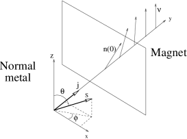
FIG. 1.: Experimental setting: spin-polarized current enters a half-infinite magnet from the left. Originally the magnetization is aligned along the easy-axis $\nu\|z$. However if the incoming electrons are spin-polarized in a different direction, their interaction with the magnetization leads to a deflection of the magnetization.

Propagation of a current in a ferromagnet should be described by a system of two equations: one for the motion of conducting electrons and another for the magnetization. We derive here the second equation in the limit of small space-time gradients and present several solutions. The case of very large $J_{H}\to\infty$ is considered, meaning a complete polarization of electron spins in the ferromagnet. This case can be often realized in experiment. In the layered structures magnetic layers can be made of a material with large band splitting, like Heusler alloys, in which the spin opposite to magnetization direction can not propagate. In the CMR materials large Hund’s rule coupling is well known [2] and constitutes the basis for a double-exchange mechanism governing their magnetic ordering.

Schroedinger Equation: the conducting electrons are considered noninteracting with an $\varepsilon=p^{2}/2m$ energy spectrum:

$$i\hbar\frac{\partial\psi_{\alpha}}{\partial t}=-\frac{\hbar^{2}}{2m}\Delta\psi_{\alpha}+J_{H}{\bf M}({\bf r},t)\mbox{\boldmath$\sigma$}_{\alpha\beta}\psi_{\beta}$$ (1)

We diagonalize the matrix ${\bf~{}M(r},t)\mbox{\boldmath$\sigma$}_{\alpha\beta}$ with a local spin rotation $\phi_{\alpha}={U}_{\alpha\beta}({\bf~{}r},t)\psi_{\beta}$. The spinor $\phi$ describes the electron in the coordinate system with $z$-axis being parallel to the local magnetization. Retaining only the first order terms in gradients and using $\phi_{-}\to 0$ for $J_{H}\to\infty$ we reduce (1) from a system of two equations to one equation for $\phi_{+}\equiv\phi$ spin amplitude:

$$i\hbar\frac{\partial\phi}{\partial t}=-\frac{\hbar^{2}}{2m}\Delta\phi+J_{H}M\phi-\frac{\hbar^{2}}{2m}(U_{+\beta}\nabla_{i}U_{\beta+})\nabla_{i}\phi$$ (2)

The last term in (2) can be transformed (${\bf M}=M{\bf n}$ ):

$$i\hbar\frac{\partial\phi}{\partial t}=-\frac{\hbar^{2}}{2m}\Delta\phi+J_{H}M\phi-\frac{i\hbar^{2}}{4m}A_{\rm mon}^{k}({\bf n})\nabla_{i}n^{k}\nabla_{i}\phi$$ (3)

where ${\bf A}^{\rm mon}({\bf n})$ is a function satisfying the following equations:

$$\epsilon_{\alpha\beta\gamma}\frac{\partial A_{\beta}^{\rm mon}}{\partial n_{\gamma}}=2n_{\alpha}\ ,\;\;\frac{\partial A_{\alpha}^{\rm mon}}{\partial n_{\beta}}=\epsilon_{\alpha\beta\gamma}n_{\gamma}$$

If we view $n^{2}({\bf r},t)=1$ as a sphere, ${\bf A}^{\rm mon}$ has the simple interpretation of the vector potential due to a magnetic monopole located at the center of the sphere. The monopole term is known to appear from $U_{+\beta}\nabla_{i}U_{\beta+}$ in the theory of Berry phase and is used by other CMR theories in different forms (see [5]). Equation (3) has a form of a Schroedinger equation in a magnetic field expanded up to the linear term in ${\bf A}^{\rm eff}$, with vector potential $A_{i}^{\rm eff}=(i\hbar^{2}/4m)A_{\rm mon}^{k}\nabla_{i}n^{k}$. It describes the motion of the conducting electrons in the given field ${\bf n}({\bf r},t)$. Conversely it gives the interaction between the current and the magnetization. The form of equation is the same as for an electromagnetic interaction, and hence we can write by analogy:

$$E_{\rm int}=\frac{1}{c}j_{i}A_{i}^{\rm eff}=-\frac{\hbar}{4}\frac{j_{i}}{e}A_{\rm mon}^{k}({\bf n})\nabla_{i}n^{k}$$ (4)

where ${\bf j}$ is an electric current.

Magnetization motion is described by Landau-Lifshitz equations which are obtained from the energy functional. After adding (4) to the usual energy density of a ferromagnet with uniaxial anisotropy along the axis $\nu$, we obtain:

$$E=\int[J({\bf\nabla M})^{2}-K(\mbox{\boldmath{$\nu$}}{\bf n})^{2}+\frac{1}{c}j_{i}A_{i}^{eff}]dV$$ (5)

with $K>0$ corresponding to easy-axis and $K<0$ to easy-plane magnets. The equations of motion then take the form:

$$\frac{\partial{\bf M}}{\partial t}=\frac{g\mid e\mid}{2mc}[{\bf f}\times{\bf M}]]$$ (6)

$${\bf f}=-\frac{\delta E}{\delta{\bf M}}=J\Delta{\bf M}+\frac{2K}{M^{2}}({\bf\mbox{\boldmath{$\nu$}}M})\mbox{\boldmath{$\nu$}}+\frac{\hbar}{2M}\frac{j_{i}}{e}[\nabla_{i}{\bf n}\times{\bf n}]$$ (7)

where the last term in $\bf f$ is new and describes the effect of the current. The system of (3) and (6,7) constitute a complete set of equations for a magnet with current. Equations (6,7), generalizing the Landau-Lifshitz equation in the presence of a current, are the central result of this work.

Since magnetization corresponds to angular momentum ${\bf L}=\hbar/g\mu_{B}\;{\bf M}$, an equation of the angular momentum flux continuity follows from (7):

$$\frac{\partial L_{k}}{\partial t}+\frac{\partial\Lambda_{ki}}{\partial x_{i}}=\left[\frac{2g\mu_{B}K}{\hbar M^{2}}({\bf\mbox{\boldmath{$\nu$}}n})\mbox{\boldmath{$\nu$}}\times{\bf M}\right]_{k}$$ (8)

$$\Lambda_{ki}=M^{2}J[{\bf n}\times\nabla_{i}{\bf n}]_{k}+\frac{\hbar}{2}(\frac{j_{i}}{e}n_{k})$$ (9)

The flux $\Lambda_{ki}$ consists of two parts: one due to the spatial derivatives of magnetization and another due to the motion of conducting electrons. In our situation the spins of moving electrons are parallel to ${\bf n}$. That is why their contribution is factorized in the form $(\hbar/2)(j_{i}/e)n_{k}$.

Consider the stationary case in an experimental setting shown on figure 1. For the stationary process the r.h.s. of equation (6) vanishes. The current propagates along the ${\hat{\bf y}}$ direction. All spatial derivatives reduce to $\mbox{\boldmath$\nabla$}\rightarrow\nabla_{y}$. For the reasons immediately following we will denote differentiation with a prime to get a resemblance to a time derivative in notation $\nabla_{y}{\bf~{}n}\equiv{\bf n^{\prime}}$. From (7) we get an equation on ${\bf n}({\bf r},t)$:

$${\tilde{J}}[{\bf n}^{\prime\prime}\times{\bf n}]=[(-{\tilde{K}}({\bf\mbox{\boldmath{$\nu$}}n})\mbox{\boldmath{$\nu$}}-Q(\frac{j}{e})[{\bf n^{\prime}}\times{\bf n}])\times{\bf n}]$$ (10)

with new parameters:

$$\tilde{J}=\frac{g\mu_{B}M}{\hbar}J,\;\;\tilde{K}=\frac{2g\mu_{B}}{\hbar M}K,\;\;Q=\frac{g\mu_{B}}{2M}$$

Since $\bf n$ in the stationary case depends on $y$ only, we can interpret $y$ as a fictitious time; together with ${\bf n}^{2}=1$ equation (10) can then be interpreted as the equation of motion for a particle of a mass $\tilde{J}$ confined to the surface of a unit sphere and experiencing two forces:
(a) a force of magnitude $-{\tilde{K}}({\bf\mbox{\boldmath{$\nu$}}n})\mbox{\boldmath{$\nu$}}$ parallel to the anisotropy axis,
(b) a Lorentz force , due to a field ${\bf H}_{\rm mon}=-Q(\frac{j}{e}){\bf n}$ of a magnetic monopole positioned in the center of the sphere.
The vector product ensures that only tangential components of the total force act on the particle. The normal component is compensated by the reaction forces. Such an anology enables one to visualize the soluctions of the original equation (10) as trajectories of a massive particle on the sphere.

The equation of particle motion in the field of a magnetic monopole (10) has two first integrals [7].

$$W=\frac{\tilde{J}{\bf n^{\prime}}^{2}}{2}+\frac{{\tilde{K}}({\bf\mbox{\boldmath{$\nu$}}n})^{2}}{2}={\rm const}$$ (11)

$$D_{\nu}={\tilde{J}}([{\bf n}\times{\bf n^{\prime}}]\nu)+Q(\frac{j}{e})({\bf n\mbox{\boldmath{$\nu$}}})={\rm const}$$ (12)

Together they give a way to solve (10 ) for arbitrary initial conditions. Expressing everything through the Euler angles $\{\phi(y),\theta(y)\}$ (defined on figure 1) of the vector $\bf n$ , we obtain:

$$\phi^{\prime}=\frac{D_{\nu}-Q(j/e)\cos\theta}{\tilde{J}\sin^{2}\theta}$$

$$\theta^{\prime} = \sqrt{\frac{2W-\tilde{K}\cos^{2}\theta}{\tilde{J}}-\frac{(D_{\nu}-Q(j/e)\cos\theta)^{2}}{{\tilde{J}}^{2}\sin^{2}\theta}}$$ (13)

$$\equiv {\cal F}(\theta)$$ (14)

The problem for $\theta$ is solved by the implicit function:

$$y=y(0)+\int_{\theta(0)}^{\theta}\frac{d\theta}{{\cal F}(\theta)}$$ (15)

afterwards $\phi$ can be found from the first equation in (13).

Assume that deep inside the magnet ($y\to\infty$) the magnetization resumes its original direction along the anisotropy axis ${\bf n}\to\mbox{\boldmath{$\nu$}},\;\;{\bf n}^{\prime}\to 0$. From this the values of the first integrals can be found and substituted into (13). Natural length and current scales appear in the calculation:

$$L_{m}=\sqrt{\frac{JM^{2}}{8K}},\;\;\;j_{0}=\frac{e}{\hbar}\sqrt{KJM^{2}}$$ (16)

through which the material parameters $J,K,M$ enter the problem. Their values for different materials are given in the following table:

Material	$L_{m}\;\;[\AA]$	$j_{0}\;\;[{\rm A/cm^{2}}$]	Ref.
CMR: $\rm La_{0.66}Ca_{0.33}MnO_{3}$	$>130$	$<4\cdot 10^{7}$	[8]
Fe	40	$1.1\cdot 10^{8}$	[9]
Heusler Alloy: PtMnSb	$50\sim 100$	$\sim 5\cdot 10^{7}$	[10]

The integral (15) can be then expressed in elementary functions but the formula is long and will be detailed in a later paper. Instead, the results are presented on figure 2. It is seen that magnetization relaxes in a distance $\approx 10L_{m}$ which is about the width of the domain wall in the material.

In the “particle picture” the motion starts at some point $A$ on the trajectory, yet to be determined from the b.c. on the normal metal - magnet interface, and ends on the North pole. The particle has just enough energy to climb the potential hill and come to rest on the top. The particle trajectory is bent by the monopole field. In the absence of the monopole the particle would go along the meridian.

The boundary condition on the metal-magnet interface, $y=0$ is derived from the continuity of the angular momentum flux. Such condition ensures that there is no torque concentrated on the boundary consistent with the assumption of slow spatial changes of the magnetization.

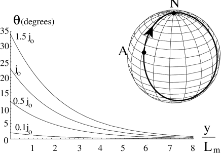
FIG. 2.: Magnetization deflection angle $\theta(y)$. Curves correspond to different values of current, $\theta_{0}=\pi/2,\;p=0.5$. Inset: trajectory of particle on the sphere for $j=j_{0}$. Starting point A corresponds to the conditions of the main graph.

The reflection of the down-spin electron component occurs on the length scale of the electron wavelength. On this distance magnetization is almost constant and solving the one-particle reflection problem we find the jump of the electron flux component in the $\hat{y}$ direction $\Sigma_{i}\equiv\Sigma_{iy}$ to be:

$${\bf\Sigma}_{\rm metal}^{\rm electron}-{\bf\Sigma}_{\rm magnet}^{\rm electron}={\bf\Sigma}-{\bf n}({\bf\Sigma}{\bf n})$$ (17)

where $\bf\Sigma$ is the average injected flux. From (9) the flux inside the magnet is:

$$\Lambda_{i,y}={\bf\Sigma}_{\rm magnet}^{\rm electron}+M^{2}J[{\bf n}_{0}\times{\bf n}^{\prime}_{0}]_{i}$$ (18)

In the metal, only the electron part of the flux is present. Then continuity gives the boundary condition:

$${\bf\Sigma}-({\bf\Sigma n}_{0}){\bf n}_{0}=M^{2}J[{\bf n}_{0}\times{\bf n}^{\prime}_{0}]$$ (19)

Note that it involves both the vector ${\bf n}$ and its derivative on the boundary.

Condition (19) can be transformed into a system of two algebraic equations and an inequality:

$$\frac{1}{2}\left(\frac{pj}{j_{0}}\right)^{2}(1-y^{2})=1-x^{2}$$ (20)

$$p(\cos\theta_{0}-xy)=1-x$$ (21)

$$y^{2}+x^{2}-2yx\cos\theta_{0}\leq\sin^{2}\theta_{0}$$ (22)

where ${\bf\Sigma}=\Sigma~{}{\bf e}$, $\cos\theta_{0}={\bf e\cdot\mbox{\boldmath{$\nu$}}},\;x={\bf\mbox{\boldmath{$\nu$}}\cdot~{}n_{0}},\;y={\bf~{}e~{}\cdot~{}n_{0}}$. The parameter $p=e\Sigma/j,\;\;p\in~{}[0,1/2]$, describes the “degree of polarization” of the incident electrons . The inequality in (20) is a geometrical constraint on $x$ and $y$ arising from their definition.

The trajectory is determined by three parameters: $(j/j_{0},p,\theta_{0})$. We can plot a domain of existence of a solution to (20) in the 3-D space of these parameters. A typical 2-D section of this diagram for constant $\theta_{0}$ is shown in figure 3. A solution is absent in the regions B and C which means that for larger currents and spin-polarizations no smooth stationary solution approaching the easy-axis direction at infinity is available. Either a non-stationary solution or a solution which never approaches $\nu$ will be realized in that region.

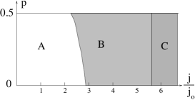
FIG. 3.: A typical 2-D section of the phase diagram plotted for $\theta_{0}=\pi/3$. A: domain of existence of a solution to (20); B: no solution, b.c. at $y=0$ can not be satisfied; C: no solution, b.c. at $y\to\infty$ can not be satisfied and spin wave instability occurs.

Time-dependent solutions of equation (7) can be found in some cases. We again assume the current ${\bf j}$ to be uniform. We rewrite equation (7) through ${\bf n}({\bf r},t)$:

$$\frac{\partial{\bf n}}{\partial t}=[{\bf g}\times{\bf n}]-Q(\frac{j_{i}}{e})\nabla_{i}{\bf n}$$

$${\bf g}={\tilde{J}}\Delta{\bf n}+{\ \tilde{K}}({\bf\mbox{\boldmath{$\nu$}}n})\mbox{\boldmath{$\nu$}}$$ (23)

and suppose $n_{0}({\bf r})$ solves $[{\bf g}\times{\bf n_{0}}]=0$, i.e. represents a static solution in the absence of the current. Then

$$n({\bf r},t)=n_{0}({\bf r}+Q(\frac{{\bf j}}{e})t)=n_{0}({\bf r}+\frac{\omega_{0}L_{m}}{\sqrt{2}}\frac{j}{\ j_{0}}\ t)$$ (24)

where $\omega_{0}=\tilde{K}$, is a solution of (23) for a nonzero current. For instance a moving Bloch wall will be a solution when current is flowing perpendicular to it (provided pinning is absent).

Another particular solution is a spin wave in the presence of a current. We search for a solution (7) in the form of a spin wave: $\{\theta={\rm const},\;\phi={\bf kr}-\omega t\}$. This gives the spectrum:

$$\omega=\tilde{J}k^{2}-Q\frac{{\bf jk}}{e}+\tilde{K}$$ (25)

As we see, the current changes the energy gap of spin waves and shifts the position of the minimum:

$$\omega_{\min}=\tilde{K}-(Q\frac{j}{e})^{2}\frac{\cos^{2}\alpha}{4\tilde{J}}=\omega_{0}(1-\frac{j^{2}}{32j_{0}^{2}}\cos^{2}\alpha)$$

where $\alpha$ is the angle between $j$ and $k$ and $\omega_{0}=\tilde{K}$  is the gap of spin wave in an anisotropic ferromagnet. For large enough current $j>4\sqrt{2}\ j_{0}$ an instability occurs. That is also the condition which leads in the region $C$ on figure 3 to the loss of any trajectory approaching $\nu$ at infinity as the integral (15) becomes undetermined. A spin-wave instability is also predicted in other models of spin-polarized transport [4].

Discussing possible experiments we note that the characteristic current is large, but such densities are in fact common for layered metallic structures and $j\sim j_{0}$ is experimentally possible. In this regime the calculated magnetization profile (figure 2) shows a deviation of $\approx 20^{o}$ on the boundary. Detection of the effect is difficult because the spatial resolution of existing probes exceeds $L_{m}$. For a quantitative measurement of the deflection angle on the boundary, element specific X-ray magnetic circular dichroism (MXCD) [11] could be used. A single layer of different magnetic element can be put on the boundary in the process of the film growth. Such a layer will not much disturb the overall magnetization profile. The MXCD signal of the additional layer could be separated from the Mn signal and thus $\theta(0)$ can be measured. The time-dependent approach developed here can be applied to other experimental geometries, e.g. to find the continuum analogies for the devices proposed in [3].

The authors are greatful to J.Slonczewski for discussion and providing his paper before publication, to L.P.Pryadko, A.J.Millis, V.N.Smolyaninova and K.Pettit for discussions. Research at Stanfrod University was supported by the NSF grant DMR-9522915.

REFERENCES

- [1] W.P.Pratt et al. J.Magn.Magn.Mater., 126, 406 (1993); P.M.Levy,S.Zhang, J.Magn.Magn.Mater. 151, 315 (1995) and papers cited therein
- [2] A.R.Bishop and H.Roder. cond-mat/9703148 (1997), to appear in “Current Opinion in Solid State & Materials Science”, ed.A.K.Cheethawn, H.Inokuchi, J.M.Thomas; Current Chemistry Ltd., London, UK, and papers cited therein
- [3] J.Slonczewski, J.Magn.Magn.Materials, 159, L1 (1996)
- [4] L.Berger, Phys.Rev.B, 54, 9353 (1996)
- [5] A.Auerbach “Interacting Electrons and Quantum Magnetism”, Ch.10, p.103 Springer-Verlag, 1994; Muller-Hartman, E.Daggotto, PRB, 54, R6819 (1996); S.Ishihara, M.Yamanaka, N.Nagaosa, cond-mat/9606160 (1996); B.Doucot, R.Rammal, PRB 41, 9617 (1990)
- [6] L.Berger, Phys.Rev.B , 33, 1572 (1986)
- [7] N.Katayama, Nuovo Cimento, 108B, N.6, 657, 1993; T.Yoshida, Nuovo Cimento, 104B, N.4, 375, 1989 and papers cited therein.
- [8] J.W.Lynn et al., PRL, 76, 4046 (1996); Lofland et al, J. Appl. Phys.81, 5737 (1997)
- [9] D.Jiles, “Introduction to Magnetism and Magnetic Materials”, Ch.7, 134, Chapman and Hall (1990)
- [10] Estimated from and domain wall thickness. R.White, private communication.
- [11] B.Gurney, private communication.