PROTEIN FOLDING AND HETEROPOLYMERS

We present a statistical mechanics approach to the protein folding problem. We first review some of the basic properties of proteins, and introduce some physical models to describe their thermodynamics. These models rely on a random heteropolymeric description of these non random biomolecules. Various kinds of randomness are investigated, and the connection with disordered systems is discussed. We conclude by a brief study of the dynamics of proteins.

Natural proteins have the property of folding into an (almost) unique compact native structure, which is of biological interest $\!{}^{{\bf?},{\bf?}}$. The compactness of this unique native state is largely due to the existence of an optimal amount of hydrophobic amino-acid residues $\!{}^{{\bf?}}$, since these biological objects are usually designed to work in water. The task of predicting the conformation of the three-dimensional structure from the linear primary sequence is often referred to as the protein folding problem. Already at this stage, a rigorous analytical theory appears difficult, since it amounts to study a mesoscopic system (most proteins have between 100 and 500 residues), notwithstanding the solvent’s properties.

This mesoscopic system is of a classical nature; the quantum mechanical valence electrons of the atoms induce interactions between the heavy “nuclei” which can then be treated as classical objects interacting through classical many-body interactions. This observation forms the basis of Molecular Dynamics, Monte Carlo, or Statistical Mechanical models.

To further complicate the matter, both the compactness and the chemical heterogeneity of a given protein tend to slow down dynamical processes: the question of the kinetic control of the folding (as opposed to a thermodynamic control) is therefore periodically asked. This remark suggests that the folding process may have something in common with the physics of glassy systems, where competing interactions (frustration) and/or disorder lead to a very rugged phase space, resulting in slow dynamical processes. In this review, we will assume that the folded state of proteins is thermodynamically stable (the folded state is the state of minimal free energy).

There has been a considerable amount of numerical simulations of proteins, using molecular dynamics or Monte Carlo calculations (for a review see $\!{}^{{\bf?},{\bf?},{\bf?}}$).This promising approach will not be discussed in this review. We will use only analytical approaches throughout. Similarly, models emphasizing the micro-crystalline character of the folded proteins will not be addressed here $\!{}^{{\bf?}}$.

The outline of this review is the following. In the first section, we introduce at an elementary level, some notions of the physics, chemistry and biology of proteins. In the second section, we study (using statistical physics methods) some heteropolymer models which are possibly relevant to the protein folding problem. The phase diagrams of these models bear some qualitative resemblance to the real systems.

In the last section, we tackle the issues of dynamics. In view of the complexity of the problem, we first study the homopolymer case. The heteropolymeric aspect is then studied at a more phenomenological level.

1 Biophysical background

For a review on the biological aspects of protein, the reader is referred to the books $\!{}^{{\bf?},{\bf?},{\bf?}}$.

1.1 Elements of Chemistry

Proteins are biological molecules, present in any living organism. Their biological function include catalysis (enzymes), transport of ions (hemoglobin, chlorophyll, etc…), muscle contraction, … They also are present in virus shells, prions, etc. The biological activity involves a small set of atoms, called the “active site” of the protein, where chemical reactions take place.

Proteins belong to the group of biopolymers, which also comprise nucleic acids (DNA, RNA) and polysaccharides. From a physico-chemical point of view, biopolymers are heteropolymers, made out of different species of monomers. For proteins, the monomers are amino-acids, chosen from twenty different species.

The chemical formula of an amino-acid can be written as:

$$NH_{2}-C_{\alpha}HR-COOH$$ (1)

where $NH_{2}$ is the amine group and $COOH$ is the acidic group (except for proline, which has an imine group). Each amino acid is characterized by its residue $R$ . If the residue is not reduced to a hydrogen atom (such as glycine), the alpha-carbon atom $C_{\alpha}$ is asymmetric. In all known natural proteins, the alpha-carbons have the same chirality (they are all left-handed) and the origin of this asymmetry is not known.

The list of amino acids is:

1. Alanine, Isoleucine, Leucine, Methionine, Phenylalanine, Proline, Tryptophan, Valine.

2. Asparagine, Cysteine, Glutamine, Glycine, Serine, Threonine, Tyrosine.

3. Arginine, Histidine, Lysine.

4. Aspartic acid, Glutamic acid.

For instance, the chemical formula of alanine is:

$$NH_{2}-C_{\alpha}H-CH_{3}-COOH$$ (2)

and that of tryptophan is:

$$NH_{2}-C_{\alpha}H-CH_{2}-C-CH-NH-C_{6}H_{4}-COOH$$ (3)

The smallest residue is glycine, which is just a single $H$ atom, and thus non chiral, and the largest is tryptophan, which contains ten heavy (non hydrogen) atoms.

The above gross classification of amino acids refers to their interactions with water, their natural solvent. Group 1 is made of non polar hydrophobic residues. The three other groups are made of hydrophilic residues. From an electrostatic point of view, group 2 corresponds to polar neutral residues, group 3 corresponds to positively charged residues, and group 4 to negatively charged ones.

The typical size of a protein ranges from approximately 100 amino acids for small proteins to 500 for long immuno-globulins. Due to this rather small size, knots are not present in proteins.

A protein is made by polycondensation of amino acids, which can be schematically written as:

$$NH_{2}-C_{\alpha}HR_{1}-COOH+NH_{2}-C_{\alpha}HR_{2}-COOH\to$$

$$NH_{2}-C_{\alpha}HR_{1}-CONH-C_{\alpha}HR_{2}-COOH+H_{2}O$$ (4)

The repetition of this process produces the protein, a weakly branched polymer, characterized by its chemical sequence $R_{1},R_{2},\cdots,R_{N}$.

The polycondensation produces a “peptide bond” $CONH$, represented in Fig. 1.

Figure 1: Peptide bond. The thick line denotes the backbone.

Due to electronic hybridization, this bond is strongly planar.

One can distinguish two types of degrees of freedom in proteins:

1. Hard degrees of freedom: these are the covalent bonds (linking covalently two atoms along the chain), the valence angles (angle between two covalent bonds) and the peptide bond. These degrees of freedom are very rigid at room temperature, since, as we shall see later, their deformation requires energies much higher than $kT$.

2. Soft degrees of freedom: they are essentially the torsion angles along the backbone chain, and of the side chains. Their energy scale is such that they can easily fluctuate at room temperature.

1.2 The possible states of proteins

Qualitative description of the phases

Although it was long believed that proteins are either denatured or native, it seems now well established that they may in fact exist in at least three different phases. Originally, the phases referred to the biological activity of the protein. In the “native phase”, the protein has its full biological activity, whereas in the “denatured phase”, it does not have any biological activity. It was soon recognized that this change in activity was related to some important structural changes in the protein.

The following classification is widely accepted:

1. Native state
   In this phase, the protein is said to be folded and has its full biological activity; it is compact, globular, and has a unique and well defined three dimensional structure. This implies that in this state, the active site is well defined.

   As we shall discuss later, the uniqueness of the folded state is quite puzzling, given that the number of compact states of a homopolymer of size $N$ is known to behave like $\mu^{N}$ $\!{}^{{\bf?}}$. Even with an extremely conservative value $\mu=2$ and $N=100$, this represents an astronomically large number of compact configurations, and it is quite amazing that proteins always find their ways to the correct folded state. Basically, the conformational entropy of the native state is zero.

   In Fig. 2, we show a graphical representation of the protein crambin, generated from its X-ray data.

   

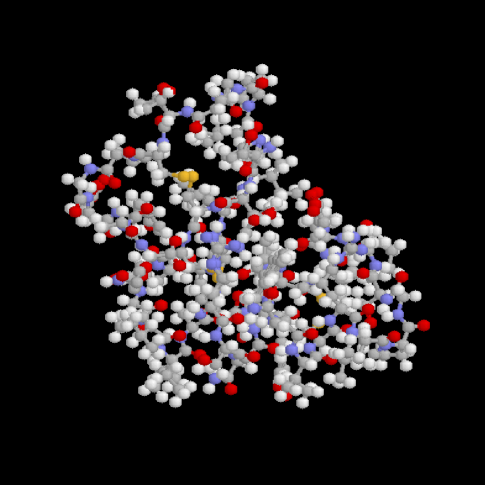
   Figure 2: Computer generated “ball and stick” representation of crambin.

2. Denatured states
   The denatured states are characterized by a lack of biological activity of the protein. Depending on chemical conditions, it seems that there exists at least two denatured phases:

   1. Coil state
      In this state, the denatured protein is in a coil state: it has no definite shape, like a homopolymer in a good solvent. Although in this phase there might be local aggregation phenomena, it is fairly well described as the swollen phase of a homopolymer in a good solvent. It is a state of large conformational entropy.

   2. Molten globule
      At low pH (acidic conditions), some proteins may exist in a compact state, named “molten globule” $\!{}^{{\bf?}}$. This state is compact (the chain is globular); it does not however have a well defined structure and bears strong resemblance to the collapsed phase of a homopolymer in a bad solvent. It is believed that this state is slightly less compact than the native state, and has finite conformational entropy. Anticipating on the next sections, the molten globule seems to have a large content of secondary structure, but not necessarily at the right place (with respect to the native state).

In vitro, the transition between the various phases is controlled by temperature, pH, denaturant agent (such as urea or guanidine).

Time scales

There are two basic time scales in the problem:

1. Microscopic
   The shortest time involved in protein dynamics is related to the vibrational modes of the covalent bonds. The associated time scale is $10^{-15}$s.

2. Macroscopic
   Typical times for the folding of a protein ranges from $10^{-3}$s to $1$s. This is many order of magnitudes larger than the microscopic time, and it is quite puzzling to understand why such a long time is necessary for such a small system to relax to equilibrium. As we shall see, the main reason is that the energy landscape of a compact chain is very rugged, with an exponentially large number of metastable states, separated by high barriers. This situation is familiar in spin-glasses or other disordered systems. We already mentioned that even in a homopolymer chain, there is of the order of $\mu^{N}$ compact quasi-degenerate ground states, separated by high barriers.

Experimental techniques

There are several techniques which allow one to study the folded structure of proteins, and each one gives access to a different aspect of the problem.

1. Biological techniques: they mainly use the recovery of the biological activity of the proteins. These techniques allow measurement of rate constants, reaction yields, etc…

2. Measurements of the radius of gyration: one can measure the radius of gyration, as well as the structure factor of proteins, by use of X-ray or neutron scattering.

3. NMR: this technique allows to detect neighboring pairs of resonating protons which in turn give strong constraints for the spatial resolution of structures.

4. Circular dichroïsm: CD allows to look for secondary structures (which will be defined slightly later). It is sensitive to optical activity (due to the presence of $\alpha$-helices).

5. X-ray crystallography: this is the most precise method to solve the three dimensional structure of proteins. In order to get any structural information about proteins, it is necessary to crystallize the proteins so as to freeze the positions of the atoms. This is a very difficult task, since one must first make a crystal from the protein, and then resolve its structure (in particular, one has to resolve the phase ambiguity).

1.3 The different structural levels

Since the discovery and resolution of many protein structures, it has become customary to distinguish several levels of organization in the structure.

Primary structure

The primary structure is just the chemical sequence of amino acids along the main backbone chain. This chemical structure is routinely determined experimentally, by using techniques such as electrophoresis, etc…

Secondary structures

Pauling and Corey$\!{}^{{\bf?}}$ first predicted theoretically that proteins should exhibit some local ordering, now known as secondary structures. Their prediction was based on energy considerations: they showed that there are certain regular structures which maximize the number of Hydrogen bonds (H-bonds) between the C-O and the H-N groups of the backbone. There are basically two such types of structures:

1. $\alpha$-helices
   These are one-dimensional structures. The H-bonds are aligned with the axis of the helix (see Fig. 3). There are 3.6 amino acids per helix turn, and the typical size of a helix is 5 turns.

   

   Figure 3: A $\alpha$-helix. The dashed lines represent the H-bonds.

2. $\beta$-sheets
   These are quasi two-dimensional structures. The H-bonds are perpendicular to the strands. A typical $\beta$-sheet has a length of 8 amino acids, and consists of approximately 3 strands (see Fig. 4).

   

   Figure 4: A $\beta$-sheet. The dashed lines represent the H-bonds.

Tertiary structure

It is the compact packing of the secondary structures which make up the tertiary structure: it is essentially the full three dimensional structure of the protein.

Quaternary structure

Large proteins are made up of entities called domains, which are compact globular regions, separated by a few amino acids. These domains are mobile one relative to the others and their arrangement is called the quaternary structure.

1.4 Interactions

It is important to analyze the interactions between the various atoms present in the system. At the microscopic level there is only Coulombic interactions; such a microscopic approach is at present out of reach.

Chemists and physicists have instead analyzed interactions at a more macroscopic level: they introduce semi-empirical interactions which can then be included in energy minimizations, molecular dynamics, Monte Carlo calculations, etc…

Along these lines, one may distinguish two main types of interactions:

1. bonded
   These are the covalent bonds between the atoms of the protein. One may further define:

   1. connectivity bonds: they are the chemical bonds along the backbone or side chains.

   2. sulfur bridges: these are covalent bonds which may form only between the sulfur atoms of the cysteine residues.

2. non bonded
   There are several types of non-bonded interactions in proteins:

   1. Coulomb: some atoms are assigned partial charges (smaller than one electronic charge), and interact through Coulomb interaction (the question of the relative dielectric constant is a matter of debate).

   2. Van der Waals: this interaction accounts for the strong steric repulsion at short distances, and the long range dipolar attraction at larger distances. It is usually represented by a Lennard-Jones 6-12 potential of the form:

      $$v({\vec{r}})={A\over r^{12}}-{B\over r^{6}}$$ (5)

   3. Hydrogen bonds: the interaction responsible for the formation of H-bonds can be introduced explicitly by a 6-10 potential similar to the Lennard-Jones potential, but it is now quite accepted that H-bonds are just a result of the combination of Coulomb and Van der Waals interactions.

3. The role of water: water is a dipolar molecule, and thus has strong interactions with charged or dipolar groups (see the above classification of the residues). Since proteins are active in an aqueous environment, water must be taken into account. This is the origin of the hydrophobic effect: hydrophobic groups will be buried inside the globule, whereas hydrophilic groups will be on the surface, in contact with water. However, when one looks at the database of real proteins, it turns out that the situation is not so clear cut: there is a substantial probability ($\sim 35\%$) to find a hydrophobic residue on the surface of a protein, or to find a hydrophilic one buried inside. The situation is simpler for charged residues (including the ends of the chain which are ionized in water), which are almost always found on the outer surface of the protein.

1.5 Energy scales

The natural energy scale in protein chemistry is the kilo Calorie per mole, denoted kCal/mole. The correspondence with more physical units is $300K\simeq 0.6\$kCal/mole.

The typical denaturation temperature for a protein is 1 kCal/mole.

There are two widely separated energy scales involved:

1. bonded interactions: their energy range is from 50 kCal/mole to 150 kCal/mole. They correspond typically to $100\ k_{B}T$ at room temperature, and therefore, are not excited thermally.

2. non bonded interactions: their energy range is from $1$ to 5 kCal/mole. They are thermally excited at room temperature, and are thus responsible for the folding and all the observed thermodynamical properties of proteins.

In a simplified description, it seems natural to consider all the bonded interactions as frozen (implying that the primary structure is quenched), and take into account only the non bonded terms.

1.6 Summary

To summarize this section, we emphasize again that the hydrophobic interaction is a strong driving force for the collapse of proteins. In addition, there are competing interactions between the various amino acids (Coulomb, Van der Waals). This energetic frustration, together with the topological constraints induced by the chain, give rise to the existence of an exponential number of metastable states. The folded state is a compromise which minimizes the total free energy of the protein, subject to the chain constraint. In the following chapters, we shall present schematic heteropolymer models to describe some aspects of the physics of proteins. The questions we will more specifically address are:

1. What is the nature of the transition: is it a liquid to crystal type of transition, or rather a glass transition?

2. How can one understand the unicity of the folded state, given the extremely large number of metastable states.

3. What are the mechanisms of folding? How can one describe the short and long time dynamics of proteins.

2 Heteropolymer models for proteins

2.1 Introduction

As mentioned above, there are two main approaches to the (in vitro) protein folding transition. One may first view the folded state as an ordered microcrystal, with helix-like and sheet-like domains. This type of approach clearly relies on the universal character of secondary structures in proteins, and will not be considered here.

In this review, we will be concerned with the tertiary structure, and rather emphasize the heterogeneity of the primary sequences of proteins. These non-random (evolution-selected) macromolecules will be modelled by disordered polymers of various sorts. In these models, the relevant interactions (monomer-monomer or monomer-solvent) are disordered, and the disorder is quenched, to account for the fixed character of the chemical sequence $({R_{1},R_{2},...R_{N}})$. This hypothesis of a quenched disorder is not always obvious (there may be for instance an electrostatic charge on a monomer which depends on the monomer environment, hence an annealed character) but we will restrict our study to this case. This quenched disorder approach has clearly a lot in common with spin glass transitions. In particular it is tempting to consider the native state of an heteropolymer as the “almost unique” frozen state of the type present in spin glass mean field theories. A major difference though with spin glass theories is linked to the chain constraint, which, inter alia, induces long-range interactions along the primary sequence.

The problems one faces in heteropolymers are therefore twofold, concerning both the “hetero” and the “polymer” aspects. As in spin glasses $\!{}^{{\bf?}}$, it is not easy to have precise informations for a fixed disorder configuration (i.e. a single chain); one is often led to average over all possible disorder configurations (i.e. over all possible disordered chains). One then follows “well established” replica routes (mean-field, variational approach,….). It is a characteristic feature of spin glasses that this thermodynamic approach often leads to metastable states, and therefore raises questions on the dynamics of the system.

The frequent inadequacy of the heteropolymer approach to deal with a fixed primary sequence makes the connexion with biology rather tenuous and does not help much in bringing biologists and physicists together. Furthermore, the thermodynamic limit that one considers in heteropolymer studies must be cautiously applied to a 100 monomers protein, not to mention the dynamical problems previously alluded to. If folding transition is understood as “strongly cooperative folding process”, we nevertheless believe that such an approach is useful since it may connect the unusual folding transition with the unusual transitions of disordered condensed matter physics. We have adopted the following plan to disentangle as much as possible the difficulties linked to the two aspects of heteropolymers. Most of the basic polymer theory has been postponed to the Appendices. A brief summary of spin glass thermodynamics is presented in section 2.2. Section 2.4 deals with various models of randomness that one may find in heteropolymers, and their physical interpretation. The random hydrophilic-hydrophobic chain will be considered in section 2.5. In section 2.6, we consider the “random bond” model which has a Random Energy Model type freezing transition in high dimensions. Other types of randomness are briefly considered in section 2.7. The relevance of these ideas for real proteins is briefly examined in subsection 2.9. Let us stress here the fact that the state of the art concerning the three dimensional heteropolymer folding problem is not even comparable to that of spin glasses.

2.2 A brief summary of spin glass theory

A detailed state of this field is treated elsewhere in this book $\!{}^{{\bf?}}$, so we will content ourselves with the minimum amount needed for the heteropolymer folding problem. The spin glass problem originally arose in the study of disordered magnetic alloys, where magnetic impurities (e.g. Mn), quenched at random positions in the host lattice (e.g. Cu) interact with one another through competing (oscillating) interactions. This model has been largely extended $\!{}^{{\bf?},{\bf?}}$, and the interactions between the spins are accordingly of various sorts (exchange, dipolar, Dzialoshinsky-Morya,…). There is however a general consensus that the very essence of the spin glass problem (i.e. frustration + quenched disorder) is captured by the Edwards-Anderson Hamiltonian:

$${\cal H}=-\sum_{i<j}J_{ij}\ {S}_{i}{S}_{j}$$ (6)

where ${S}_{i}=\pm 1$ is the (Ising) spin of impurity $i$ at position ${\vec{r}}_{i}$ and $J_{ij}=J({\vec{r}}_{i},{\vec{r}}_{j})$ is the random coupling between impurities $i$ and $j$, distributed with a law $P(\{J_{ij}\})$. The frustration stems from the fact that the couplings $\{J_{ij}\}$ may take positive (ferromagnetic) or negative (antiferromagnetic) values. Furthermore, the position $\vec{r}_{i}$ of the impurities (and therefore the $J_{ij}$ themselves) are quenched variables, which means that they evolve with a time scale infinitely longer than the time scales of the thermodynamic variables $S_{i}$ . This implies that for a given set of $\{J_{ij}\}$, the free energy $F(\{J_{ij}\})$ at temperature $T$ is obtained as:

$$F(\{J_{ij}\})=-T\log Z(\{J_{ij}\})$$ (7)

with

$$Z(\{J_{ij}\})={\rm Tr}_{{\{S_{i}}\}}\exp\left(-\beta{\cal H}(\{J_{ij}\})\right)$$ (8)

with $\beta={1\over T}$ (throughout this article, we set Boltzmann’s constant $k_{B}=1$). Note that $F(\{J_{ij}\})$ is also a random variable; for short range interactions, we now show that, when the number $N$ of spins becomes very large, $F(\{J_{ij}\})$ is sharply peaked around its (disorder) averaged value $\overline{F}$, where

$$\overline{F}=\int\prod P(\{J_{ij}\})F(\{J_{ij}\})d(\{J_{ij}\})$$ (9)

This property is called self-averageness of the free energy, and the argument goes as follows $\!{}^{{\bf?}}$: suppose we divide a $d$-dimensional system of $N$ spins $S_{i}$ into subsystems containing each $m$ spins with $1<<m<<N$. The system’s total free energy is the sum of two contributions:

(i) a contribution from each subsystem, of order $m$ per ”domain”.

ii) a contribution from each ”domain wall” between neighboring subsystems, of order $m^{{d-1\over d}}$ for short-range interactions.

For $m$ large, the second contribution is negligeable compared to the first. Equation (9) results by considering each subsystem to represent a realization of the couplings $\{J_{ij}\}$. If $l$ denotes a coherence length of the system, $m$ can be thought of as the number of spins in a coherence volume $l^{d}$ (for a recent discussion, see $\!{}^{{\bf?}}$ and references therein).

It is fair to say that the most detailed study of spin glasses has been made with great difficulty in the mean-field limit (infinite range interactions). In this case, it can also be shown that the self-averageness of the free-energy holds in the thermodynamic limit. The original Edwards-Anderson Hamiltonian has been widely generalized (separable interactions, vectorial spins, Potts variables,…). Restricting the discussion to Ising spins, we consider a typical spin glass Hamiltonian to be given by:

$${\cal H}_{p}=-\sum_{1\leq i_{1}<i_{2}<\cdots<i_{p}\leq N}J_{i_{1}\cdots i_{p}}\ S_{i_{1}}\cdots S_{i_{p}}$$ (10)

where $p\geq 2$, and the couplings $\{J_{i_{1}\cdots i_{p}}\}$ are independent random variables, distributed according to a Gaussian law:

$$h(J_{i_{1}\cdots i_{p}})=\sqrt{{N^{p-1}\over\pi\ p!}}\exp\left({-{N^{p-1}\over p!}{J_{i_{1}\cdots i_{p}}^{2}\over J^{2}}}\right)$$ (11)

In (11), the $N$-dependent normalization ensures that the free energy is extensive.

Two main lines have been pursued in the (static) study of mean field spin glasses $\!{}^{{\bf?},{\bf?}}$:

1) the replica method where one averages a priori over all disorder configurations, through the identity:

$$\overline{F}=-T\overline{\log Z}=-T\lim_{n\to 0}{\overline{Z^{n}}-1\over n}$$ (12)

2) the TAP equations, which give, for each disorder configuration $\{J_{i_{1}\cdots i_{p}}\}$ the free energy local minima. These equations are difficult to study either analytically or numerically, except in certain limits.

Both methods point towards a broad division of spin glass mean field models into two categories

(i) usual spin glasses with a continuous Parisi replica symmetry breaking scheme ($p=2$). The high temperature phase has only the paramagnetic solution, whereas the low temperature phase has an exponentially large number of TAP solutions, among which the low lying free energy solutions build up the Parisi replica order parameter.

(ii) spin glasses with a one step replica symmetry breaking scheme ($p\geq 3$). These models have a low temperature phase rather similar to the previous ones, but possess two disordered phases above the static critical temperature: one with an exponential number of TAP metastable states, separated by high energy barriers, and the regular paramagnet with no metastability at all. These metastable states have of course dynamical significance (that is why these models may be close to the real glass transition $\!{}^{{\bf?}}$). Moreover, since we are dealing with mean field models, they have (in the thermodynamic limit) an infinite lifetime, and must therefore be included in the thermodynamics.

The difference between these two classes may be traced back to their behavior in the absence of disorder: when pure, the latter models undergo first order transitions, implying the existence of a spinodal (dynamical) temperature above the critical temperature.

It is important to note that the $p\to\infty$ model can be identified with Derrida’s Random Energy Model (REM) $\!{}^{{\bf?}}$, which appears as a generic model in the physics of mean field disordered systems. For instance, if one replace the Ising spins of the Edwards-Anderson model by $q$-state Potts variables, one also $\!{}^{{\bf?}}$ recovers the REM in the limit $q\to\infty$.

Beyond the mean-field picture, one has basically to resort to Imry-Ma like domain arguments $\!{}^{{\bf?},{\bf?}}$, to variational methods or to numerical calculations. In particular, the very existence of a spin glass phase in three dimensions, not to mention its nature, is still an unsettled question. Related models of interest $\!{}^{{\bf?}}$ include the random field Ising model, the role of impurities on the Abrikosov vortex lattice,…, and the heteropolymer folding transitions that we now present.

2.3 Quenched disorder in polymers

In the case of heteropolymers, we are interested in the statistical mechanics of a $d$ dimensional polymer chain, with random quenched interactions (either with the solvent or with itself). The positions of monomer $i,\ (i=1,2,...N)$ is denoted by $\vec{r}_{i}$. The frustration in this case stems from conflicting terms in the Hamiltonian and from the geometric chain constraint $g(\vec{r}_{i},\vec{r}_{i+1})$. Throughout this work, we will restrict ourselves to the simplest forms of chain constraint, namely

(i) $g({\vec{r}_{i},\vec{r}_{i+1}})=\delta(|\vec{r}_{i}-{\vec{r}_{i+1}}|-a)$ for discrete chains ($a$ is the monomer length)

(ii) $g(\vec{r}_{i},\vec{r}_{i+1})\to\exp(-{d\over 2a^{2}}\left({d{\vec{r}(s)}\over ds}\right)^{2})$ for a continuous description of the chain ($s$ denoting the curvilinear abscissa along the chain).

Other choices are discussed in appendix A. Furthermore, we will only consider randomness in the two body interactions $v_{ij}(\vec{r}_{i},\vec{r}_{j})$ or $v_{s,s^{\prime}}(\vec{r}_{s},\vec{r}_{s^{\prime}})$. Whenever necessary, we will also include the usual (homopolymer) many body interactions (e.g. $w_{0}(\vec{r}_{i},\vec{r}_{j},\vec{r}_{k})$ for the three body term). Choosing the discrete notation, the partition function of the heteropolymer chain reads

$$Z(\{v_{ij}\})=\int\prod_{i}d{\vec{r}_{i}}\prod_{i}g({\vec{r}_{i}},{\vec{r}_{i+1}})\ \exp(-\beta{\cal H}(\{v_{ij}\}))$$ (13)

where the (reduced) Hamiltonian is

$$\beta{\cal H}(\{v_{ij}\})={1\over 2}\sum_{i\neq j}v_{ij}(\vec{r}_{i},\vec{r}_{j})+{1\over 6}\sum_{i\neq j\neq k}w_{0}(\vec{r}_{i},\vec{r}_{j},\vec{r}_{k})+...$$ (14)

and the dots $...$ include the possibility of higher order terms. Its free energy reads

$$F(\{v_{ij}\})=-T\log Z(\{v_{ij}\})$$ (15)

The self-averageness argument of the free energy may be presented in a slightly different way from the spin glass case. Consider a “soup” of $M$ random chains of $N$ monomers (a monomer should be thought of as an amino acid). Each of these chains represents a different choice of $\{v_{ij}\}$ , i.e. a different primary sequence. The free energy per chain of the soup is given by:

$$F={1\over M}\sum_{1}^{M}F(\{v_{ij}\})$$ (16)

This expression neglects the interchain interactions, and is thus a priori valid, provided that (i) the interactions in the soup are short-ranged (ii) the soup is dilute enough (one chain problem), or concentrated enough (in a melt, interactions between the chains are screened).

For large $M$, one may interpret $F$ as an average over all possible choices of $\{v_{ij}\}$. Denoting this average by $\overline{F}$, we have:

$$F=\overline{F}=\int\prod P(\{v_{ij}\})F(\{v_{ij}\})d(\{v_{ij}\})$$ (17)

For a single chain (dilute soup problem), this point of view clearly leads to the use of replicas, in order to perform the quenched average. This would yield the typical properties of a typical chain of the soup. In a melt (concentrated soup problem), one may avoid the use of replicas $\!{}^{{\bf?}}$, by using equation (16). On the contrary, if one wants to study a specific primary sequence, i.e. a given set of $\{v_{ij}\}$ (without any averaging procedure), one must resort to the self-consistent field method, described in appendix B. Equations (191) are in some sense the TAP equations of our problem. Solving these equations would require an involved numerical treatment, which has not been undertaken so far.

We now examine various possible choices of the two-body interaction term $v_{ij}(\vec{r}_{i},\vec{r}_{j})$, with the (reasonable) restriction that we consider only translationally invariant forms.

$$v_{ij}(\vec{r}_{i},\vec{r}_{j})=v_{ij}(\vec{r}_{i}-\vec{r}_{j})$$ (18)

One may first consider each monomer ${i}$ to be characterized by a single random (scalar) “charge” ${\xi_{i}}$: the most general choice $\!{}^{{\bf?}}$ then reads

$$v_{ij}(\vec{r}_{i}-\vec{r}_{j})=v_{0}(\vec{r}_{i}-\vec{r}_{j})+\beta a(\vec{r}_{i}-\vec{r}_{j})(\xi_{i}+\xi_{j})+\beta b(\vec{r}_{i}-\vec{r}_{j})\xi_{i}\xi_{j}$$ (19)

where $v_{0}(\vec{x}),a(\vec{x})$ and $b(\vec{x})$ are regular functions of $\vec{x}$. For neutral homopolymers in a good solvent, $v_{0}(\vec{x})$ is usually taken as a short range repulsive function (excluded volume term). For polyelectrolytes, $v_{0}(\vec{x})$ is basically the Coulombic interaction. As for the random “charges” $\{\xi_{i}\}$, we will consider them as independent random variables. Popular choices are the binary or Gaussian forms.

More generally, one may consider that a monomer is characterized by $z$ independent random “charges” $\xi_{i}^{\alpha},(\alpha=1,2,..z)$ , linked to its electrostatic charge, its hydrophilicity, its helix forming tendency,….. Of course, the character of these “charges” can be chosen to be more complicated (vectorial, tensorial,…) but we shall stick to the simple scalar case. A very general model of heteropolymers may be then defined through a two body interaction:

$$v_{ij}(\vec{r}_{i}-\vec{r}_{j})=\sum_{\alpha=1}^{z}c_{\alpha}v_{ij}^{\alpha}(\vec{r}_{i}-\vec{r}_{j})$$ (20)

where $v_{ij}^{\alpha}(\vec{r}_{i}-\vec{r}_{j})$ is defined through equation (19)

$$v_{ij}^{\alpha}(\vec{r}_{i}-\vec{r}_{j})=v_{0}^{\alpha}(\vec{r}_{i}-\vec{r}_{j})+\beta a^{\alpha}(\vec{r}_{i}-\vec{r}_{j})(\xi_{i}^{\alpha}+\xi_{j}^{\alpha})+\beta b^{\alpha}(\vec{r}_{i}-\vec{r}_{j})\xi_{i}^{\alpha}\xi_{j}^{\alpha}$$ (21)

and $c_{\alpha}$ is a real number. Of course, this general model is not very convenient to investigate, although it is clearly in the line of the Hopfield model of spin glasses. For instance $\!{}^{{\bf?}}$, it is possible to show, that (i) if $b^{\alpha}$ is a zero range $\delta$ function (ii) if $a^{\alpha}=0$ (iii) if one takes the limit $z\to\infty$, then the disordered contribution in the two body interaction yields a random bond model that we consider below. To illustrate some physical points, we now present a few simple disordered models.

2.4 Some basic models of disordered polymers

The random hydrophilic-hydrophobic chain

In this model, one emphasizes the heterogeneity of the interactions between the amino acids and the water, i.e. the solvent. In the context of protein folding, it is widely believed that the interactions with the hydrophobic residues (Trp, Ile, Phe, …) are the main driving forces for the collapse of proteins: hydrophobic residues in water can be thought of as being in a bad solvent, and thus have an attractive effective interaction. The monomers are described by a single “charge”, $\xi_{i}$, and the monomer-solvent interactions are described by the Hamiltonian

$${\cal H}_{ms}=-\sum_{i=1}^{N}\sum_{\alpha=1}^{{\cal N}}a({\vec{r}_{i}}-{\vec{R}_{\alpha}})\xi_{i}$$ (22)

where $a$ denotes a short-ranged monomer-solvent molecule interaction, $N$ and $\cal N$ denote respectively the number of monomers and of solvent molecules, and ${\vec{r}_{i}}$ and ${\vec{R}_{\alpha}}$, their respective positions. Following appendix A, and assuming that the system is incompressible, we have

$${\cal H}_{ms}=+\sum_{i=1}^{N}\sum_{j=1}^{N}a({\vec{r}_{i}}-{\vec{r}_{j}})\xi_{i}-A\sum_{i=1}^{N}\xi_{i}$$ (23)

where $A=\sum_{\vec{r}}a(\vec{r})$. The second term in (23) is a constant, equal to $NA\overline{\xi}$, and will therefore be omitted henceforth. We will write this hydrophilic-hydrophobic Hamiltonian in a more symmetric way

$$\beta{\cal H}(\{v_{ij}\})={1\over 2}\sum_{i=1}^{N}\sum_{j=1}^{N}\left(v_{0}({\vec{r}_{i}}-{\vec{r}_{j}})+\beta a({\vec{r}_{i}}-{\vec{r}_{j}})(\xi_{i}+\xi_{j})\right)$$ (24)

which indeed looks like equation (19) with $b=0$. Up to this point, we have not specified the probability distribution of the disorder variables $\{\xi_{i}\}$. Striving for simplicity, we will write

$$P(\{\xi_{i}\})=\prod_{i=1}^{N}h(\xi_{i})$$ (25)

namely we assume that the $\{\xi_{i}\}$ are independent random variables drawn with the same probability law $h$. This problem will be studied in section 2.5.

The random-bond chain

This model play a central role in the mean-field theory of heteropolymers, since its freezing phase transition is described by the Random Energy Model. The two body interaction is given by

$$v_{ij}(\vec{r}_{i}-\vec{r}_{j})=v_{0}(\vec{r}_{i}-\vec{r}_{j})+\beta w_{ij}(\vec{r}_{i}-\vec{r}_{j})$$ (26)

where the disorder contributions $w_{ij}$ are independent variables (they are defined for $i<j$). This means that two couples $(i,j)$ and $(i^{\prime},j^{\prime})$ of the same chemical nature, but at different positions of the primary sequence, are characterized by independent values of the interactions $w_{ij}(\vec{r}_{i}-\vec{r}_{j})$ and $w_{i^{\prime}j^{\prime}}(\vec{r}_{i^{\prime}}-\vec{r}_{j^{\prime}})$ This model therefore assumes a very strong influence of the environment on the heteropolymer. As mentioned above, it can also be seen as a particular limiting case, where the number $z$ of independent “charges” characterizing a monomer becomes very large. Again looking for simplicity, we will assume the probability distribution to be given by

$$P(\{w_{ij}\})=\prod_{(ij)=1}^{N(N-1)/2}h(w_{ij})$$ (27)

where the condition $(i<j)$ is tacitly assumed. This case will be studied in section 2.6.

The “random sequence” chain

In marked contrast to the previous case, the random sequence chain assumes that the monomers carry a single “charge” $\xi_{i}$ and that the environment plays no role at all. The two-body interaction reads:

$$v_{ij}(\vec{r}_{i}-\vec{r}_{j})=v_{0}(\vec{r}_{i}-\vec{r}_{j})+\beta b(\vec{r}_{i}-\vec{r}_{j})\xi_{i}\xi_{j}$$ (28)

where $v_{0}$ again refers to excluded volume effects, and the second term describes the random interaction. This term has very different interpretations (and physical behavior) for $b>0$ and $b<0$. The former allows one to think of equation (28) as describing a randomly (electrostatically) charged chain, or polyampholyte. The latter describes random copolymers, e.g. AB copolymers , where monomers of type A and B have a tendency to phase separate. If $b$ is constant, and notwithstanding the (crucial) chain constraint, the spin analogs of these models are the antiferromagnetic $(b>0)$ or ferromagnetic $(b<0)$ Mattis models. This is why the copolymer case may illustrate how the low temperature phase may be linked with (or coded in) the primary sequence “charges” $\{\xi_{i}\}$. These models are considered in section 2.7, with the same assumption as in equation (25):

$$P(\{\xi_{i}\})=\prod_{i=1}^{N}h(\xi_{i})$$ (29)

that is of the independence of the random variables $\{\xi_{i}\}$.

We have presented very simplified models of disordered self-interacting polymers, which may have some relevance to the physics of protein folding. It is clear that many other polymer problems are relevant to the physics of biopolymers. To name but a few, let us mention

(i) charged polymers subject to an electric field, in relation to electrophoresis $\!{}^{{\bf?}}$

(ii) polymers at interfaces, in relation to membranes or adsorption $\!{}^{{\bf?},{\bf?}}$

(iii) polymers in random media $\!{}^{{\bf?}}$.

We now turn to a more detailed study of three “basic” heteropolymer models.

2.5 The random hydrophilic-hydrophobic chain

The Hamiltonian for this case has been derived above, and reads

$$\beta{\cal H}(\xi_{i})= {1\over 2}\sum_{i\neq j}\left[v_{0}+\beta(\xi_{i}+\xi_{j})\right]\ \delta(\vec{r}_{i}-\vec{r}_{j})$$ (30)

$$+{1\over 6}\sum_{i\neq j\neq k}w_{0}\ \delta(\vec{r}_{i}-\vec{r}_{j})\ \delta(\vec{r}_{j}-\vec{r}_{k})$$

$$+{1\over 24}\sum_{i\neq j\neq k\neq l}y_{0}\ \delta(\vec{r}_{i}-\vec{r}_{j})\ \delta(\vec{r}_{j}-\vec{r}_{k})\ \delta(\vec{r}_{k}-\vec{r}_{l})$$

In equation (30), we have assumed all interactions to be short ranged, and we have also include three and four body terms for reasons that will soon become clear $\!{}^{{\bf?}}$.

Following section 2.3, the partition function reads:

$$Z(\{\xi_{i}\})=\int\prod_{i}d{\vec{r}_{i}}\prod_{i}g({\vec{r}_{i}},{\vec{r}_{i+1}})\ \exp(-\beta{\cal H}(\{\xi_{i}\}))$$ (31)

leading to a disorder averaged free energy:

$$\overline{F}=-T\ \int\prod\ d\xi_{i}\ h(\xi_{i})\log Z(\{\xi_{i}\})$$ (32)

Our calculations will be performed with the particular choice:

$$h(\xi_{i})={1\over\sqrt{2\pi\xi^{2}}}\exp\left(-{(\xi_{i}-\xi_{0})^{2}\over 2\xi^{2}}\right)$$ (33)

With our conventions, a positive $\xi_{0}$ corresponds to a majority of hydrophilic links.

Rewriting (30) and (31) in a continuous form, we have:

$$Z(\{\xi(s)\})=\int{\cal D}{\vec{r}(s)}\exp\left(-{d\over 2a^{2}}\int_{0}^{N}ds\left({d{\vec{r}(s)}\over ds}\right)^{2}-\beta{\cal H}(\{\xi(s)\})\right)$$ (34)

with

$$\beta{\cal H}(\{\xi(s)\})={1\over 2}\int_{0}^{N}ds\int_{0}^{N}ds^{\prime}\left(v_{0}+\beta(\xi(s)+\xi(s^{\prime}))\right)\delta({\vec{r}(s)}-{\vec{r}(s^{\prime})})$$

$$+{w_{0}\over 6}\int_{0}^{N}ds\int_{0}^{N}ds^{\prime}\int_{0}^{N}ds^{\prime\prime}\ \delta({\vec{r}(s)}-{\vec{r}(s^{\prime})})\ \delta({\vec{r}(s^{\prime})}-{\vec{r}(s^{\prime\prime})})$$

$$+{y_{0}\over 24}\int_{0}^{N}ds\int_{0}^{N}ds^{\prime}\int_{0}^{N}ds^{\prime\prime}\int_{0}^{N}ds^{\prime\prime\prime}\ \delta({\vec{r}(s)}-{\vec{r}(s^{\prime})})\ \delta({\vec{r}(s^{\prime})}-{\vec{r}(s^{\prime\prime})})\ \delta({\vec{r}(s^{\prime\prime})}-{\vec{r}(s^{\prime\prime\prime})})$$ (35)

In the following, we will assume that the origin of the chain is fixed at $\vec{0}$ and that the extremity is free.

We first consider the replica route, namely we consider typical properties of a typical chain of the dilute “soup” of the previous section. Introducing replica indices $a,b,..$ we may perform the quenched average in (32) and get

$$\overline{Z^{n}}=\int\prod_{a=1}^{n}{\cal D}{\vec{r}_{a}(s)}\exp\left(-{d\over 2a^{2}}\int_{0}^{N}ds\sum_{a}\left({d{\vec{r}_{a}(s)}\over ds}\right)^{2}-A\right)$$

$$\times\exp\left({\beta^{2}\xi^{2}\over 2}\int_{0}^{N}ds\int_{0}^{N}ds^{\prime}\int_{0}^{N}ds^{\prime\prime}\ \sum_{a,b}\delta({\vec{r}_{a}(s)}-{\vec{r}_{a}(s^{\prime})})\ \delta({\vec{r}_{b}(s)}-{\vec{r}_{b}(s^{\prime\prime})})\right)$$ (36)

with

$$A= {1\over 2}(v_{0}+2\beta\xi_{0})\int_{0}^{N}ds\int_{0}^{N}ds^{\prime}\ \sum_{a}\delta({\vec{r}_{a}(s)}-{\vec{r}_{a}(s^{\prime})})$$ (37)

$$+{w_{0}\over 6}\int_{0}^{N}ds\int_{0}^{N}ds^{\prime}\int_{0}^{N}ds^{\prime\prime}\ \sum_{a}\delta({\vec{r}_{a}(s)}-{\vec{r}_{a}(s^{\prime})})\ \delta({\vec{r}_{a}(s^{\prime})}-{\vec{r}_{a}(s^{\prime\prime})})$$

$$+{y_{0}\over 24}\int_{0}^{N}ds\int_{0}^{N}ds^{\prime}\int_{0}^{N}ds^{\prime\prime}\int_{0}^{N}ds^{\prime\prime\prime}$$

$$\sum_{a}\ \delta({\vec{r}_{a}(s)}-{\vec{r}_{a}(s^{\prime})})\ \delta({\vec{r}_{a}(s^{\prime})}-{\vec{r}_{a}(s^{\prime\prime})})\ \delta({\vec{r}_{a}(s^{\prime\prime})}-{\vec{r}_{a}(s^{\prime\prime\prime})})$$

At this stage, there are two possibilities. The first one, due to Edwards and Muthukumar $\!{}^{{\bf?}}$, is a variational approach to the replicated Hamiltonian of equations (2.5,37) through the trial Hamiltonian

$$\beta{\cal H}_{0}={1\over 2}\int_{0}^{N}ds\int_{0}^{N}ds^{\prime}\ \sum_{a,b}\left(\vec{r}_{a}(s)g_{a,b}^{-1}(s-s^{\prime})\vec{r}_{b}(s^{\prime})\right)$$ (38)

This method is an extension of Des Cloizeaux calculation $\!{}^{{\bf?}}$ for a swollen polymer. The variational parameter(s) is the $n\times n$ matrix $g_{a,b}(s-s^{\prime})$. This approach has the advantage that it does not rely on the “ground state dominance” approximation (see appendix B and below), but it is technically rather heavy. Beside the original work $\!{}^{{\bf?}}$, which delt with a polymer chain in a random medium, the only use of this method, in the context of self-interacting random chains, is, as far as we know, the hydrophilic-hydrophobic chain $\!{}^{{\bf?}}$. This study deals with the three-dimensional case, in the framework of a one step replica symmetry breaking scheme for the Parisi-like kernel $g(s,x),\ x\in[0,1]$. We have chosen to present first a different approach, more mean-field in character, and then to compare our results with this variational method.

The alternative route we have followed uses order parameters, namely we introduce the overlap $q_{ab}(\vec{r},\vec{r}^{\prime})$ , with $a<b$, and the density $\rho_{a}(\vec{r})$ by:

$$q_{ab}(\vec{r},\vec{r}^{\prime}) = \int_{0}^{N}ds\ \delta({\vec{r}_{a}(s)}-\vec{r})\ \delta({\vec{r}_{b}(s)}-{\vec{r}^{\prime}})$$

$$\rho_{a}(\vec{r}) = \int_{0}^{N}ds\ \delta({\vec{r}_{a}(s)}-\vec{r})$$ (39)

we may write equations (2.5,37) as:

$$\overline{Z^{n}}=\int{\cal D}q_{ab}(\vec{r},\vec{r}^{\prime}){\cal D}{\hat{q}}_{ab}(\vec{r},\vec{r}^{\prime}){\cal D}\rho_{a}(\vec{r}){\cal D}\phi_{a}(\vec{r})\ \exp\left(G(q_{ab},{\hat{q}}_{ab},\rho_{a},\phi_{a})+\log\zeta({\hat{q}}_{ab},\phi_{a})\right)$$ (40)

where ${\hat{q}}_{ab}(\vec{r},\vec{r}^{\prime})$ and $\phi_{a}(\vec{r})$ are the Lagrange multipliers associated with (2.5), and:

$$G(q_{ab},{\hat{q}}_{ab},\rho_{a},\phi_{a})=\int d^{d}r\sum_{a}\left(i\rho_{a}(\vec{r})\phi_{a}(\vec{r})-(v_{0}+2\beta\xi_{0})\ {\rho_{a}^{2}(\vec{r})\over 2}-{w^{\prime}_{0}\over 6}\rho_{a}^{3}(\vec{r})-{y_{0}\over 24}\rho_{a}^{4}(\vec{r})\right)$$

$$+\int d^{d}r\int d^{d}r^{\prime}\sum_{a<b}\left(iq_{ab}(\vec{r},\vec{r}^{\prime}){\hat{q}}_{ab}(\vec{r},\vec{r}^{\prime})+\beta^{2}\xi^{2}\ q_{ab}(\vec{r},\vec{r}^{\prime})\rho_{a}(\vec{r})\rho_{b}(\vec{r}^{\prime})\right)$$ (41)

and

$$\zeta({\hat{q}}_{ab},\phi_{a})= \int\prod_{a}{\cal D}\vec{r}_{a}(s)\ \exp\left(-{d\over 2a^{2}}\int^{N}_{0}ds\ \sum_{a}{\dot{\vec{r}_{a}}(s)}^{2}-i\int_{0}^{N}ds\ \sum_{a}\phi_{a}(\vec{r}_{a}(s))\right)$$ (42)

$$\times\exp\left(-i\int_{0}^{N}ds\sum_{a<b}\ {\hat{q}}_{ab}(\vec{r}_{a}(s),\vec{r}_{b}(s))\right)$$

In equation (2.5), we have defined:

$$w^{\prime}_{0}=w_{0}-3\beta^{2}\ \xi^{2}$$ (43)

According to appendix B, we can rewrite:

$$\zeta({\hat{q}}_{ab},\phi_{a})=\int\prod_{a}d^{d}r_{a}<\vec{r}_{1}\ldots\vec{r}_{n}|e^{-NH_{n}({\hat{q}}_{ab},\phi_{a})}|\vec{0}\ldots\vec{0}>$$ (44)

where the $H_{n}$ is a “quantum-like” $n\to 0$ Hamiltonian, given by:

$$H_{n}=-{a^{2}\over 2d}\sum_{a}{\vec{\nabla}_{a}}^{2}\ +\ \sum_{a}i\phi_{a}(\vec{r}_{a})+\sum_{a<b}i{\hat{q}}_{ab}(\vec{r}_{a},\vec{r}_{b})$$ (45)

So far our treatment has been rigorous. Anticipating some kind of (hydrophobically-driven) collapse, we assume that we can use ground-state dominance to evaluate (44,45), and write, omitting some non-extensive prefactors (see appendix B):

$$\zeta({\hat{q}}_{ab},\phi_{a}) \simeq\ e^{-NE_{0}({\hat{q}}_{ab},\phi_{a})}$$ (46)

$$\simeq\exp\left(-N\min_{\{\Psi(\vec{r})\}}\left\{<\Psi|H_{n}|\Psi>-E_{0}\left(<\Psi|\Psi>-1\right)\right\}\right)$$

where $E_{0}$ is the ground state energy of $H_{n}$. At this point, the problem is still untractable, and we make the extra approximation of saddle-point method (SPM). The extremization with respect to $q_{ab}$ reads:

$$i{\hat{q}}_{ab}(\vec{r},\vec{r}^{\prime})=-\beta^{2}\ \xi^{2}\rho_{a}(\vec{r})\ \rho_{b}(\vec{r}^{\prime})$$ (47)

This equation shows that replica symmetry is not broken (at least at the saddle point level), since $\hat{q}_{ab}$ is a product of two single-replica quantities $\rho_{a}$. To get more analytic information, we follow appendix B, and use the Rayleigh-Ritz variational principle. Due to the absence of replica symmetry breaking (RSB), we further restrict the variational wave-function space to Hartree-like replica-symmetric wave-functions, and write:

$$\Psi(\vec{r}_{1},\ldots,\vec{r}_{n})=\prod_{a=1}^{n}\varphi(\vec{r}_{a})$$ (48)

Because of replica symmetry, we can omit replica indices and take easily the $n\to 0$ limit. The variational free energy now reads:

$$-\beta\overline{F}(q,{\hat{q}},\rho,\phi,\varphi)=\int d^{d}r\left(i\rho(\vec{r})\phi(\vec{r})-(v_{0}+2\beta\xi_{0})\ {\rho^{2}(\vec{r})\over 2}-{w^{\prime}_{0}\over 6}\rho^{3}(\vec{r})-{y_{0}\over 24}\rho^{4}(\vec{r})\right)$$

$$-{1\over 2}\int d^{d}r\int d^{d}r^{\prime}\left(iq(\vec{r},\vec{r}^{\prime}){\hat{q}}(\vec{r},\vec{r}^{\prime})+\beta^{2}\xi^{2}\ q(\vec{r},\vec{r}^{\prime})\rho(\vec{r})\rho(\vec{r}^{\prime})\right)$$

$$-N\left\{\int d^{d}r\ \varphi(\vec{r})\left(-{a^{2}\over 2d}{\vec{\nabla}}^{2}+i\ \phi(\vec{r})\ \right)\varphi(\vec{r})-{i\over 2}\int d^{d}r\int d^{d}r^{\prime}\hat{q}(\vec{r},\vec{r}^{\prime})\varphi^{2}(\vec{r})\varphi^{2}(\vec{r}^{\prime})\right\}$$

$$+NE_{0}\left(\int d^{d}r\varphi^{2}(\vec{r})-1\right)$$ (49)

The SPM equations read:

$$\rho(\vec{r}) = N\varphi^{2}(\vec{r})$$

$$q(\vec{r},\vec{r}^{\prime}) = N\varphi^{2}(\vec{r})\varphi^{2}(\vec{r}^{\prime})$$

$$i\phi(\vec{r}) = (v_{0}+2\beta\xi_{0})\rho(\vec{r})+{w^{\prime}_{0}\over 2}\rho^{2}(\vec{r})+{y_{0}\over 6}\rho^{3}(\vec{r})+\beta^{2}\xi^{2}\int d^{d}r^{\prime}q(\vec{r},\vec{r}^{\prime})\rho(\vec{r}^{\prime})$$

$$i\hat{q}(\vec{r},\vec{r}^{\prime}) = -\beta^{2}\xi^{2}\rho(\vec{r})\rho(\vec{r}^{\prime})$$ (50)

We still have to minimize with respect to the normalized wave-function $\varphi(\vec{r})$. This leads to a very complicated non-linear Schrödinger equation, and we shall restrict ourselves to a one-parameter family of Gaussian wave-functions of the form:

$$\varphi(\vec{r})=\left({1\over 2\pi R^{2}}\right)^{d/4}\exp(-{{\vec{r}}^{2}\over 4R^{2}})$$ (51)

where $R$ is the only variational parameter.

Using equations (48) and (2.5), the variational free energy per monomer ($\overline{f}=\overline{F}/N$) becomes:

$$\beta\overline{f}= {a^{2}\over 2d}\int d^{d}r\left({\vec{\nabla}}\varphi(\vec{r})\right)^{2}+{(v_{0}+2\ \beta\ \xi_{0})\over 2}\ N\ \int d^{d}r\varphi^{4}(\vec{r})$$ (52)

$$+N^{2}\left\{{w^{\prime}_{0}\over 6}\int d^{d}r\varphi^{6}(\vec{r})+{\beta^{2}\xi^{2}\over 2}\left(\int d^{d}r\varphi^{4}(\vec{r})\right)^{2}\right\}+{y_{0}\over 24}N^{3}\int d^{d}r\varphi^{8}(\vec{r})$$

Using some Gaussian integrals, and the value of $w^{\prime}_{0}$ given in (43), the free energy reads:

$$\beta\overline{f} = {a^{2}\over 8R^{2}}+{1\over(2\sqrt{\pi})^{d}}{(v_{0}+2\ \beta\ \xi_{0})\over 2}{N\over R^{d}}$$ (53)

$$+\left({1\over(2\pi\sqrt{3})^{d}}{w_{0}\over 6}-{1\over(2\pi)^{d}}{\beta^{2}\xi^{2}\over 2}(3^{-d/2}-2^{-d})\right)\ ({N\over R^{d}})^{2}$$

$$+\left({1\over(32\pi^{3})}\right)^{d/2}\ {y_{0}\over 24}\ \left({N\over R^{d}}\right)^{3}$$

At low temperatures, one has to study the sign of the third term of (53). The repulsive four body term is necessary to yield a stable theory at low temperatures, when the coefficient of $\left({N\over R^{d}}\right)^{2}$ changes sign, due to disorder fluctuations. A detailed study $\!{}^{{\bf?}}$ yields the following results:

(i) $\xi_{0}>0$ : the hydrophilic case.

In our approximation, we find that there is a first order transition towards a collapsed phase ($R\sim N^{1/d}$) induced by a negative three-body term (and stabilized by a positive four-body term). This transition is neither an ordinary $\theta$ point (since the two-body term is positive), nor a freezing point (the replica-symmetry is not broken). Such an effect has been previously found in random polyelectrolytes $\!{}^{{\bf?}}$. Note that since our approach is variational, the true free energy of the system is lower than the variational one, and we thus expect the real transition to occur at an even higher temperature. Since the transition is first order, we expect metastability and retardation effects to be important near the transition; we also expect that (due to the latent heat), there will be a reduction of entropy in the low temperature phase, compared to an ordinary second order $\theta$ point. Furthermore, the three body induced collapse has some non trivial geometry built-in $\!{}^{{\bf?},{\bf?}}$.

(ii) $\xi_{0}<0$ : the hydrophobic case.

In this case, defining the two temperatures:

$$T_{0}= 2|\xi_{0}|/v_{0}$$

$$T_{1}= \xi{\sqrt{3}\over\sqrt{w_{0}(1-3^{d/2}/2^{d})}}$$ (54)

yields two possible scenarii:

(iia) $T_{1}>T_{0}$ : the collapse transition is again driven by the disorder fluctuations of the three-body interactions. The resulting first-order transition is very similar to the hydrophilic case (i).

(iib) $T_{0}>T_{1}$ : the collapse transition is now driven by the strong two-body $\xi_{0}$ term. The resulting phase transition is very similar to an ordinary $\theta$ point, and is therefore second-order. At low temperature, the collapsed phase undergoes another (first order) phase transition due to the negative three body term.

We therefore find that the random hydrophilic-hydrophobic chain has two compact phases, separated by a first order phase transition. One may also note that it has two swollen “phases”, one without metastable states (above the $\theta$ regime), and one with metastable states (above the discontinuous collapse regime). Note that, in a similar vein, one can also find an extra collapsed regime (between the two collapsed phases) displaying metastability effects. These results were obtained by a saddle point approach supplemented by a ground state dominance approximation. The validity of these approximations is discussed in appendix B, and we only mention here that this approach is not really appropriate for the description of metastable states. Lastly, it is of interest to note that annealed random chains have a very similar phase diagram.

At this point, it is interesting to compare our results, which have essentially a mean field dignity, with the replica variational approach of $\!{}^{{\bf?}}$ in $d=3$. This work finds a phase diagram in broad agreement with ours, except that the first order transitions become continuous “ one step ” freezing transitions. One therefore gets in this approach the two swollen phases mentioned above. The fact that a replica symmetric mean field theory turns, (for finite dimensions) into a broken replica symmetry theory occurs also in the random field Ising model $\!{}^{{\bf?}}$. Interestingly enough, the random term in equation (30) can be rewritten in a “random density” way since

$$\sum_{i,j}\xi_{i}\ \delta(\vec{r}_{i}-\vec{r}_{j})=\sum_{i}\xi_{i}\rho(\vec{r}_{i})$$ (55)

which, in some sense suggests that this random chain can also be viewed as an Imry-Ma system. The Imry-Ma domain arguments depend on non-extensive (free) energies and are not easily interpreted in the framework of replica theory. It would be much nicer to work with a fixed $\{\xi_{i}\}$ distribution: in this respect, one may think of a disorder dependent variational method, and/or a domain size analysis.

Finally, we close this section by some protein related comments. One may say that “good” $\{\xi_{i}\}$ sequences (i.e. easily foldable) should not be trapped in a metastable state, and should yield stable geometrical shapes. This means that a good sequence should enter neither of the two swollen phases, since one has potentially trapping metastable states, and the other leads to a $\theta$ collapsed phase which has no definite shape (extensive conformational entropy). In this picture, a good sequence should be, in some appropriate phase diagram, on the dividing edge between the two swollen phases: the folding transition would then be a multicritical point, which seems reasonable from a physical standpoint. This remark is probably related to some dynamical criteria $\!{}^{{\bf?},{\bf?},{\bf?}}$ that may characterize good folders in various heteropolymer models.

2.6 The random bond chain.

There are various ways to treat this difficult case $\!{}^{{\bf?},{\bf?}}$, and we will present our point of view along two lines. We will first consider the very high dimensional approach, where the chain constraint is irrelevant. In this case, one may show directly that a collapsed phase undergoes a Random Energy Model (REM) freezing transition. One may also follow the same path as for the hydrophilic-hydrophobic chain, namely to use ground state dominance plus some saddle point approximation. The main difference here is that one is faced with a broken replica symmetry saddle point so that the variational wave function is not replica symmetric.

Very high dimension approach.

Let us consider the Hamiltonian:

$$\beta{\cal H}(\{w_{ij}\})={1\over 2}\sum_{i\neq j}(v_{0}+\beta w_{ij})\delta(\vec{r}_{i}-\vec{r}_{j})+{1\over 6}\sum_{i\neq j\neq k}w_{0}\delta(\vec{r}_{i}-\vec{r}_{j})\delta(\vec{r}_{i}-\vec{r}_{k})$$ (56)

where the couplings $\{w_{ij}\}$ are random independent couplings, and $v_{0}$ represents the overall effect of the solvent, as well as the direct non random pair interactions. For the sake of simplicity, we use a Gaussian probability distribution for the couplings:

$$h(w_{ij})={1\over\sqrt{2\pi w^{2}}}\exp{\left(-{w_{ij}^{2}\over 2w^{2}}\right)}$$ (57)

The partition function is:

$$Z(\{w_{ij}\})=\int{\cal D}{\vec{r}}_{i}\prod_{i}g(\vec{r}_{i},\vec{r}_{i+1})e^{-\beta{\cal H}(\{w_{ij}\})}$$ (58)

where the function $g(\vec{r}_{i},\vec{r}_{i+1})$ again enforces the chain constraint.

Replicating and averaging (58) yields:

$$\overline{Z^{n}} = \int\prod_{a}{\cal D}{\vec{r}}_{i}^{a}\prod_{i,a}g(\vec{r}_{i}^{a},\vec{r}_{i+1}^{a})\ \exp{\left(-\tilde{v}_{0}\sum_{i<j}\sum_{a}\delta(\vec{r}_{i}^{a}-\vec{r}_{j}^{a})+{\beta^{2}w^{2}\over 2}\sum_{a\neq b}\sum_{i<j}\delta(\vec{r}_{i}^{a}-\vec{r}_{j}^{a})\delta(\vec{r}_{i}^{b}-\vec{r}_{j}^{b})\right)}$$ (59)

$$\times\exp{\left(-{w_{0}\over 6}\sum_{i\neq j\neq k}\sum_{a}\ \delta(\vec{r}^{a}_{i}-\vec{r}^{a}_{j})\ \delta(\vec{r}^{a}_{j}-\vec{r}^{a}_{k})\right)}$$

with $\tilde{v}_{0}=v_{0}-\beta^{2}{w^{2}\over 2}$ .

The above replicated Hamiltonian has three characteristics:

(i) the chain constraint term.

(ii) a possible $\theta$ point if $\tilde{v}_{0}<0$.

(iii) a possible freezing transition due to the $a\neq b$ term of (59).

Since we wish to emphasize here the freezing transition, we will assume that $\tilde{v}_{0}$ is indeed negative, so that the system is in the collapsed phase. To get an easily tractable model, we further consider a simple but unrealistic geometry, namely a collapsed chain on a fully connected lattice. On such a lattice, by definition, each point is a neighbor to all the other points of the lattice. Examples are provided by a triangle ( 3 points, two dimensions), a tetrahedron ( four points, three dimensions),… so that for a large number $\Omega$ of points, it is a high dimensional ($\Omega-1$) polyhedron. On such a lattice, the chain constraint i) is automatically satisfied, since a site has $\Omega-1$ neighbors, so that the chain constraint is a $1/\Omega$ effect.

Let us show that in the collapsed phase, the model is equivalent to a Random Energy Model (REM). For that purpose, we will show that the energies of this system are random independent Gaussian variables. First, we note that in the collapsed phase, the monomer density $\rho$ is finite and constant in space; only a number $N/\rho$ of sites are occupied. This implies that the only conformation dependent term of (56) is the random two-body term $\sum_{i<j}w_{ij}\delta(\vec{r}_{i}-\vec{r}_{j})$. Since this term is a linear combination of Gaussian variables, it is also a Gaussian variable, and thus, its distribution is entirely characterized by its correlation functions. Therefore, instead of computing the joint probability $P(E_{1},E_{2})$ for two copies of the chain, we will calculate directly the correlation $\overline{E_{1}E_{2}}$ between the energies $E_{1}$ and $E_{2}$ of two conformations $\{\vec{r}_{i}^{(1)}\}$ and $\{\vec{r}_{i}^{(2)}\}$ of the chain in the collapsed phase. We have:

$$\overline{E_{1}^{2}}= {w^{2}\over 2}\sum_{i,j}\delta(\vec{r}_{i}^{(1)}-\vec{r}_{j}^{(1)})$$ (60)

$$={w^{2}\over 2}\sum_{\vec{r}}\rho^{2}_{1}(\vec{r})$$

$$={w^{2}\over 2}N\rho$$

where $\rho_{1}(\vec{r})=\sum_{i}\delta(\vec{r}-\vec{r}_{i}^{(1)})$. Therefore, $\overline{E_{1}^{2}}$ is independent of the (collapsed) conformation. Similarly, we have:

$$\overline{E_{1}E_{2}}= {w^{2}\over 2}\sum_{i,j}\delta(\vec{r}_{i}^{(1)}-\vec{r}_{j}^{(1)})\delta(\vec{r}_{i}^{(2)}-\vec{r}_{j}^{(2)})$$ (61)

$$={w^{2}\over 2}\sum_{\vec{r},\vec{r}^{\prime}}q^{2}_{12}(\vec{r},\vec{r}^{\prime})$$

where $q_{12}(\vec{r},\vec{r}^{\prime})=\sum_{i}\delta(\vec{r}-\vec{r}^{(1)}_{i})\ \delta(\vec{r}^{\prime}-\vec{r}^{(2)}_{i})$. We have:

$$\sum_{\vec{r},\vec{r}^{\prime}}q_{12}(\vec{r},\vec{r}^{\prime})=N$$ (62)

and since all occupied points are equivalent (constant density), we have:

$$q_{12}(\vec{r},\vec{r}^{\prime})={\rho^{2}\over N}$$ (63)

which in turn implies:

$$\overline{E_{1}E_{2}}={w^{2}\over 2}\rho^{2}$$ (64)

from which we get the joint probability:

$$\lim_{N\to\infty}P(E_{1},E_{2})\sim\exp{\left(-{E_{1}^{2}+E_{2}^{2}\over N\rho w^{2}}\right)}$$ (65)

leading to a REM behaviour. This behaviour, in the context of protein folding, was first put forward, on phenomenological grounds, by Bryngelson and Wolynes $\!{}^{{\bf?}}$.

It is of course possible to obtain these results using replicas. In this case, one shows that the chain model as we have stated it, is equivalent to an infinite-range Potts-glass, with $N/\rho\to\infty$ states. This model can then be solved by a one-step replica symmetry breaking scheme. The physics of the REM is discussed elsewhere in this book: the chain undergoes a freezing transition at a temperature $T_{c}$. Above $T_{c}$, the system has a finite entropy, whereas below $T_{c}$, it vanishes. The system is then frozen in a small number of dominant states, determined by subtle non extensive effects. This is why this model is so appealing for protein folding.

High dimension approach.

To go beyond the mean field REM freezing behaviour, one has to take into account the chain constraint $g(\vec{r}_{i}^{a},\vec{r}_{i+1}^{a})$ in (59). We have

$$\overline{Z^{n}} = \int\prod_{a}{\cal D}{\vec{r}}_{i}^{a}\prod_{i,a}g(\vec{r}_{i}^{a},\vec{r}_{i+1}^{a})\ \exp{\left(-\tilde{v}_{0}\sum_{i<j}\sum_{a}\delta(\vec{r}_{i}^{a}-\vec{r}_{j}^{a})+{\beta^{2}w^{2}\over 2}\sum_{a\neq b}\sum_{i<j}\delta(\vec{r}_{i}^{a}-\vec{r}_{j}^{a})\delta(\vec{r}_{i}^{b}-\vec{r}_{j}^{b})\right)}$$ (66)

$$\times\exp{\left(-{w_{0}\over 6}\sum_{i\neq j\neq k}\sum_{a}\ \delta(\vec{r}_{i}^{a}-\vec{r}_{j}^{a})\ \delta(\vec{r}_{j}^{a}-\vec{r}_{k}^{a})\right)}$$

that we now rewrite as

$$\overline{Z^{n}} = \int\prod_{a=1}^{n}{\cal D}{\vec{r}_{a}(s)}\exp\left(-{d\over 2a^{2}}\int_{0}^{N}ds\sum_{a}\left({d{\vec{r}_{a}(s)}\over ds}\right)^{2}-A\right)$$ (67)

$$\times\exp\left({\beta^{2}w^{2}\over 2}\int_{0}^{N}ds\int_{0}^{N}ds^{\prime}\ \sum_{a<b}\delta({\vec{r}_{a}(s)}-{\vec{r}_{a}(s^{\prime})})\ \delta({\vec{r}_{b}(s)}-{\vec{r}_{b}(s^{\prime})})\right)$$

with

$$A= {1\over 2}(\tilde{v}_{0})\int_{0}^{N}ds\int_{0}^{N}ds^{\prime}\ \sum_{a}\delta({\vec{r}_{a}(s)}-{\vec{r}_{a}(s^{\prime})})$$ (68)

$$+{w_{0}\over 6}\int_{0}^{N}ds\int_{0}^{N}ds^{\prime}\int_{0}^{N}ds^{\prime\prime}\ \sum_{a}\delta({\vec{r}_{a}(s)}-{\vec{r}_{a}(s^{\prime})})\ \delta({\vec{r}_{a}(s^{\prime})}-{\vec{r}_{a}(s^{\prime\prime})})$$

Defining, as in equation (2.5), the parameters $q_{ab}(\vec{r},\vec{r}^{\prime})$ , with $a<b$, and $\rho_{a}(\vec{r})$, and introducing the associated Lagrange multipliers ${\hat{q}}_{ab}(\vec{r},\vec{r}^{\prime})$ and $\phi_{a}(\vec{r})$, one gets:

$$\overline{Z^{n}}=\int{\cal D}q_{ab}(\vec{r},\vec{r}^{\prime}){\cal D}{\hat{q}}_{ab}(\vec{r},\vec{r}^{\prime}){\cal D}\rho_{a}(\vec{r}){\cal D}\phi_{a}(\vec{r})\ \exp\left(G(q_{ab},{\hat{q}}_{ab},\rho_{a},\phi_{a})+\log\zeta({\hat{q}}_{ab},\phi_{a})\right)$$ (69)

with

$$G(q_{ab},{\hat{q}}_{ab},\rho_{a},\phi_{a})= \int d^{d}r\sum_{a}\left(i\rho_{a}(\vec{r})\phi_{a}(\vec{r})-(\tilde{v}_{0})\ {\rho_{a}^{2}(\vec{r})\over 2}-{w_{0}\over 6}\rho_{a}^{3}(\vec{r})\right)$$ (70)

$$+\int d^{d}r\int d^{d}r^{\prime}\sum_{a<b}\left(iq_{ab}(\vec{r},\vec{r}^{\prime}){\hat{q}}_{ab}(\vec{r},\vec{r}^{\prime})+{\beta^{2}w^{2}\over 2}\ q_{ab}^{2}(\vec{r},\vec{r}^{\prime})\right)$$

and

$$\zeta({\hat{q}}_{ab},\phi_{a})= \int{\cal D}\vec{r}_{a}(s)\exp\left(-{d\over 2a^{2}}\int^{N}_{0}ds\ {\dot{\vec{r}_{a}}}^{2}\right)$$ (71)

$$\times\ \exp\left(-i\int_{0}^{N}ds\ \sum_{a}\phi_{a}(\vec{r}_{a}(s))-i\int_{0}^{N}ds\ \sum_{a<b}{\hat{q}}_{ab}(\vec{r}_{a}(s),\vec{r}_{b}(s))\right)$$

To go further, one follows the same approximations as in section (2.5).

(i) one assumes ground state dominance in the “quantum” Hamiltonian associated with equation (71).

(ii) the free energy is calculated by the SPM.

In view of the high dimension results, point (i) is natural, since one expects first a $\theta$ collapse transition, followed at low temperature by a freezing transition driven by the off-diagonal (in replica space) terms. The procedure exactly parallels the one of the randomly hydrophilic-hydrophobic chain of the preceding section, except for the variational wave function that enters the Rayleigh-Ritz principle. The replica symmetric form extracted from equation (47) is not valid anymore: the variational wave function should present replica symmetry breaking. A simple form was proposed by Shakhnovich and Gutin $\!{}^{{\bf?}}$, and reads:

$$\Psi(\vec{r}_{1},\ldots,\vec{r}_{n})={{({\rm det}\ K)^{d/4}}\over{(2\pi)^{nd/4}}}\exp\left({-{1\over 4}\sum_{a,b}\vec{r}_{a}K_{ab}\vec{r}_{b}}\right)$$ (72)

where $K$ is a $n\times n$ Parisi-like hierarchical matrix (see $\!{}^{{\bf?}}$), and $d$ is the dimension of space. The variational free energy is extremized with respect to $K$. The result, for large enough $d$, is a step function form for $K(x),\ (x\in[0,1])$, corresponding to a REM type of replica symmetry breaking. We briefly recall the physical meaning of a $x$-dependent length scale (see equation (72)). The overlap parameter of equation (2.5) can be understood by considering two real chains $\vec{r}_{1}(s)$ and $\vec{r}_{2}(s)$, with the same disorder configuration $\{v_{ij}\}$ coupled through an infinitesimal term of the form

$$H_{12}=\varepsilon\int_{0}^{N}ds\ \delta(\vec{r}_{1}(s)-\vec{r}_{2}(s))$$ (73)

It can be shown, as in spin glasses, that the Parisi order parameter $q(x)=\lim_{n\to 0}q_{ab}(\vec{r},\vec{r})$ is identical to the average $q_{12}=<\delta(\vec{r}_{1}(s)-\vec{r}_{2}(s))>$ taken over the two (real) chains Hamiltonian. Small $x$ corresponds to the average overlap over large distance (of the order of the global radius of gyration), whereas $x\sim 1$ corresponds to an average overlap over a microscopic distance (of the order of a bond length). In this picture, the $x$ dependence stems from the existence of many different local minima in the two chain system. These minima can be probed with an infinitesimal field $\varepsilon$.

It is unclear to us whether this analysis applies for $d=3$, but a variational wave function of the form (72) has been widely used in other disordered condensed matter situations $\!{}^{{\bf?}}$: vortex lattice with impurities in superconductors, interface in a random potential, amorphous solidification of vulcanized macromolecules,…

The previous approaches to the random bond chain study a freezing transition in the collapsed régime. Using the Edwards-Muthukumar approach $\!{}^{{\bf?}}$, it should be possible to study also the direct transition swollen phase $\to$ frozen phase. This transition is seen in low dimensional simulations, yielding a phase diagram in large agreement with the one of the preceding section. For essentially the same reasons as in section 2.5, one may define “good folders” as heteropolymers undergoing the folding transition at a multicritical point.

2.7 The “random sequence” chain

We now turn to the last case, namely the “random sequence” chain $\!{}^{{\bf?}}$ As mentioned in section 2.3, this model describes two very different physical realities, namely randomly charged (globally neutral) polymers (also called polyampholytes) and random AB copolymers. The random variables $\{\xi_{i}\}$ of equation (28) will be assumed to be independent. We first present a general strategy for the two cases along the lines of section 2.5:

The “standard” approach

Consider a “random sequence” chain described by a two body term: interaction:

$$v_{ij}(\vec{r}_{i}-\vec{r}_{j})=v_{0}(\vec{r}_{i}-\vec{r}_{j})+\varepsilon\beta b(\vec{r}_{i}-\vec{r}_{j})\xi_{i}\xi_{j}$$ (74)

where the probability distribution $h(\xi)$ is given by equation (33), with $\xi_{0}=0$, and $\varepsilon=1$ (resp. $\varepsilon=-1$) applies to the polyampholyte (resp. copolymer) case. Following the same route as above, we get:

$$\overline{Z^{n}}=\int{\cal D}q_{ab}(\vec{r},\vec{r}^{\prime}){\cal D}{\hat{q}}_{ab}(\vec{r},\vec{r}^{\prime}){\cal D}\rho_{a}(\vec{r}){\cal D}\phi_{a}(\vec{r}){\cal D}\Psi_{a}(\vec{r})\ \exp\left(G(q_{ab},{\hat{q}}_{ab},\rho_{a},\phi_{a},\Psi_{a})+\log\zeta({\hat{q}}_{ab},\phi_{a})\right)$$ (75)

where ${\hat{q}}_{ab}(\vec{r},\vec{r}^{\prime})$ and $\phi_{a}(\vec{r})$ are again the Lagrange multipliers associated with (2.5), and:

$$G(q_{ab},{\hat{q}}_{ab},\rho_{a},\phi_{a},\Psi_{a})=\int d^{d}r\sum_{a}\left(i\rho_{a}(\vec{r})\phi_{a}(\vec{r})-v_{0}\ {\rho_{a}^{2}(\vec{r})\over 2}-{w_{0}\over 6}\rho_{a}^{3}(\vec{r})-{\xi^{2}\over 2}\rho_{a}(\vec{r})\Psi^{2}_{a}(\vec{r})\right)$$

$$-{1\over{2\beta\varepsilon}}\int d^{d}r\int d^{d}r^{\prime}\Psi_{a}(\vec{r})b^{-1}(\vec{r}-\vec{r}^{\prime})\Psi_{a}(\vec{r}^{\prime})$$

$$+\int d^{d}\int d^{d}r^{\prime}\sum_{a<b}\left(iq_{ab}(\vec{r},\vec{r}^{\prime}){\hat{q}}_{ab}(\vec{r},\vec{r}^{\prime})-\xi^{2}\ \Psi_{a}(\vec{r})q_{ab}(\vec{r},\vec{r}^{\prime})\Psi_{b}(\vec{r}^{\prime})\right)$$ (76)

and

$$\zeta({\hat{q}}_{ab},\phi_{a})=\int\prod_{a}{\cal D}\vec{r}_{a}(s)\ \exp((-{d\over 2a^{2}}\int^{N}_{0}ds\ \sum_{a}{\dot{\vec{r}_{a}}}^{2}-i\int_{0}^{N}ds\ \sum_{a}\phi_{a}(\vec{r}_{a}(s))$$

$$\exp(-i\int_{0}^{N}ds\sum_{a<b}\ {\hat{q}}_{ab}(\vec{r}_{a}(s),\vec{r}_{b}(s))))$$ (77)

Clearly, one may run through the same analysis as was done before (saddle point method plus ground state dominance approximation). It is easy to see that the SPM yields a replica symmetric solution, for the same reasons as in section 2.5. For instance, the saddle point equation for $\Psi_{a}(\vec{r})$ reads

$$-{1\over{2\beta\varepsilon}}\int d^{d}r^{\prime}b^{-1}(\vec{r}-\vec{r}^{\prime})\Psi_{a}(\vec{r}^{\prime})-\xi^{2}\left(\rho_{a}(\vec{r})\Psi_{a}(\vec{r})+\int d^{d}r^{\prime}\sum_{b\neq a}q_{ab}(\vec{r},\vec{r}^{\prime})\Psi_{b}(\vec{r}^{\prime})\right)=0$$ (78)

At this stage, two different cases have to be considered. For short range forces, ((a) random AB copolymer chain, (b) polyampholyte chain with salt), the saddle point equations yield either a macroscopic phase separation (case (a)) or a macroscopic charge crystallization (case (b)). This clearly shows that in this case, the SPM is a rather poor approximation and does not treat properly the chain constraint. For case (a) above, it can easily be shown that a macroscopic phase separation would only occur in the irrealistic fully connected geometry of section 2.6.

Beyond the saddle point method: short range interactions

The solution to this problem has been found by Leibler $\!{}^{{\bf?}}$ in the case of a melt of (non-random) AB block copolymers: when one goes beyond the SPM, there appears a new length scale $l^{*}\sim\sqrt{N}$, which is the spatial scale for phase separation between A-rich and B-rich regions ($N$ is the length of one copolymer chain). In other words, the order parameter Fourier component $\Psi_{a}(\vec{k})$ has critical fluctuations, for all wave vectors on a sphere of radius $|\vec{k}^{*}|={2\pi\over l^{*}}$. Due to this continuous symmetry, it was shown by Brazovskii $\!{}^{{\bf?}}$ that, below $d=6$, thermodynamic fluctuations turn this transition into a first order transition. Depending upon the content of A’s and B’s in the chains, one expects various types of modulated ordered phases (lamellar, hexagonal, body centered cubic,…) for the order parameter $\Psi_{a}(\vec{r})$. The random AB melt presents the same type of modulated order, added to a possible replica symmetry breaking phenomenon induced by the order parameter $q_{ab}(\vec{r},\vec{r}^{\prime})$ of equation (75). A similar situation arises for the short range polyampholyte melt. The discussion of the “random sequence” melt is therefore quite complicated, due to the interplay of a non zero wave vector ordering and of disorder. Since the techniques and results are specifically linked to the notion of a polymeric melt, we refer the interested ready to the literature $\!{}^{{\bf?},{\bf?},{\bf?}}$, where phase diagrams involving modulated and/or frozen structures have been proposed. Lastly, the dynamics of this model may help to bridge the gap with real glasses $\!{}^{{\bf?}}$, since the peculiar features of Brazovskii’s phase transition lead to a large number of symmetry unrelated metastable phases above the critical temperature.

As a temporary conclusion to the disordered short range interactions case, we wish to make some remarks which pertain to the single chain problem.

(1) for a melt, the existence of the wave vector $\vec{k}^{*}$ can be established either through replica calculations or directly (see equation (16)): we see no reason why the associated length scale, in the single chain problem, should not be distributed, as is frequently found in domain arguments.

(2) for screened Coulomb interaction (polyampholyte with salt), numerical evidence $\!{}^{{\bf?},{\bf?},{\bf?}}$ supports the existence of a $\theta$ transition for a neutral chain in $d=3$. As far as we know, no evidence exists for a modulated or frozen phase at very low temperatures. Finally we mention that a one dimensional version of a directed chain shows a very non trivial freezing transition $\!{}^{{\bf?}}$.

Beyond the saddle point method: long range interactions

For long ranged interactions (polyampholytes without salt), the saddle point equation (78) is indeed reminiscent of the Poisson-Boltzmann equation. Again the chain constraint would be poorly treated at this stage, and one would have to go beyond the SPM as for the short range case. Moreover, it is not clear that the free energy of the chain is self averaging in the presence of Coulomb forces. We will therefore appeal to (more classical) electrostatic arguments ( see $\!{}^{{\bf?},{\bf?},{\bf?},{\bf?}}$ and references therein).

Consider a soup of neutral polyampholyte chains of $N$ monomers, each of length $l$. For each chain, monomer $i$ is given a charge $\xi_{i}=\pm q_{0}$, with probability $h(+)=h(-)=1/2$ (of course one has $b(\vec{x})={1\over{|\vec{x}|}^{d-2}}$).

For reasons that will soon become clear, one has to distinguish two different situations, both of experimental interest: one may either consider

(i) an ensemble of random chains where the neutrality constraint holds separately for each chain or

(ii) an ensemble of random chains which are globally neutral, implying that each chain has, up to a random sign, a typical charge $Q\simeq q_{0}\sqrt{N}$.

In the former case, the low temperature phase is collapsed, since, as shown by Higgs and Joanny $\!{}^{{\bf?}}$, one then gains an electrostatic condensation energy of order $-Nq_{0}^{2}/l^{d-2}$. The transition is very similar to an ordinary $\theta$ point with renormalized excluded volume. Furthermore there are some numerical evidence $\!{}^{{\bf?}}$ that there may exist, at still lower temperature, a freezing transition of the REM type.

In the latter case, the excess charge $Q$ may lead to a swelling of the chains. Its associated electrostatic energy $E_{Q}$ is of order $Q^{2}/R^{d-2}$, where $R$ is the radius of gyration.

This suggests that above $d=4$, this electrostatic contribution may be irrelevant since we then have $R\sim N^{1/2}$, implying $E_{Q}\sim N^{(4-d)/2}$. One then expects a situation very similar to case (i) above. Below $d=4$, the two cases are different. The role of the Coulomb interaction in $d=3$ is not yet settled, although there are some evidence that the behaviour of the chain is controlled by a parameter $(\alpha=Q/Q_{R})$, where $Q_{R}$ is the Rayleigh charge well known in the instability of a spherical charged droplet. For $\alpha$ small, the polyampholyte chain is collapsed at low temperature, whereas it is swollen for $\alpha$ large, possibly into an elongated necklace of collapsed beads. Again, a freezing transition is still possible at lower temperature.

2.8 Conclusions

We have presented some of the problems linked with the “random sequence” melt, where modulated and/or frozen phases may appear, that one may interpret in term of (more or less) finite range phase separation or charge condensation. These phases show up beyond the saddle point approximation. The long range character of Coulomb interactions may be a further difficulty. The discreteness of the chain can also be the source of complications (commensurability effects,…). The relevance of these results for a single chain (and may be for protein folding) is unclear, to say the least. It is tempting to assume that similar considerations apply once the chain has undergone a collapse $\theta$ transition, but we believe that new theoretical methods must be found for the one chain problem. On the protein side, only five (His, Lys, Arg, Asp, Glu) among twenty of the amino acids are charged and their position along the chemical sequence are somehow correlated $\!{}^{{\bf?}}$. Furthermore, the rather small size of realistic proteins probably make any freezing “transition” a non REM “transition” $\!{}^{{\bf?}}$.

2.9 Heteropolymers and proteins

A general feature of the above heteropolymer models is the existence of several compact phases, with widely different entropies (and other characteristics as well). We have also pointed out that one may have different coil phases, with widely different dynamical behaviour. The theoretical methods we have presented can certainly be criticized, and we recall some of their weak points:

(i) the results are obtained in the limit $N\to\infty$.

(ii) we have basically used the SPM supplemented by a ground state dominance approximation. The need to go beyond the SPM is clear in the “random sequence” melt, but the single chain problem seems presently out of reach. Furthermore, the ground state approximation is not appropriate to describe the coil $\to$ globule transition.

(iii) we have made calculations over disorder averaged quantities, instead of considering a fixed disorder configuration. For a single chain, the difference can be important, and an approach along the lines of appendix B should be interesting. Furthermore, we have assumed, for simplicity, that the disorder variables where uncorrelated, which is certainly not realistic. It is therefore of interest to mention a recent extension $\!{}^{{\bf?}}$ of the REM to take energy correlations into account.

As for proteins, there is a general agreement about their being non-random, either from a hydrophobic point of view $\!{}^{{\bf?}}$, or from a Coulombic point of view $\!{}^{{\bf?}}$. This non randomness has been also emphasized in a dynamical context $\!{}^{{\bf?},{\bf?},{\bf?}}$. Nevertheless, the comparison between heteropolymers and proteins has proven a useful idea: one may mention, among other features, the existence of a molten globule $\!{}^{{\bf?}}$ as another distinct compact phase of proteins, the successful interpretation of some (thermo)dynamical folding experiments by REM or other glassy models (see e.g. $\!{}^{{\bf?},{\bf?},{\bf?},{\bf?}}$), or the tentative design of simplified folding potentials, of fast folding sequences (for recent references see e.g. $\!{}^{{\bf?},{\bf?}}$)….. We emphasize once more that, from the heteropolymer point of view, a “good” folder should follow, in some appropriate phase diagram, a dividing edge from the coil state onto a folded state, through a multicritical folding transition.

3 Dynamics of proteins

In this section, we shall review some theories of protein dynamics. Roughly speaking, one can distinguish two main approaches to this problem.

The first approach, of a microscopic nature, is based on the dynamics of the polymer models discussed in the previous sections. It thus encompasses the topological frustration induced by the chain constraint, and the steric hindrance. Considering the difficulties of the thermodynamics, this approach is still at a very preliminary stage, especially in the collapsed phase, where entanglements and topological frustration effects are dominant. To further emphasize the difficulty of the problem, let us mention that there is, at present, no satisfactory theory for the dynamics of the collapse of a homopolymer chain. As one can imagine, the problem is orders of magnitude harder for heteropolymer chains.

The second approach, of a rather phenomenological nature, relies on the strong similarities between the protein folding problem and the random energy model (REM), and reduces somehow to variants of the dynamics of the REM. This approach concentrates on the roughness of the energy landscape due to energetic frustration.

In a first section, following the microscopic route we study the dynamics of collapse of a homopolymer chain. This may be useful to describe the first stages of the hydrophobic collapse of a protein, since it does not crucially depend on the specific nature of the interactions. We also briefly discuss various attempts towards a description of heteropolymer dynamics along these lines.

Finally, we present some dynamical approaches to the REM, as an oversimplified protein folding scheme.

3.1 Dynamics of the collapse of a polymer chain

In this section, we study the dynamics of protein folding. At the very early stages of protein folding, the driving force is believed to be the hydrophobic force; it is thus reasonable, in a first approximation, to neglect the amino acid sequence, and model the system as a homopolymer in a bad solvent.

According to de Gennes’ theory $\!{}^{{\bf?},{\bf?}}$ the collapse of a flexible coil leads to the formation of “pearls” on a minimal scale along the linear chain, which thickens and shortens under diffusion of the monomers, then forms new pearls at a larger scale, until the final state of a compact globule is reached; the longest timescale for the collapse, neglecting knot formation, is estimated as

$$\tau_{c}\sim{\eta a^{3}\over k_{B}\theta}\left({\theta\over|\Delta T|}\right)^{4}N$$

where $\eta$ is the viscosity of the solvent, $\theta$ is the temperature of the $\theta$ point , $a$ is the monomer size and $\Delta T$ is the temperature quench from the $\theta$ temperature. This time $\tau_{c}$ has a strong dependence on molecular weight. For the case of proteins (see reference $\!{}^{{\bf?}}$), $N=300$, this yields a collapse time of $\tau_{c}\sim 1$ s for a temperature quench of ${\Delta T\over\theta}=0.01$.

In a series of articles, Timoshenko et al. $\!{}^{{\bf?}}$ have developed an alternative theory based on a self-consistent method using Langevin equations that can be analyzed numerically; kinetics laws for the collapse of a homopolymer are obtained with or without hydrodynamic interactions, at early and later stages. In a recent article, a generalization of this method has been applied to the dynamics of a hydrophilic-hydrophobic heteropolymer.

In the following, we shall present an analytical method to study the kinetics of a homopolymer in a $\theta$ solvent when it is quenched into bad solvent conditions (collapse into a globule) $\!{}^{{\bf?}}$.

Presentation of the method

We consider a homopolymer chain in $\theta$ conditions - i.e a Gaussian coil- consisting of N monomers, obeying the Langevin dynamics as the chain is quenched into good or bad solvent conditions (equations (79) and (80) ).

Let’s first neglect all hydrodynamic interactions. To keep the notations as simple as possible, we will omit the arrows on the vectors. The equations of motion for the system read:

$$\zeta\frac{\partial{r}}{\partial{t}}=-\frac{\partial{H}}{\partial{r}}+\eta(s,t)$$ (79)

$$H=\frac{3k_{B}T}{2a_{0}^{2}}\int_{0}^{N}\left(\frac{\partial{r}}{\partial{s}}\right)^{2}ds+V(r(s,t))$$ (80)

where $N$ is the total number of monomers, $r(s,t)$ is the position of monomer $s$ in the chain, $a_{0}$ is the monomer length and $\zeta={k_{B}T\over D}$ is the friction coefficient, $D$ is the diffusion constant of a monomer in the solvent and $k_{B}T$ is the temperature. The intra-molecular as well as intermolecular interactions of the chain are contained in the potential $V(r(s,t))$.

The thermal noise $\eta(s,t)$ is a Gaussian noise with zero mean and correlation given by:

$$<\eta(s,t)\eta(s^{\prime},t^{\prime})>=2\zeta k_{B}T\delta(s-s^{\prime})\ \delta(t-t^{\prime})$$

The method consists in finding a virtual homopolymer chain which obeys a simpler Langevin equation, chosen so that its radius of gyration best approaches the radius of gyration of the real chain at each time $t$.

The virtual chain, defined by $r^{(v)}(s,t)$ satisfies the Langevin equation:

$$\zeta\frac{\partial{r^{(v)}}}{\partial{t}}=-\frac{\partial{H_{v}}}{\partial{r^{(v)}}}+\eta(s,t)$$ (81)

$$H_{v}=\frac{3k_{B}T}{2a^{2}(t)}\int_{0}^{N}\left(\frac{\partial{r^{(v)}}}{\partial{s}}\right)^{2}ds$$ (82)

with the same friction coefficient and noise as the original equation, but with a simpler Hamiltonian $H_{v}$. Indeed this Hamiltonian $H_{v}$ represents a Gaussian chain, but with a time dependent Kuhn length $a(t)$.

Our method is a generalization of Edwards’ uniform expansion model $\!{}^{{\bf?}}$ to dynamics. This method consists in calculating the radius of gyration of a polymer by using perturbation theory, and adjusting the simplified Hamiltonian so that the first order perturbation to the radius of gyration vanishes. If $v$ denotes the excluded volume, the method gives the Flory radius $\!{}^{{\bf?}}$ for large $N$ and agrees with the result of the first-order perturbation expansion for small $v$. Note that it would seem natural to use the most general quadratic Hamiltonian rather than that of (82) , but this was shown by des Cloizeaux $\!{}^{{\bf?}}$ to yield the incorrect exponent $\nu=2/d$.

Let’s define

$$\chi(s,t)=r(s,t)-r^{(v)}(s,t)$$

$$W=H-H_{v}$$

Assuming that (81) is a good approximation to (79) , $\chi(s,t)$ and $W$ can be regarded as small, and to first order in these quantities, the dynamical equations become:

$$\zeta\frac{\partial{r^{(v)}}}{\partial{t}}=\frac{3k_{B}T}{a^{2}(t)}\frac{\partial^{2}{r^{(v)}}}{\partial{s^{2}}}+\eta(s,t)$$ (83)

$$\zeta\frac{\partial{\chi}}{\partial{t}}=\frac{3k_{B}T}{a^{2}(t)}\frac{\partial^{2}{\chi}}{\partial{s^{2}}}+3k_{B}T\left(\frac{1}{a_{0}^{2}}-\frac{1}{a^{2}(t)}\right)\frac{\partial^{2}{r^{(v)}}}{\partial{s^{2}}}+F(r^{(v)}(s,t))$$ (84)

where $F(r(s,t))=-\frac{\partial{V}}{\partial{r(s,t)}}$ is the driving force for the swelling or collapse of the chain.

More precisely, in the following, for a chain in a bad solvent, we will take attractive two-body interactions and repulsive three-body interactions:

$$V(r(s,t))=-V_{2}(r(s,t))+V_{3}(r(s,t))$$

$$V(r(s,t))=-\frac{v}{2}k_{B}T\int_{0}^{N}ds\int_{0}^{N}ds^{\prime}\delta(r(s,t)-r(s^{\prime},t))$$

$$+\frac{w}{6}k_{B}T\int_{0}^{N}ds\int_{0}^{N}ds^{\prime}\int_{0}^{N}ds^{\prime\prime}\delta(r(s,t)-r(s^{\prime},t))\delta(r(s^{\prime},t)-r(s^{\prime\prime},t)),$$

where $v>0$ and $w>0$.

In this approximation, the radius of gyration of the chain becomes:

$$R_{g} =\frac{1}{N}\int_{0}^{N}<r^{2}(s,t)>ds$$ (86)

$$\simeq\frac{1}{N}\int_{0}^{N}<((r^{(v)})^{2}(s,t)+2r^{(v)}(s,t)\chi(s,t))>ds$$

The brackets denote the thermal average ( that is an average over the Gaussian noise $\eta(s,t)$). Our approximation consists in choosing the parameter $a(t)$ in such a way that the first order in (86) vanishes:

$$\int_{0}^{N}<r^{(v)}(s,t)\chi(s,t)>=0$$ (87)

or in Fourier coordinates:

$$\sum_{n\neq 0}<\tilde{r}^{(v)}_{n}(t)\tilde{\chi}_{n}^{*}(t)>=0$$ (88)

where the Fourier transform is given by:

$$\left\{\begin{array}[]{ll}\tilde{r}_{n}(t)=\frac{1}{N}\int_{0}^{N}e^{i\omega_{n}s}r(s,t)ds\\ r(s,t)=\sum_{n\neq 0}e^{-i\omega_{n}s}\tilde{r}_{n}(t)\end{array}\right.$$

and similarly for $\chi(s,t)$.

We have used periodic boundary conditions, so that $\omega_{n}=\frac{2\pi n}{N}$. In addition, to get rid of the center of mass diffusion, we constrain the center of mass of the system to remain at fixed position, $\tilde{r}_{0}(t)=\tilde{r}^{(v)}_{0}(t)=\tilde{\chi}_{0}(t)=0$.

Equations (83) and (84) can easily be solved in Fourier space. We assume that at time $t=0$, the chains are in a $\theta$ solvent, so that the initial condition $\{r(s,0)\}$ obeys Gaussian statistics. We choose the initial virtual chain to coincide with the real one, so that $r^{(v)}(s,0)=r(s,0)$ for any $s$. Denoting by $\overline{\cdots}$ the average over the initial conditions, the correlation function of $r(s,0)$ (in Fourier space) is taken as:

$$\overline{\tilde{r}_{n}(0)} =0$$ (90)

$$\overline{\tilde{r}_{n}(0)\tilde{r}_{m}^{*}(0)} =\frac{Na_{0}^{2}}{4\pi^{2}n^{2}}\delta_{mn}$$ (91)

In Fourier space, the thermal noise is characterized by:

$$<\tilde{\eta}_{n}(t)> =0$$ (92)

$$<\tilde{\eta}_{n}(t)\tilde{\eta}_{m}^{*}(t^{\prime})> =\frac{2\zeta k_{B}T}{N}\delta_{nm}\delta(t-t^{\prime}).$$ (93)

Replacing $\tilde{r}^{(v)}_{n}(t)$ and $\tilde{\chi}_{n}^{*}(t)$ by their expression in (88), and taking thermal and initial condition averages, we obtain an implicit equation for $a(t)$.

This equation can be solved analytically in both limits $t<<\tau_{R}$ (short time limit) and $t>>\tau_{R}$ (long time limit) where $\tau_{R}={N^{2}a_{0}^{2}\over 4\pi^{2}D}$ is the Rouse time.

In order to take into account the hydrodynamic interactions with the solvent, one has to modify the Langevin equations in the following way $\!{}^{{\bf?}}$; equations (79) and (81) have to be replaced by:

$$\frac{\partial{r(s,t)}}{\partial{t}}=\int_{0}^{N}ds^{\prime}{\bf O}(r(s,t)-r(s^{\prime},t))\left[-\frac{\partial{H}}{\partial{r(s^{\prime},t)}}+\eta(s^{\prime},t)\right]$$ (94)

$$\frac{\partial{r^{(v)}(s,t)}}{\partial{t}}=\int_{0}^{N}ds^{\prime}{\bf O}(r^{(v)}(s,t)-r^{(v)}(s^{\prime},t))\left[-\frac{\partial{H_{v}}}{\partial{r^{(v)}(s^{\prime},t)}}+\eta(s^{\prime},t)\right]$$ (95)

where ${\bf O}(r)$ is the Oseen tensor:

$${O}_{\alpha\beta}(r)=\frac{1}{8\pi\eta r}\left(\delta_{\alpha\beta}+\frac{r_{\alpha}r_{\beta}}{r^{2}}\right),$$

and $\eta$ is the viscosity of the solvent.

Results

In the absence of hydrodynamics interactions the results are the following: at short times $t<<\tau_{R}$, the radius of gyration decreases as a power law:

$$R_{g}^{2}(t)=Na_{0}^{2}(1-\sqrt{\frac{t}{\tau_{c}}})$$ (96)

with a characteristic time $\tau_{c}$ defined in (98) and for large times $t>>\tau_{c}$, the radius of gyration relaxes to that of a compact globule, resulting from the competition between the two-body and three-body terms, according to

$$R_{g}(t)\sim(\frac{w}{v})^{\frac{1}{d}}N^{\frac{1}{d}}(1+e^{-\frac{t}{\tau_{2}}}),$$ (97)

where

$$\tau_{2}\sim{1\over 4\pi^{2}D}(\frac{w}{v})^{\frac{2}{d}}N^{1+\frac{2}{d}}.$$

Note that for dimensions larger than $2$, the relaxation time is much shorter than the Rouse time. For example in $d=3$, $\tau_{2}\sim N^{\frac{5}{3}}$ compared to $N^{2}$

The first stage of collapse can be characterized by a time scale $\tau_{c}$ given by:

$$\tau_{c}^{\frac{1}{2}}=\frac{8(4\pi)^{\frac{d}{2}}a_{0}^{d+1}}{\sqrt{6D\pi}vI_{d}N^{\frac{2-d}{2}}}$$ (98)

where

$$I_{d}=\int_{0}^{1}du\int_{0}^{1}du^{\prime}\frac{1}{[|u-u^{\prime}|(1-|u-u^{\prime}|)]^{\frac{d}{2}}}\ \ \ {\rm with}\ \ |u-u^{\prime}|>\Lambda$$

and $\Lambda=1/N$ is a short distance cut-off.

For $d<2$, the integral converges for small $\Lambda$, and $I_{d}$ is independent of $N$. On the other hand, for $d\geq 2$, the integral is infra-red divergent and thus there is an explicit dependence on the cut-off. It is easily seen that this $N$ dependence exactly cancels out the $N$ dependence in (98) so that the final characteristic time $\tau_{c}$ is finite (independent of $N$). In particular, for $d=3$, we find

$$\tau_{c}\sim\frac{64\pi^{2}}{3D}\left(\frac{a_{0}^{3}}{v}\right)^{2}\left({a_{0}\over 5.22}\right)^{2}$$

.

The order of magnitude of this short time collapse can be calculated for a typical protein in water. The diffusion constant of a single amino-acid in water is typically $D\sim 10^{-5}{\rm cm}^{2}/s$. As pointed out in reference $\!{}^{{\bf?}}$, a monomer unit in a protein consists of approximately 5 amino acids (due to chain stiffness). Thus a typical value for the Kuhn length is $a_{0}=7\AA$. Consequently, the number of monomer units is 30 for a chain of 150 aminoacids. We find a microscopic characteristic time $\tau_{c}\sim 10^{-8}s$ , the Rouse time being $\tau_{R}\sim 10^{-6}$ s. Note that the relaxation time $\tau_{2}\sim 10^{-6}s$ is of the order of magnitude of the Rouse time. The microscopic time $\tau_{c}$ is several orders of magnitude lower than other estimates in the literature ( see references $\!{}^{{\bf?},{\bf?}}$).

If one includes the hydrodynamic interactions, the results are modified as follows: at short times $t<<\tau_{Z}$ where $\tau_{Z}=\pi\left(\frac{1}{2\pi}\right)^{\frac{3}{2}}\frac{\eta a_{0}^{3}}{k_{B}T}N^{\frac{3}{2}}$ is the Zimm time. The radius of gyration decreases again like a power law, but with a smaller exponent than in the absence of hydrodynamic backflows:

$$R_{g}^{2}(t)=Na_{0}^{2}(1-\left(\frac{t}{\tau_{c,h}}\right)^{\frac{1}{3}})$$ (99)

where the characteristic time $\tau_{c,h}$ is defined by

$$\tau_{c,h}^{\frac{1}{3}}=9\pi^{\frac{d}{2}}(2\pi)^{\frac{3}{2}}\left(\frac{\pi\eta}{2k_{B}T}\right)^{\frac{1}{3}}\frac{a_{0}^{d+1}}{vN^{\frac{3-d}{2}}J_{d}}.$$

The integral $J_{d}$ is given by:

$$J_{d}=\int_{0}^{1}du\int_{0}^{1}du^{\prime}\sum_{p\geq 1}\frac{1-cos(2\pi p(u-u^{\prime}))}{p^{\frac{5}{2}}}\frac{1}{[|u-u^{\prime}|(1-|u-u^{\prime}|)]^{1+\frac{d}{2}}}\ \ \ {\rm with}\ \ |u-u^{\prime}|>\Lambda$$

and $\Lambda=1/N$ is a short distance cut-off.

The singularity of (3.1) can be analyzed, by noting that for $x\rightarrow 0^{+}$,

$$\frac{\sqrt{2}}{\pi}\Gamma\left(\frac{1}{2}\right)\sum_{p\geq 1}\frac{1-cos(2\pi px)}{p^{\frac{5}{2}}}\sim(2\pi x)^{\frac{3}{2}}.$$

Therefore, for $d<3$, the integral converges for small $\Lambda$, and $J_{d}$ is independent of $N$. On the other hand, for $d\geq 3$, the integral is infra-red divergent and thus there is an explicit dependence on the cut-off, more precisely, $J_{d}\sim N^{\frac{d-3}{2}}.$

Note that again, $\tau_{c,h}$ does not depend on the number of monomers $N$.

Numerically, we find $\tau_{c,h}\sim 10^{-8}s$ for a protein in water, and the Zimm time is $\tau_{Z}\sim 10^{-6}s$.

For larger times , the radius of gyration relaxes to that of a compact globule according to

$$R_{g}(t)\sim(\frac{w}{v})^{\frac{1}{d}}N^{\frac{1}{d}}(1+e^{-\frac{t}{\tau_{2,h}}}),$$ (100)

where

$$\tau_{2,h}\sim\pi\left(\frac{1}{2\pi}\right)^{1+\frac{1}{d}}\frac{\eta a_{0}^{3}}{k_{B}T}N^{\frac{3}{d}}.$$

Summary

We have presented here a model where explicit attractive hydrophobic forces have been introduced for the collapse of the protein chain. We have assumed that the protein specificity is not important at the beginning of the collapse, and that the dynamics is the same as for a homopolymer chain. Our main result is that the chain collapses locally on a time scale $\tau_{c}\sim 10^{-8}$ s, with or without the hydrodynamic interactions with the solvent. This time is smaller than other theoretical estimates and doesn’t depend on the number of amino-acids. This shows that in the early stage, the collapse is indeed a very local phenomenon, where nearby amino-acids aggregate into small domains.

We emphasize again that in the large time regime, this calculation (as well as all other microscopic calculations) is not fully reliable, since it widely underestimates the entropy. The Flory theory predicts a zero entropy for the collapsed phase, whereas it is known to be extensive $\!{}^{{\bf?}}$. As a consequence, this method as well as others, cannot account correctly for the conformational changes between the various collapsed configurations. As a result, the relaxation times are orders of magnitude smaller than those predicted by more phenomenological theories $\!{}^{{\bf?}}$.

Recently, there have been some promising attempts to extend the microscopic approach to the dynamics of random heteropolymers $\!{}^{{\bf?},{\bf?},{\bf?}}$. From a technical point of view, these approaches avoid the use of replicas (but not the quenched averages). Since these calculations are quite involved, we refer the reader to the original papers.

Experimentation in this field is quite difficult since one has to work in a very dilute regime in order to avoid aggregation of chains and truely see the hydrophobic collapse. The most promising experiments are those by Chan et al. $\!{}^{{\bf?}}$ who study sub-millisecond protein folding by ultra-rapid mixing; based on optical techniques, these experiments can monitor folding up to the microsecond time-scale.

3.2 Phenomenological approach

We have seen in the previous section that under certain conditions, random heteropolymer models can be viewed as REM. As described in reference $\!{}^{{\bf?}}$, the native state of a protein corresponds to the lowest energy state of the system, and all states with non native contacts have a higher energy. Due to the diversity of the amino acids, certain non native contacts can be favorable, whereas others might be unfavorable. It is thus natural to assume that the low lying states of a protein can be described by a REM. As we have discussed in section 2.9, this assumption of a REM is reasonable in the collapsed phase of the protein, but certainly not in its coil phase.

Although the analogy of heteropolymer models with REMs is purely thermodynamical and has no deep dynamical significance, it is tempting to pursue this analogy for the dynamics. One is thus led to model the dynamics of folding of a protein by the dynamics of a REM ($\!{}^{{\bf?},{\bf?},{\bf?},{\bf?}}$ and references therein). This approach neglects the geometrical frustration that the system encounters when evolving from one conformation to another, but mimics the energetic frustration.

We follow the method presented in $\!{}^{{\bf?},{\bf?}}$. We use a master equation to describe the transitions between the various states of the system, and design the transition rates in such a way that the system eventually relaxes to equilibrium. It should be noted that in some systems, there are cases where the system never relaxes to equilibrium, although the transition rates satisfy detailed balance. This phenomenon, related to aging, is treated in the review by Bouchaud et al$\!{}^{{\bf?}}$. We believe that this phenomenon is not present in proteins, due to their small sizes.

The master equation we use is:

$${dP_{\alpha}\over dt}=\sum_{\gamma}\left(W_{\alpha\gamma}P_{\gamma}(t)-W_{\gamma\alpha}P_{\alpha}(t)\right)$$ (101)

where $P_{\alpha}(t)$ denotes the probability for state $\alpha$ with energy $E_{\alpha}$ to be occupied at time $t$, and $W_{\alpha\gamma}$ is the transition probability from state $\gamma$ to state $\alpha$ per unit time.

To guarantee that the equilibrium distribution of the system will be a Boltzmann distribution, it is sufficient that the transition rates satisfy the detailed balance relation:

$${W_{\alpha\gamma}\over W_{\gamma\alpha}}=e^{-\beta(E_{\alpha}-E_{\gamma})}$$ (102)

We will discuss later in detail the choice of the transition rates. However, one important point is that in a globular phase (for which the REM has some significance), the $W_{\alpha\gamma}$ should not connect any state to any other state.

To simplify notations, we will consider a REM with $N$ degrees of freedom and $2^{N}$ states, instead of the more general form $q^{N}$ of section 2.6. The probability for the system to have an energy level of energy $E$ is given by:

$$P(E)={1\over\sqrt{\pi NJ^{2}}}e^{-{E^{2}\over NJ^{2}}}$$ (103)

where $J$ is an appropriate energy scale. As was discussed in section 2.6, such a model has a freezing transition at temperature $T_{c}={J\over 2\sqrt{\log 2}}$.

The typical energies scale like $J\sqrt{N}$, and it is not reasonable to assume a finite transition rate for a direct transition from any state to any other.

We are thus led to assume that the system was prepared at not too high temperature (i.e.at finite excitation energy from its ground state), and that it will relax by making transitions between the lowest lying states of the system. This is an important assumption, but we believe that it is crucial in representing proteins by REMs.

If we restrict ourselves to the lowest lying states of the REM, it is well known that the distribution of energies of the system is not Gaussian anymore, but rather exponential $\!{}^{{\bf?}}$. Indeed, we are not sampling the bulk of the probability distribution, but rather its low energy tail (rare events). The calculation goes as follows. Let us denote by $M$ the number of states that we want to include in the dynamics. This corresponds to the occupation of the $M$ lowest energy states of the REM. In other words, one may remove all energies above a certain threshold energy $E^{*}$, such that:

$$M=2^{N}\int_{-\infty}^{E^{*}}dEP(E)$$ (104)

The integral of $P(E)$ yields an error function:

$${1\over 2}\left(1+{\rm erf}\left({E^{*}\over\sqrt{NJ^{2}}}\right)\right)={M\over 2^{N}}$$ (105)

where the error function is defined by:

$${\rm erf}(z) = {2\over\sqrt{\pi}}\int_{0}^{z}dte^{-t^{2}}$$ (106)

$$\sim 1-{1\over\sqrt{\pi}z}\ e^{-z^{2}}\ \ {\rm if}\ \ z\to+\infty$$ (107)

Since we take ${M\over 2^{N}}\to 0$, we obtain:

$$E^{*}=E_{0}(N)+{J\log(2M\sqrt{\pi\log 2})\over 2\sqrt{\log 2}}+O(1)$$ (108)

where $E_{0}(N)$ is the ground state energy of the REM

$$E_{0}(N)=-NJ\sqrt{\log 2}+{J\log N\over 4\sqrt{\log 2}}$$ (109)

The term involving the number of states $M$ considered represents the low lying levels. The energies of these states, denoted by $\{E_{\alpha}\}$, are independent random variables between $E_{0}$ and $E^{*}$. Linearizing the Gaussian distribution around the ground state, we find that these low lying states are distributed according to the exponential law:

$${\cal P}(E_{\alpha}) = \beta_{c}e^{\beta_{c}(E_{\alpha}-E^{*})}\ \ {\rm if}\ \ E_{\alpha}\leq E^{*}$$ (110)

$$= 0\ \ {\rm if}\ \ E_{\alpha}>E^{*}$$

where

$$\beta_{c}={1\over T_{c}}$$ (111)

and

$$T_{c}={J\over 2\sqrt{\log 2}}$$ (112)

is the critical temperature of the REM.

There remains the question of the sensitivity of the method with respect to the choice of the number of states$M$. From (108),we obtain:

$$v=Me^{-\beta_{c}(E^{*}-E_{0})}={1\over 2\sqrt{\pi\log 2}}$$ (113)

independent of $M$. So, we can safely take the limit where the number of states $M$ goes to infinity, and adjust the threshold energy $E^{*}$ so that equation (113) is satisfied.

We are thus led to study the dynamics of a set of random independent energy levels, distributed according to an exponential distribution law (110).

To completely specify the dynamics of the system, we must define the transition probabilities. The choice is not unique of course, but we will be guided by some physical considerations. The main assumption we will make is that the transition rate of the system between two states is completely dominated by the largest barrier that the system encounters between the two states. As we mentioned above, in order to use REM types of models, the system must be in a globular phase. We have seen in the previous section that under certain conditions, there may be a “molten globule” phase in the high temperature region, and a folded or native state in the low temperature phase. Our goal is to study the dynamics in both phases.

The choice of transition rates is governed by the detailed balance equation (102). Following $\!{}^{{\bf?}}$, we take a general form:

$$W_{\alpha\gamma}=\Gamma_{0}\ e^{-\beta\epsilon_{\alpha}}V_{\alpha}V_{\gamma}$$ (114)

where the $\epsilon_{\alpha}$ are the random non-extensive parts of the random energies $E_{\alpha}=E_{0}(N)+\epsilon_{\alpha}$ and the $V_{\alpha}>0$ can be viewed as barriers (this point will be discussed in the following). The constant $\Gamma_{0}$ is the inverse of the transition time scale.

Without specifying the $V_{\alpha}$, the master equation (101) can be solved by taking a Laplace transform. Defining the Laplace transform of $P_{\alpha}$ by:

$$\tilde{P_{\alpha}}(z)=\int_{0}^{\infty}e^{-tz}P_{\alpha}(t)$$ (115)

the master equation can easily be solved. Indeed, defining:

$$\tilde{Q}(z) = \sum_{\alpha}V_{\alpha}\tilde{P}_{\alpha}$$ (116)

$$\zeta = \sum_{\alpha}e^{-\beta\epsilon_{\alpha}}V_{\alpha}$$ (117)

we find:

$$\tilde{Q}(z)={1\over 1-\Gamma_{0}\sum_{\alpha}{e^{-\beta\epsilon_{\alpha}}V_{\alpha}^{2}\over z+\Gamma_{0}V_{\alpha}\zeta}}\sum_{\alpha}{V_{\alpha}P_{\alpha}(0)\over z+\Gamma_{0}V_{\alpha}\zeta}$$ (118)

from which we get

$$\tilde{P_{\alpha}}(z)={P_{\alpha}(0)+\Gamma_{0}e^{-\beta\epsilon_{\alpha}}V_{\alpha}\tilde{Q}(z)\over z+\Gamma_{0}V_{\alpha}\zeta}$$ (119)

where $P_{\alpha}(0)$ is the initial probability of occupation of state $\alpha$.

The function $\tilde{P_{\alpha}}(z)$ is meromorphic, and thus $P_{\alpha}(t)$ can be obtained by the inverse Laplace transform:

$$P_{\alpha}(t)=\int_{C-i\infty}^{C+i\infty}{dz\over 2i\pi}e^{zt}\tilde{P_{\alpha}}(z)$$ (120)

where $C$ is a real constant to the right of the largest pole of $\tilde{P_{\alpha}}(z)$. This integral can be performed by using the residue method:

$$P_{\alpha}(t)=\sum_{{\rm all\ poles}}{\rm Res}(\tilde{P_{\alpha}},z_{p})e^{z_{p}t}$$ (121)

where “Res” denotes the residue and $z_{p}$ the value of the pole.

Various other time correlation functions can be calculated along these lines. We are thus led to study the pole and residue structure of (119).

Apart from the obvious pole $z_{p}=-\Gamma_{0}V_{\alpha}\zeta$, the other poles are the solutions of the equation:

$$\Gamma_{0}\sum_{\alpha}{e^{-\beta\epsilon_{\alpha}}V_{\alpha}^{2}\over z+\Gamma_{0}V_{\alpha}\zeta}=1$$ (122)

This equation can be solved graphically (see Fig. 5).

Figure 5: Graphical solution of the pole equation

We see that there is a pole at $z_{p}=0$, corresponding to the static (infinite time ) limit. In addition, one sees that all poles are negative, and close to the values $z_{\alpha}=-\Gamma_{0}V_{\alpha}\zeta$. To analyze further the explicit time dependence of (120), it is necessary to specify the values of the $V_{\alpha}$, and to perform the quenched average over the energy levels distribution.

From the above analysis, we see that as $M\to\infty$, the poles will concentrate between -$\Gamma_{0}V_{max}\zeta<0$ and $0$, and eventually give rise to a cut in the complex plane. The time dependence of $P_{\alpha}(t)$ is controlled by the behaviour of the density of poles around $z_{p}=0$.

In the following, we will assume that the system undergoes two phase transitions: one at $T_{\theta}$ , similar to a theta point, from a swollen to a disordered collapsed phase, and one at lower temperature $T_{c}$ , between the disordered collapsed phase and the native phase. As mentioned above, the REM makes sense only in the globular region, so that we restrict our description to that region. Since the chain constraint is not present in this approach, there is no induced geometry in the phase space. The following choices of transition rates mimic in some sense a topology in phase space.

Model I: the high temperature region: $T_{c}<T<T_{\theta}$

In the high temperature phase, we expect the system to have a single well-defined minimum, corresponding to a “liquid” condensed phase. This may correspond to the so-called “molten-globule” phase $\!{}^{{\bf?}}$.

In addition, there should exist many local minima due to the existence of entanglements barriers. The corresponding phase space is schematically represented in Fig. 6.

Figure 6: Schematic phase space of model I

The point labeled C represents this liquid phase. The typical path for a transition from B to A is downhill from B to C then uphill from C to A. The dominant barrier is thus from C to A, and it is natural to assume an Arrhenius like law:

$$W_{AB} = W_{0}\exp(-\beta(E_{A}-E_{C}))$$ (123)

$$= W_{0}\exp(-\beta(\epsilon_{A}-\epsilon_{C}))$$ (124)

The transition probability depends only on the final state $\alpha$ of the system. This amounts to take $V_{\delta}=V$ for all states $\delta$ in equation (114) and to take $W_{0}=\Gamma_{0}V^{2}e^{-\beta\epsilon_{C}}$. This model has been studied in $\!{}^{{\bf?}}$. Although observables decay exponentially for a given instance of energy levels, for large times, the disorder averaged observables relax to their equilibrium value like stretched exponentials:

$$\overline{P_{\alpha}(t)}\simeq\overline{P_{\alpha}^{\rm eq}}+\overline{(P_{\alpha}(0)-P_{\alpha}^{\rm eq})}\exp\left(-v_{\theta}\Gamma(1-{\beta_{\theta}\over\beta})(W_{0}t)^{\beta_{\theta}\over\beta}\right)$$ (126)

where $\Gamma$ is the gamma function, $\beta_{\theta}$ is the inverse theta temperature of the system, and $v_{\theta}$ is given by equation (113), with $\beta_{\theta}$ instead of $\beta_{c}$

In this liquid condensed phase of a globular protein, dynamical processes are slowed down, due to the large number of metastable states on the way to the ground state. The exponent of the stretched exponential is equal to $T/T_{\theta}\leq 1$, and becomes equal to 1 at the theta temperature. For temperatures close to the theta temperature, it is close to 1 and thus the dynamics looks close to a standard exponential relaxation.

Such a stretched exponential behaviour has been observed in simulations of random heteropolymer models over several order of magnitudes of the time $\!{}^{{\bf?}}$.

The phase space is reminiscent of what is defined as a “funnel” by $\!{}^{{\bf?}}$, and this suggests that the dynamics through a funnel should be stretched exponential. Let us note also that the phase space assumed here is similar to the one expected in each valley of the low temperature phase (see below).

Model II: the low temperature region: $T<T_{c}$

In the low temperature phase, the system is expected to have a rugged landscape, with many quasi-degenerate minima, corresponding to incorrectly folded proteins. This corresponds to the phase space of the native protein. This phase space is schematically represented in Fig. 7.

Figure 7: Schematic phase space of model II

As in the high temperature case, the path from a low lying state B to A is through a barrier, represented by C. Assuming that the height of the barrier between two states is essentially constant, we take the following form for the transition amplitudes:

$$W_{AB} = W_{0}\exp(-\beta(E_{C}-E_{B}))$$ (127)

$$= W_{0}\exp(-\beta(\epsilon_{C}-\epsilon_{B}))$$ (128)

The transition probability depends only on the initial state $\gamma$ of the system, and more precisely on the barrier from the initial state to some typical point $C$ through which the system should pass. This corresponds to the special case $V_{\delta}=V\ e^{\beta\epsilon_{\delta}}$ in equation (114), with $W_{0}=\Gamma_{0}V^{2}e^{+\beta\epsilon_{C}}$.

This model was studied by Koper and Hilhorst $\!{}^{{\bf?}}$. The quenched average of (120) can be performed, and the analysis of the long time behavior of the probability yields algebraic decay at large times:

$$\overline{P_{\alpha}(t)-P_{\alpha}^{\rm eq}}\simeq t^{-{T\over T_{c}}}$$ (129)

This slow relaxation in the phase space of the native state, is due to the existence of many quasi-degenerate local minima.

A model for chaperon assisted protein folding

It has been shown recently $\!{}^{{\bf?}}$ that in living cells, there are specific enzymes which catalyze the folding of proteins. These catalytic proteins have been named chaperones; they were first discovered while heating up some bacteria (hence their original name of “heat-shock” proteins). Each chaperon can help certain specific proteins to fold. Although there is no consensus on the mechanisms through which they act, their universal character (they can catalyze the folding of many different proteins) suggests that they recognize some major differences between a native protein and a misfolded one. As we have seen in the previous sections, the collapse transition is driven by the hydrophobic effect: the protein folds so as to maximize the number of hydrophobic residues in its inner core, and the number of hydrophilic or charged residues on its outer shell. Presumably, misfolded proteins will have a larger number of hydrophobic residues on the outside, and a larger number of hydrophilic residues in the inside. The presence of these hydrophobic patches on the outside of the misfolded protein could then be recognized by a chaperon.

Let us discuss a model that was originally proposed by Todd et al. $\!{}^{{\bf?}}$. The idea is that the chaperon protein binds to the misfolded protein (by aggregating to their hydrophobic patches), and transfers high amounts of energy to the misfolded protein (through ATP hydrolysis). This “energy kick” pushes the protein out of its misfolded minimum, and gives it a chance to relax back to the native state. In addition, the chaperon does not bind to the native protein, (since it has an optimal hydrophobic outer shell, with no apparent hydrophobic patch).

This model has been studied in the master equation formalism defined above $\!{}^{{\bf?}}$. The random energy states are the misfolded states, and the chaperon provides energy to induce transitions between these states. In addition, the native state, which we denote $O$, is not recognized by the chaperon. Thus, once the protein is in the native state, it will stay there forever.

From the point of view of the transition rates $W_{\alpha\gamma}$, we use the same model as in equation (114), except that we impose that the native state $O$ is not connected to any other state:

$$W_{\alpha O}=0$$ (130)

Since misfolded proteins can refold into the native state, $W_{O\alpha}$ (which is the transition rate from any state $\alpha$ to $O$) has no reason to vanish. These assumptions seem to violate detailed balance (102). We can however ignore this fact by noting that folding in presence of a chaperon is not really a thermal equilibrium phenomenon, and that these assumptions amount to assume that the free energy of the native state is much lower than that of all misfolded states (large gap).

We may write two equations, one for the occupation of the native state $O$ and one for any misfolded state $\alpha$:

$${d\over dt}P_{O}(t) = \Gamma_{0}e^{-\beta\epsilon_{O}}V_{O}\sum_{\gamma\neq O}V_{\gamma}P_{\gamma}(t)$$ (131)

$${d\over dt}P_{\alpha}(t) = \Gamma_{0}\left(e^{-\beta\epsilon_{\alpha}}V_{\alpha}\sum_{\gamma\neq O}V_{\gamma}P_{\gamma}(t)-V_{\alpha}P_{\alpha}(t)\sum_{\gamma}e^{-\beta\epsilon_{\gamma}}V_{\gamma}\right)$$ (132)

These equations can be solved along the lines described above. The Laplace transform of the occupation probability of the native state is:

$$\tilde{P}_{O}(z)={P_{O}(0)\over z}+\Gamma_{0}{e^{-\beta\epsilon_{O}}V_{O}\over z}\tilde{Q}(z)$$ (133)

where

$$\tilde{Q}(z) = {\sum_{\alpha\neq O}{P_{\alpha}(0)V_{\alpha}\over z+\Gamma_{0}V_{\alpha}\zeta}\over 1-\Gamma_{0}\sum_{\alpha\neq O}{e^{-\beta\epsilon_{\alpha}}V_{\alpha}^{2}\over z+\Gamma_{0}V_{\alpha}\zeta}}$$ (134)

$$\zeta = \sum_{\gamma}e^{-\beta\epsilon_{\gamma}}V_{\gamma}$$ (135)

and the $P_{\alpha}(0)$ are the initial probabilities.

As in the previous section, the large time behavior of $P_{O}(t)$ is governed by the pole structure of (133). As usually, there is a pole at $z_{p}=0$ corresponding to the static limit. It is easily seen on (133), that the residue of $\tilde{P_{O}}(0)$ at $z=0$ is equal to 1. This implies that:

$$\lim_{t\to\infty}P_{O}(t)=1$$ (136)

Contrarily to thermal equilibrium, the equilibrium solution populates entirely the native state.

The rest of the poles are given by the solutions of the equation:

$$\Gamma_{0}\sum_{\alpha\neq O}{e^{-\beta\epsilon_{\alpha}}V_{\alpha}^{2}\over z+\Gamma_{0}V_{\alpha}\zeta}=1$$ (137)

This equation can again be solved graphically. By contrast to (119), where the sum runs over all states, here it runs over all states except the native one. As a result, $z=0$ is not anymore a solution of this equation; it is however a pole of $\tilde{P}_{\alpha}(z)\$(see above) .

To be more specific and simplify the calculations, we discuss the case analogous to model I above. We take $V_{\alpha}=V$ . Equations (131) can be solved explicitly. Assuming that the native state is not populated at $t=0$, we find:

$$P_{O}(t)=1-e^{-\Gamma_{0}V^{2}e^{-\beta\epsilon_{O}}t}$$ (138)

and the quenched average can be performed, yielding:

$$\overline{P_{O}(t)}\sim_{t\to\infty}1-{C\over t}\ e^{-\Gamma_{0}V_{0}^{2}e^{-\beta\epsilon^{*}}t}$$ (139)

where $C$ is a constant.

We see on this very simple model that the introduction of a trap (in the energy landscape) from which the system cannot escape, modifies the relaxations from stretched exponential or algebraic decay, to simple exponential. In addition, the yield of the relaxation is 1, instead of a Boltzmann weight. This feature is quite independent on the specific form of the transition rates used.

This qualitative feature is observed in experiments, where the introduction of chaperones is seen to enhance the folding rates by several order of magnitudes, and to increase significantly the yield of folding $\!{}^{{\bf?}}$

3.3 Conclusion

We have proposed two methods to approach the dynamics of protein folding. Numerical simulations seem to support a two timescale picture for protein folding $\!{}^{{\bf?},{\bf?}}$: i) a fast hydrophobic driven collapse followed by ii) a slow rearrangement process in the compact globule.

Our first approach, which strongly relies on the polymeric character of the protein, yields results which should be valid in the short time limit, and thus applicable to stage i). On the other hand, the phenomenological approach stresses the heterogeneity of the system and describes the transition between the various compact conformations. It should therefore be applicable to stage ii).

4 General conclusion

We have presented a disorder oriented view of the protein folding problem. A protein is modelled by a heteropolymeric chain, with several possibles types of interactions among the monomers. Both static and dynamical issues were tackled. These models, as well as our approximate treatment thereof, may be a first step towards a more realistic description of proteins. Among the weaknesses of the approaches we have presented, let us mention the schematic interactions, the thermodynamic limit, the continuous description, the quenched average ( instead of well defined sequences), the mean-field and ground-state dominance approximation, etc…These approximations are used to render calculations tractable. Although they might sometimes be crude and irrealistic, we believe that our approach is useful, since it may shed some light on the connection of the folded state with other glassy systems.

Appendix A: Basic polymer physics

A1: General Introduction

In this section, we introduce simple concepts of polymer physics that will be used in the following sections. General references, with a larger scope, include the books by de Gennes $\!{}^{{\bf?}}$, Doi and Edwards $\!{}^{{\bf?}}$, des Cloizeaux and Jannink $\!{}^{{\bf?}}$, and Freed $\!{}^{{\bf?}}$.

A polymer chain in a solvent is modelled as a sequence of $N$ links representing the monomers. Typical values of the polymerization index $N$ are $10^{5}$ in polymer chemistry, $10^{2}-10^{3}$ in proteins, and up to $10^{10}$ for DNA molecules, which are the longest known polymers. Homopolymers are built from identical monomers, whereas heteropolymers may contain different units (e.g. $20$ aminoacids for proteins or $4$ nucleotides for DNA).

In the following, we will consider only the single chain problem; indeed, the (in vitro) protein folding problem is a priori a one chain problem (we leave aside the question of chaperone assisted folding). The partition function for the chain can be written as:

$$Z=\int\prod_{i}{d}{\vec{r}_{i}}\prod_{i}g({\vec{r}_{i}},{\vec{r}_{i+1}})\ \exp(-\beta{\cal H})$$ (140)

where $\beta$ is the inverse of the temperature $T$. The vectors ${\vec{r}_{i}}$ denote the positions of the nodes. For example, in polyethylene, the ${\vec{r}_{i}}$ would represent the positions of the carbon atoms. For future use, we will assume that the polymer is embedded in a $d-$dimensional space.

The chain constraint is expressed by the factors $g(\vec{r},{\vec{r}^{\prime}})$. Possible choices can be for instance:

(i) $g(\vec{r},{\vec{r}^{\prime}})=\delta(|\vec{r}-{\vec{r}^{\prime}}|-a)$ , for freely hinged monomers of fixed length $a$.

(ii) one can further modify $g$ by restricting the nodes to belong to a regular lattice, which is a quite common simplification in Statistical Mechanics.

(iii) $g(\vec{r},{\vec{r}^{\prime}})=({d\over 2\pi a^{2}})^{{d\over 2}}\ \exp(-d\ {(\vec{r}-{\vec{r}^{\prime}})^{2}\over 2a^{2}})$ , if the monomer length is allowed to fluctuate around $a$.

If one wishes to include curvature (resp. torsion ) effects, one should use a function $g(\vec{r}_{i},{\vec{r}_{i+1}},{\vec{r}_{i+2}})$ ( resp. $g(\vec{r}_{i},{\vec{r}_{i+1}},{\vec{r}_{i+2}},{\vec{r}_{i+3}})$ ).

The “Hamiltonian” ${\beta\cal H}$ may be expanded as:

$${\beta\cal H}={1\over 2}\sum_{i\neq j}v(\vec{r}_{i},\vec{r}_{j})+{1\over 6}\sum_{i\neq j\neq k}w(\vec{r}_{i},\vec{r}_{j},\vec{r}_{k})+...$$ (141)

and represents the direct monomer-monomer interactions (such as Coulomb or Van der Waals interactions) as well as the solvent-induced interactions. The particular case of a chain with no interactions (${\cal H}=0$) is called a Brownian chain.

In many polymer applications, one is interested in quantities which do not depend on the microscopic scale, hence the need for a continuum description. Loosely speaking, this continuous limit is obtained (in a field theoretic approach) by taking $N\rightarrow+\infty$ and $a\rightarrow 0$ in such a way that the product $S=Na^{2}$, named the Brownian surface of the chain, remains constant. More rigorous arguments can be found in the book by des Cloizeaux and Jannink $\!{}^{{\bf?}}$.

From a practical point of view, it is sufficient to replace everywhere the discrete indices $i,j,k,\ldots=1,\ldots,N$ of eq. (140) and (141) by continuous curvilinear abscissae $s,s^{\prime},s^{\prime\prime},\ldots$. Neglecting curvature and torsion effects, the partition function of the chain can be written as:

$$Z=\int{\cal D}{\vec{r}(s)}\exp(-{d\over 2a^{2}}\int_{0}^{N}ds\left({d{\vec{r}(s)}\over ds}\right)^{2}-\beta{\cal H})$$ (142)

with

$$\beta{\cal H}={1\over 2}\int_{0}^{N}ds\int_{0}^{N}ds^{\prime}v({\vec{r}(s)},{\vec{r}(s^{\prime})})+{1\over 6}\int_{0}^{N}ds\int_{0}^{N}ds^{\prime}\int_{0}^{N}ds^{\prime\prime}w({\vec{r}(s)},{\vec{r}(s^{\prime})},{\vec{r}(s^{\prime\prime})})$$ (143)

In the following, we shall use indistinctively the continuous or discrete versions of the partition function. However, as we shall see in appendix B, the continuous version is easier to handle for analytic calculations, since it can be mapped onto an imaginary time Schrödinger equation.

A2: Solvent-induced interactions

It is physically intuitive that, in a good solvent, a polymer chain will swell so as to maximize contacts between monomers and solvent molecules. On the contrary, a bad solvent will lead to a collapse of the chain. One may equally well say that a good (resp. bad) solvent generates an effective repulsive (resp. attractive) monomer-monomer interaction. In the context of protein folding, it is widely believed that the interactions between the hydrophobic residues (Trp, Ile, Phe, …) are the main driving forces for the collapse of proteins: hydrophobic residues in water can be thought of as being in a bad solvent, and thus have an attractive effective interaction.

Let us consider a lattice model, with $N$ monomers ${\vec{r}_{i}}$ and $\cal N$ solvent molecules ${\vec{R}_{\alpha}}$, where each site is occupied either by a monomer or a solvent molecule or a vacancy. The Hamiltonian of this model reads:

$${\cal H}_{ms}=\sum_{i=1}^{N}\sum_{\alpha=1}^{{\cal N}}a_{0}({\vec{r}_{i}}-{\vec{R}_{\alpha}})$$ (144)

where $a_{0}$ denotes a short-ranged monomer-solvent molecule interaction.

Introducing the monomer and solvent volume concentrations:

$$\rho_{m}(\vec{r})=\sum_{i=1}^{N}\delta({\vec{r}}-{\vec{r}_{i}})$$ (145)

and

$$\rho_{s}(\vec{r})=\sum_{\alpha=1}^{\cal N}\delta({\vec{r}}-{\vec{R}_{\alpha}})$$ (146)

the Hamitonian (144) can be rewritten as:

$${\cal H}_{ms}=\sum_{\vec{r}}\sum_{{\vec{r}^{\prime}}}\rho_{m}(\vec{r})a_{0}({\vec{r}}-{\vec{r}^{\prime}})\rho_{s}(\vec{r}^{\prime})$$ (147)

Assuming that the system is incompressible (no vacancies), we have, at each site $\vec{r}$ :

$$\rho_{s}(\vec{r})+\rho_{m}(\vec{r})=1$$ (148)

Replacing (148) in (147) we obtain:

$${\cal H}_{ms}=-\sum_{\vec{r}}\sum_{{\vec{r}^{\prime}}}\rho_{m}(\vec{r})a_{0}({\vec{r}}-{\vec{r}^{\prime}})\rho_{m}(\vec{r}^{\prime})+\sum_{\vec{r}}\sum_{{\vec{r}^{\prime}}}\rho_{m}(\vec{r})a_{0}({\vec{r}}-{\vec{r}^{\prime}})$$ (149)

The second term in (149) is a constant, equal to $NA_{0}$ where by definition $A_{0}=\sum_{\vec{r}}a_{0}({\vec{r}})$. It will therefore be omitted.

Note the change of sign of the first term between (147) and (149). It generates, as announced above, a contribution to the two-body interaction $v({\vec{r}}-{\vec{r}^{\prime}})$ of (141). The good (resp. bad) solvent is characterized by a negative (resp. positive) $a_{0}({\vec{r}})$, and indeed generates a repulsive (resp. attractive) interaction $-a_{0}({\vec{r}})$ between monomers. In order to apply these considerations to heteropolymers or proteins, it is necessary to allow for sequence dependent interactions $a_{0}$ in equation (144). This will be discussed in section 2.5.

Appendix B: Some methods of polymer physics

In this appendix, we review the properties of free Brownian chains, and show their relation to diffusion and Schrödinger equations. For interacting chains, we present the self-consistent field approximation (SCF), and show how it can be further simplified when there is a gap in the energy spectrum, by using the ground state dominance approximation.

B1: Markovian and Brownian chains.

Let us consider a discrete chain, made of $N$ monomers; the first atom of the chain, numbered $0$, is fixed at point $\vec{0}$. By definition of a Markov chain, the position $\vec{r}_{n}$ of atom $n$ depends only on the position $\vec{r}_{n-1}$ of the previous atom $n-1$ along the chain. Namely, a Markov chain is characterized by the conditional probability distribution $g(\vec{r},\vec{r}^{\prime})$ that atom $n$ is at point $\vec{r}$, given that atom $n-1$ is at $\vec{r}^{\prime}$. If we further assume translational invariance, this function will only depend on the difference, and reads $g(\vec{r}-\vec{r}^{\prime})$.

The probability of finding the end of the chain (atom number $N$) at point $\vec{R}$, given that the origin is fixed at $\vec{0}$, is thus given by:

$$G(\vec{R},N|\vec{0},0)=\int{d}^{d}r_{1}\ldots{d}^{d}r_{N-1}\ g(\vec{R}-\vec{r}_{N-1})\ g(\vec{r}_{N-1}-\vec{r}_{N-2})\ldots g(\vec{r}_{1}-\vec{0})$$ (150)

The Fourier transform $\Gamma$ of $G$ is thus given by:

$$\Gamma(\vec{k},N)=\int{d}^{d}R\ e^{i\vec{k}\vec{R}}\ G(\vec{R},N|\vec{0},0)=\gamma^{N}(\vec{k})$$ (151)

where

$$\gamma(\vec{k})=\int{d}^{d}r\ e^{i\vec{k}\vec{r}}\ g(\vec{r})$$ (152)

Performing an inverse Fourier transform, we obtain:

$$G(\vec{R},N|\vec{0},0)=\int{d^{d}k\over(2\pi)^{d}}e^{-i\vec{k}\vec{R}}\ \gamma^{N}(\vec{k})$$ (153)

In the limit of long chains, $N\to\infty$, we apply the stationary-phase method to (153). Since $g(\vec{r})$ is a probability distribution, its integral is one, and thus it is easy to see that:

$$|\gamma(\vec{k})|\leq\gamma(\vec{0})=1$$ (154)

so that we may expand (153) around $\vec{k}=\vec{0}$. We can write, to second order in $\vec{k}$:

$$\gamma(\vec{k})=1-{a^{2}\over 2d}{\vec{k}}^{2}$$ (155)

where $a$, which has the dimension of a length, is called the Kuhn length, and can be interpreted as the effective monomer length. We have:

$$G(\vec{R},N|\vec{0},0)=\int{{d}^{d}k\over(2\pi)^{d}}\exp(-i\vec{k}\vec{R}\ -N{a^{2}\over 2d}{\vec{k}}^{2})=\left({d\over 2\pi Na^{2}}\right)^{d/2}e^{-{dR^{2}\over 2Na^{2}}}\\$$

We see that, for long enough chains, regardless of the function $g(\vec{r})$, the asymptotic probability distribution for the end of the chain is Gaussian. As an outcome, we see that the entropy (more precisely the entropy reduction) of a chain, with origin constrained at $\vec{0}$ and extremity constrained at $\vec{R}$ is given by:

$$S=-{dR^{2}\over 2Na^{2}}$$ (156)

a result that we shall frequently use.

The expression (156) of $G(\vec{R},N|\vec{0},0)$ shows that it satisfies a diffusion-like equation:

$$\left({\partial\over\partial N}-{a^{2}\over 2d}{\vec{\nabla}}^{2}\right)G(\vec{R},N|\vec{0},0)=\delta(\vec{R})\delta(N)$$ (157)

which is nothing but an imaginary-time Schrödinger equation. Therefore, using the standard notations of quantum mechanics, we see that we can write:

$$G(\vec{R},N|\vec{0},0)=<\vec{R}|e^{-N{\cal H}}|\vec{0}>$$ (158)

where $\cal H$ is a quantum-like Hamiltonian equal to:

$${\cal H}=-{a^{2}\over 2d}{\vec{\nabla}}^{2}$$ (159)

It is well-known in quantum mechanics $\!{}^{{\bf?}}$, that matrix elements of the form (158), have a path-integral representation. We may thus write:

$$G(\vec{R},N|\vec{0},0)=\int_{\vec{r}(0)=\vec{0}}^{\vec{r}(N)=\vec{R}}{\cal D}{\vec{r}}(s)\exp\left(-{d\over 2a^{2}}\int_{0}^{N}{d}s\ \dot{\vec{r}}^{2}(s)\right)$$ (160)

This continuous chain is called a Brownian chain. It is the prototype of all long chains defined by Markov processes.

These expressions can easily be generalized to the case of a chain in an external potential. Assuming that each atom $\vec{r}_{n}$ feels the potential $U(\vec{r}_{n})$, the distribution function of the chain at inverse temperature $\beta$ reads:

$$G(\vec{R},N|\vec{0},0)=\int_{\vec{r}(0)=\vec{0}}^{\vec{r}(N)=\vec{R}}{\cal D}{\vec{r}}(s)\exp\left(-{d\over 2a^{2}}\int_{0}^{N}{d}s\ \dot{\vec{r}}^{2}(s)-\beta\int_{0}^{N}{d}s\ U(\vec{r}(s))\right)$$ (161)

It has a form similar to (158) with

$${\cal H}=-{a^{2}\over 2d}{\vec{\nabla}}^{2}+\beta\ U(\vec{r})$$ (162)

and satisfies the Schrödinger equation:

$$\left({\partial\over\partial N}-{a^{2}\over 2d}{\vec{\nabla}}^{2}+\beta\ U(\vec{r})\right)G(\vec{R},N|\vec{0},0)=\delta(\vec{R})\delta(N)$$ (163)

The solution of (163) can easily be expressed in terms of the eigenstates and eigenvalues of the quantum Hamiltonian $\cal H$. Denoting by $\Psi_{n}(\vec{r})$ the eigenfunction of $\cal H$ with eigenvalue $E_{n}$, which satisfy the equation :

$${\cal H}\Psi_{n}(\vec{r})=E_{n}\Psi_{n}(\vec{r})$$ (164)

we can rewrite:

$$G(\vec{R},N|\vec{0},0)=\sum_{\{n\}}e^{-NE_{n}}\Psi_{n}(\vec{R})\Psi_{n}(\vec{0})$$ (165)

B2: Ground state dominance.

An important simplification occurs when:

(i) the length $N$ goes to $\infty$.

(ii) there is a gap $\Delta$ in the energy spectrum of $\cal H$, such that $(N\Delta\gg 1)$.

(iii) there is not an exponentially large number of excited states in this spectrum.

Indeed, in this case, the sum in equation (165) is dominated by the ground state $\Psi_{0}$ with energy $E_{0}$, and the distribution function reduces to:

$$G(\vec{R},N|\vec{0},0)\sim e^{-NE_{0}}\Psi_{0}(\vec{R})\Psi_{0}(\vec{0})$$ (166)

Condition (i) and (ii) implies that, for a long enough chain, the Hamiltonian $\cal H$ has bound states. This is the case for the adsorption of a polymer chain on an impenetrable wall.

If condition (iii) is not satisfied, or if the spectrum is continuous with no finite gap, one has to solve the full “time”-dependent Schrödinger equation.

To conclude this section, let us recall that the ground state of a Hamiltonian can be deduced from a variational principle, namely the Rayleigh-Ritz principle. This principle states that the ground state energy $E_{0}$ of a Hamiltonian $\cal H$ is given by:

$$E_{0}=\min_{\{\Psi(\vec{r})\}}{<\Psi|{\cal H}|\Psi>\over<\Psi|\Psi>}$$ (167)

where the minimization runs over the space of square-integrable functions. Using the energy as a Lagrange multiplier to enforce normalization, it is equivalent to minimize the functional $\cal E$:

$${\cal E}=\int{d}^{d}r\ \Psi(\vec{r})\left(-{a^{2}\over 2d}{\vec{\nabla}}^{2}+\beta\ U(\vec{r})-E_{0}\right)\Psi(\vec{r})$$ (168)

B3: Self consistent field approximation.

The previous sections have shown how one can generate path integral representations for polymer problems. In the case of a self-interacting chain, however, there is no equivalent to the Schrödinger equation, and one has to resort to approximations to solve the problem. One such powerful approximation was devised by Edwards $\!{}^{{\bf?}}$ and is called the self-consistent field approximation (SCF). We first illustrate the method by the case of a chain in a bad solvent.

SCF with ground state dominance

The partition function of this model reads:

$$Z= \int{\cal D}\vec{r}(s)\ \exp\left(-{d\over 2a^{2}}\int^{N}_{0}{d}s\ \dot{\vec{r}}^{2}\right)\ \exp\left({v\over 2}\int^{N}_{0}{d}s{d}s^{\prime}\delta\left(\vec{r}(s)-\vec{r}\left(s^{\prime}\right)\right)\right)$$ (169)

$$\times\exp\left(-{w\over 6}\int^{N}_{0}{d}s\ {d}s^{\prime}\ {d}s^{\prime\prime}\delta\left(\vec{r}(s)-\vec{r}\left(s^{\prime}\right)\right)\delta\left(\vec{r}(s)-\vec{r}\left(s^{\prime\prime}\right)\right)\right)$$

It is very useful to make a change of variable on (169), so that the partition function of the problem is expressed as a functional integral over all possible monomer concentration $\{\rho(\vec{r})\}$. To do so, we enforce the variables $\{\rho(\vec{r})\}$ by inserting the identity:

$$1=\int{\cal D}\phi(\vec{r}){\cal D}\rho(\vec{r})\exp\left(i\int d^{d}r\phi(\vec{r})\rho(\vec{r})-i\int^{N}_{0}{d}s\ \phi\left(\vec{r}(s)\right)\right)$$ (170)

which expresses that:

$$\rho(\vec{r})=\int_{0}^{N}{d}s\ \delta(\vec{r}-\vec{r}(s))$$ (171)

Inserting these identities in (167) yields:

$$Z=\int{\cal D}\phi(\vec{r}){\cal D}\rho(\vec{r})\exp\left(i\int d^{d}r\phi(\vec{r})\rho(\vec{r})+{v\over 2}\int d^{d}r\rho^{2}(\vec{r})-{w\over 6}\int d^{d}r\rho^{3}(\vec{r})\right)\zeta(\phi)$$ (172)

where

$$\zeta(\phi)=\int{\cal D}\vec{r}(s)\ {\exp}\left(-{d\over 2a^{2}}\int^{N}_{0}{d}s\ {\dot{\vec{r}}^{2}}-i\int^{N}_{0}{d}s\ \phi\left(\vec{r}(s)\right)\right)$$ (173)

According to (161), $\zeta$ can be expressed as:

$$\zeta(\phi)=\int{d}^{d}r<\vec{r}|e^{-N{\cal H}}|\vec{0}>$$ (174)

where

$${\cal H}=-{a^{2}\over 2d}{\vec{\nabla}}^{2}+i\phi(\vec{r})$$ (175)

In a bad solvent, we expect the chain to collapse at some temperature, and therefore, there should be some bound state in the system. We thus assume ground state dominance, so that:

$$\zeta(\phi)=\Psi_{0}(\vec{0})\left(\int{d}^{d}r\Psi_{0}(\vec{r})\right)\exp(-NE_{0})$$ (176)

where $\Psi_{0}$ is the ground state of $\cal H$, with energy $E_{0}$. Using equations (167), we have seen that the extensive part of $\zeta$ can be written as:

$$\zeta=\exp\left(-N\min_{\{\Psi(\vec{r})\}}{<\Psi|{\cal H}|\Psi>\over<\Psi|\Psi>}\right)$$ (177)

or equivalently

$$\zeta=\exp\left(-N\min_{\{\Psi(\vec{r})\}}\left[\int{d}^{d}r\ \Psi(\vec{r})\left(-{a^{2}\over 2d}{\vec{\nabla}}^{2}+i\phi(\vec{r})\right)\Psi(\vec{r})-E_{0}\left(\int{d}^{d}r\ \Psi^{2}(\vec{r})-1\right)\right]\right)$$ (178)

where $E_{0}$ appears as a Lagrange multiplier which constrains the norm of $\Psi^{2}$ to 1.

Replacing (178) in (172) yields:

$$Z=\int{\cal D}\phi(\vec{r}){\cal D}\rho(\vec{r})\exp\left(-N{\cal F}(\rho,\phi)\right)$$ (179)

where

$$N{\cal F}(\rho,\phi)=-i\int d^{d}r\phi(\vec{r})\rho(\vec{r})-{v\over 2}\int d^{d}r\rho^{2}(\vec{r})+{w\over 6}\int d^{d}r\rho^{3}(\vec{r})$$

$$+N\min_{\{\Psi_{0}(\vec{r})\}}\left[\int{d}^{d}r\ \Psi(\vec{r})\left(-{a^{2}\over 2d}{\vec{\nabla}}^{2}+i\phi(\vec{r})\right)\Psi(\vec{r})-E_{0}\left(\int{d}^{d}r\ \Psi^{2}(\vec{r})-1\right)\right]$$ (180)

Since (179) cannot be evaluated exactly, we must use some approximation. A natural approximation is the saddle-point method (SPM), which consists in expanding ${\cal F}(\rho,\phi)$ around its minimum.

The minimization equations with respect to $\phi(\vec{r})$, $\rho(\vec{r})$ and $\Psi(\vec{r})$ read:

$$\rho(\vec{r})= N\Psi^{2}(\vec{r})$$

$$i\phi(\vec{r})= -v\rho(\vec{r})+{w\over 2}\rho^{2}(\vec{r})$$

$$E_{0}\Psi(\vec{r})= \left(-{a^{2}\over 2d}{\vec{\nabla}}^{2}+i\phi(\vec{r})\right)\Psi(\vec{r})$$ (181)

The first equation expresses that the monomer concentration is $N$ times the square of the normalized wave-function. The second equation expresses the mean-field potential seen by each monomer, and finally the last equation can be recast in the form:

$$\left(-{a^{2}\over 2d}{\vec{\nabla}}^{2}-vN\Psi^{2}(\vec{r})+{w\over 2}N^{2}\Psi^{4}(\vec{r})\right)\Psi(\vec{r})=E_{0}\Psi(\vec{r})$$ (182)

where the energy $E_{0}$ is chosen so that the square wave function is normalized. The above equation is a non-linear Schrödinger equation, which cannot in general be solved analytically. Let us note however that the two-body term $v$ plays the role of an attractive self-consistent field, whereas $w$ plays the role of a repulsive one, which forbids the collapse onto a finite region. In dimension larger than 2, this equation will have a bound state if $v$ is large enough, and the associated energy will be finite, even in the limit $N\to\infty$.

To get more analytic information, we can restrict the space of normalized wave functions $\{\Psi(\vec{r})\}$ to the set of Gaussian wave-functions, depending on a single parameter $R$, which measures the spatial extent of the polymer globule:

$$\Psi(\vec{r})=\left({1\over 2\pi R^{2}}\right)^{d/4}\exp(-{{\vec{r}}^{2}\over 4R^{2}})$$ (183)

Replacing (183) in (SCF with ground state dominance) yields the simple equation for $R$:

$$0={a_{0}\over R^{3}}-va_{2}{N\over R^{d+1}}+wa_{3}{N^{2}\over R^{2d+1}}$$ (184)

where $a_{0}$, $a_{2}$ and $a_{3}$ are simple numerical constants. This equation shows that for large $N$ and any attractive two-body interaction, the system is collapsed in a globular state, with finite concentration, with exponent $\nu=1/d$. Note that this implies that the kinetic energy term ${Na_{0}\over R^{2}}$ yields (for $d>2$) a vanishing contribution in the collapsed phase. Since this term is directly linked to the chain constraint (it is in fact the entropy loss due to the collapse transition) , we can see that the above treatment is not fully satisfactory. It does not describe well the extensive conformational entropy of the collapsed phase $\!{}^{{\bf?}}$.

SCF without ground state dominance

We now consider the case where the ground state dominance approximation is not valid. Note that this may arise in (at least) two ways: either one may have to deal with a continuum spectrum for the Hamiltonian previously defined, or one may be faced with an exponentially large number of metastable states above the ground state. The former possibility is met in the self-avoiding chain, the latter has not been encountered yet, but should be present in some heteropolymer problems (one may have a “non-zero complexity”, as in the p-spin glass models $p\geq 3$). An example of such a behavior is probably the coil phase “with metastable states” of section 2.5. For the sake of simplicity, we only include two-body interactions in the Hamiltonian. In that case, one cannot use (176). One can still write saddle point equations for the variables $\phi(\vec{r})$ and $\rho(\vec{r})$ in equation (172). These equations in turn yield a self consistent equation for $\rho(\vec{r})$. We have chosen here a slightly different presentation, to establish a possible connection with the spin glass TAP equations. The partition function reads

$$Z= \int{\cal D}\vec{r}(s)\ \exp\left(-{d\over 2a^{2}}\int^{N}_{0}{d}s\ {\dot{\vec{r}}}^{2}-{1\over 2}\ \int^{N}_{0}{d}s\int^{N}_{0}{d}s^{\prime}\ v(s,s^{\prime})\ \delta\left(\vec{r}(s)-\vec{r}(s^{\prime})\right)\right)$$ (185)

and may be rewritten through a Hubbard Stratanovich transformation

$$Z= \int{\cal D}\Phi(\vec{r},s)\ \exp\left(-{1\over 2}\int d^{d}r\ \int^{N}_{0}{d}s\int^{N}_{0}{d}s^{\prime}\ \Phi(\vec{r},s){v(s,s^{\prime})}^{-1}\Phi(\vec{r},s^{\prime})\right)$$ (186)

$$\int{\cal D}\vec{r}(s)\exp\left(-{d\over 2a^{2}}\int^{N}_{0}{d}s\ {\dot{\vec{r}}}^{2}\right)\ \exp\left(-i\int^{N}_{0}{d}s\Phi(\vec{r}(s),s)\right)$$

The polymer integral may be rewritten as a Feynman path integral analogous to (160), with both ends free. We have

$$Z = \int{\cal D}\Phi(\vec{r},s)\ \exp\left(-{1\over 2}\int d^{d}r\ \int^{N}_{0}{d}s\int^{N}_{0}{d}s^{\prime}\ \Phi(\vec{r},s)v^{-1}(s,s^{\prime})\Phi(\vec{r},s^{\prime})\right)$$ (187)

$$\times\int d^{d}r\ \int d^{d}r^{\prime}\ G(\vec{r}N|\vec{r}^{\prime}0)$$

where the matrix element $G(\vec{r},N|\vec{r}^{\prime},0)$ satisfies the equation

$$\left({\partial\over\partial N}-{a^{2}\over 2d}{\vec{\nabla}}^{2}+i\Phi(\vec{r},N)\right)G(\vec{r},N|\vec{r}^{\prime},0)=\delta(\vec{r}-\vec{r}^{\prime})\delta(N)$$ (188)

Due to the first order character of this equation with respect to the “time” $N$, one may rewrite the matrix element $G$ as

$$G(\vec{r},N|\vec{r}^{\prime},0)= \int{\cal D}\Psi(\vec{y},s)\int{\cal D}\Psi^{\dagger}(\vec{y},s)\Psi(\vec{r},N)\ \Psi^{\dagger}(\vec{r}^{\prime},0)$$ (189)

$$\times\exp\left(-\int d^{d}{\rho}\int^{N}_{0}{d}s\Psi^{\dagger}(\vec{\rho},s)\left({\partial\over\partial s}+{{\vec{p}}^{2}\over 2}+i\Phi(\vec{\rho},s)\right)\Psi(\vec{\rho},s)\right)$$

where ${\vec{p}}^{2}=-{a^{2}\over{2d}}{\vec{\nabla}}^{2}$. Plugging back equation (189) in (187), one may now integrate over the $\Phi(\vec{\rho},s)$.We obtain

$$Z = \int{\cal D}\Psi(\vec{y},s)\int{\cal D}\Psi^{\dagger}(\vec{y},s)\Psi(\vec{r},N)\ \Psi^{\dagger}(\vec{r}^{\prime},0)$$ (190)

$$\times\exp\left(-\int d^{d}{\rho}\int^{N}_{0}{d}s\Psi^{\dagger}(\vec{\rho},s)\left({\partial\over\partial s}+{{\vec{p}}^{2}\over 2}\right)\Psi(\vec{\rho},s)\right)$$

$$\times\exp\left(-{1\over 2}\int d^{d}{\rho}\ \int^{N}_{0}{d}s\int^{N}_{0}{d}s^{\prime}\ |{\Psi(\vec{\rho},s)}|^{2}{v(s,s^{\prime})}|{\Psi(\vec{\rho},s^{\prime})}|^{2}\right)$$

where the short hand notation $|{\Psi(\vec{\rho},s)}|^{2}=\Psi(\vec{\rho},s)\Psi^{\dagger}(\vec{\rho},s)$ was used. We now may performed the saddle point method with respect to both $\Psi$ and $\Psi^{\dagger}$. We have for instance

$$\left({\partial\over\partial s}-{a^{2}\over{2d}}{\vec{\nabla}}^{2}+\int{d}s^{\prime}{v(s,s^{\prime})}|{\Psi(\vec{\rho},s^{\prime})}|^{2}\right)\Psi(\vec{\rho},s)=0$$ (191)

with the boundary conditions $\Psi(\vec{r},0)=\delta(\vec{r})$, and a similar equation for $\Psi^{\dagger}$.

The adjunction of three (and more) body interactions is straightforward. In principle, these equations may be solved. Edwards has studied the case of the self avoiding chain $\!{}^{{\bf?}}$ and obtained the Flory value of the swelling exponent $\nu=3/5$. More recently, this method has been used recently $\!{}^{{\bf?}}$ to find the phase diagram of (non random) block copolymer melts. In the presence of disorder, these equations are certainly difficult to solve: they are the equivalent of the spin glass TAP equations, which have not been solved numerically so far.

References

References

- [1] T.E. Creighton, Proteins, W.H. Freeman, New York (1984).
- [2] T.E. Creighton (editor), Protein Folding, W.H. Freeman, New York (1992).
- [3] K.A. Dill, S. Bromberg, K. Yue, K.M. Fiebig, D.P. Yee, P.D. Thomas and H.S. Chan, Protein Science, 4, 561 (1995).
- [4] R. Elber, in New Developments in Theoretical Studies of Proteins, R. Elber (ed.), World Scientific, Singapore, (1996).
- [5] T. Garel, H. Orland and D. Thirumalai, in New Developments in Theoretical Studies of Proteins, R. Elber (ed.), World Scientific, Singapore, (1996).
- [6] J. Darnell, H. Lodish and D. Baltimore, Molecular Cell Biology, Scientific American Books (1990).
- [7] L. Stryer, Biochemistry, W.H. Freeman, New-York (1988).
- [8] B. Alberts, D. Bray, J. Lewis, M. Raff, K. Roberts and J.D. Watson, Molecular Biology of the Cell, Garland Publishing (1983)
- [9] J. des Cloizeaux and G. Jannink, Les Polymères en Solution Eds. de Physique, Les Ulis (France), 1987.
- [10] O.B. Ptitsyn, Adv. Protein Chem., 47, 83 (1995).
- [11] L. Pauling and R.B. Corey R.B. Proc.Natl.Acad.Sci.USA, 37, 235, 251, 272, 729
- [12] M. Mézard, G. Parisi and M.A. Virasoro, Spin glass theory and beyond , World Scientific, Singapore, (1987).
- [13] see the other articles in this book.
- [14] K. Binder and A.P. Young, Rev. Mod. Phys., 58, 801 (1986).
- [15] R. Brout, Phys. Rev. , 115, 824 (1959).
- [16] A. Aharony and A.B. Harris, Phys. Rev. Lett., 77, 3700 (1996).
- [17] T.R. Kirkpatrick, D. Thirumalai and P.G. Wolynes, Phys. Rev. A, 40, 1045 (1989).
- [18] B.D. Derrida, Phys. Rev. B, 24, 2613 (1981).
- [19] D.J. Gross, I. Kanter and H. Sompolinsky, Phys. Rev. Lett., 55, 304 (1985).
- [20] Y. Imry and S.-k. Ma, Phys. Rev. Lett., 35, 1399 (1975).
- [21] A.N. Berker, Physica A, 194, 72 (1993).
- [22] G.H. Fredrickson, S.T. Milner and L. Leibler, Macromolecules, 25, 6341 (1992).
- [23] S.P. Obukhov, J. Phys. A, 19, 3655 (1986).
- [24] J.R. Garel, T. Garel and H. Orland, J. Phys. (France), 50, 3067 (1989).
- [25] B.H. Zimm and S.D. Levene, Quart. Rev. Biophysics, 25, 171 (1992).
- [26] T. Garel, D.A. Huse, S. Leibler and H. Orland, Europhys. Lett., 8, 9 (1989).
- [27] S. Srebnick, A.K. Chakraborty and E.I. Shakhnovich, Phys. Rev. Lett., 77, 3157 (1996).
- [28] S.F. Edwards and M. Muthukumar, J. Chem. Phys., 89, 2435 (1988)
- [29] T. Garel, L. Leibler and H. Orland, J. Phys. (France) II, 4, 2139 (1994).
- [30] A. Moskalenko, Y.A. Kuznetsov and K.A. Dawson, J. Phys. (France), II, 7, 409 (1997).
- [31] C. Qian and A.L. Kholodenko, J. Chem. Phys., 89, 5273 (1988).
- [32] S.A. Brazovskii, JETP, 41, 85 (1975)
- [33] S. Alexander and J. McTague, Phys. Rev. Lett., 41, 702 (1978).
- [34] M. Mézard and R. Monasson, Phys. Rev. B, 50, R7199 (1994).
- [35] C.J. Camacho and D. Thirumalai, Proc. Natl. Acad. Sci. USA, 90, 6369 (1993).
- [36] E.I. Shakhnovich, Phys. Rev. Lett., 72, 3907 (1994).
- [37] D.K. Klimov and D. Thirumalai, Phys. Rev. Lett., 76, 4070 (1996).
- [38] T. Garel and H. Orland, Europhys. Lett., 6, 307 (1988).
- [39] J. Bryngelson and P.G. Wolynes, Proc. Natl. Acad. Sci. USA, 84, 7524 (1987).
- [40] E.I. Shakhnovich and A.M. Gutin, J. Phys. A, 22, 1647 (1989).
- [41] L. Balents, J-P. Bouchaud and M. Mézard, J. Phys. (France) I, 6, 1007 (1996) and references therein.
- [42] T. Garel and H. Orland, Europhys. Lett., 6, 597 (1988).
- [43] E.I. Shakhnovich and A.M. Gutin, J. Phys. (France), 50, 1843 (1989).
- [44] L. Leibler, Macromolecules, 13, 1602 (1980).
- [45] A.V. Dobrynin and I.Y. Erukhimovich, J. Phys. (France) I, 5, 677 (1995).
- [46] C. Sfatos, A.M. Gutin and E.I. Shakhnovich, Phys. Rev. E, 51, 4727 (1995).
- [47] H. Angerman, G. ten Brinke and I. Erukhimovich, Macromolecules, 29, 3255 (1996).
- [48] T.R. Kirkpatrick and D. Thirumalai, J. Phys. A, 22, L149 (1989).
- [49] J.M. Victor and J.B. Imbert, Europhys. Lett., 24, 189 (1993).
- [50] Y. Kantor and M. Kardar, Europhys. Lett., 28, 169 (1994).
- [51] P. Grassberger and R. Hegger, Europhys. Lett., 31, 351 (1995).
- [52] B. Derrida, R.B. Griffiths and P.G. Higgs, Europhys. Lett., 18, 361 (1992).
- [53] P.G. Higgs and J.F. Joanny, J. Chem. Phys., 94, 1543 (1991).
- [54] A.M. Gutin and E.I. Shakhnovich, Phys. Rev. E, 50, R3322 (1994).
- [55] A.V. Dobrynin and M. Rubinstein, J. Phys. (France) II, 5, 677 (1995).
- [56] V.S. Pande, A.Y. Grosberg, C. Joerg, M. Kardar and T. Tanaka, Phys. Rev. Lett., 76, 3565 (1996).
- [57] V.S. Pande, A.Y. Grosberg and T. Tanaka, Proc. Natl. Acad. Sci. USA, 91, 12976 (1994).
- [58] V.S. Pande, A.Y. Grosberg, C. Joerg and T. Tanaka, Phys. Rev. Lett., 76, 3987 (1996).
- [59] S.S. Plotkin, J. Wang and P.G. Wolynes, Phys. Rev. E, 53, 6271 (1996).
- [60] A. Irbäck, C. Peterson and F. Potthast, preprint chem-ph/ 9512004.
- [61] H. Frauenfelder, S.G. Sligar and P.G. Wolynes, Science, 254, 1598 (1991).
- [62] R.D. Young and S.W. Powell, J. Chem. Phys., 101, 9919 (1994).
- [63] S.J. Hagen and W.A. Eaton, J. Chem. Phys., 104, 3395 (1996).
- [64] J.L. Green, J. Fan and C.A. Angell, J. Phys. Chem., 98, 13780 (1994).
- [65] J.M. Deutch and T. Kurosky, Phys. Rev. Lett., 76, 323 (1996).
- [66] F. Seno, M. Vendruscolo, A. Maritan and J.R. Banavar, Phys. Rev. Lett., 77, 1901 (1996).
- [67] P.G. de Gennes, J. Physique Lett., 46, L-639 (1985).
- [68] A. Buguin, P.G. de Gennes and F.Brochart-Wyart, C.R.Acad. Sci. Paris, 322, 741 (1996).
- [69] C-K. Chan, Y. Hu, S. Takahashi, D.L. Rousseau, W. Eaton, J. Hofrichter, Proc. Natl. Acad. Sci. USA, in press (1997).
- [70] E.G. Timoshenko, K.A. Dawson, Phys. Rev. E , 51, 492 (1995). E.G. Timoshenko, Yu.A. Kuznetsov, K.A. Dawson, J. Chem. Phys., 102, 1816 (1995). Yu.A. Kuznetsov, E.G. Timoshenko, K.A. Dawson, J. Chem. Phys., 103, 4807 (1995). Yu.A. Kuznetsov, E.G. Timoshenko, K.A. Dawson, J. Chem. Phys., 104, 3338 (1996). E.G. Timoshenko, Yu.A. Kuznetsov, K.A. Dawson, Phys. Rev. E, 53, 3886 (1995).
- [71] E. Pitard, H. Orland preprint SPhT 96/118.
- [72] S.F. Edwards, P. Singh, J. Chem. Soc. Faraday Trans. II, 75, 1001 (1979).
- [73] P. Flory, Principles of Polymer Chemistry, Cornell University Press, Ithaca, N.Y. (1971).
- [74] J. des Cloizeaux, J. Phys. (France), 31, 715 (1970).
- [75] M. Doi, S.F. Edwards The Theory of Polymer Dynamics, Clarendon Press, Oxford (1986).
- [76] D. Thirumalai, J. Phys. (France) I, 5, 1457 (1995).
- [77] E.G. Timoshenko, Yu.A. Kuznetsov, K.A. Dawson, Phys. Rev. E, 54, 4071 (1996).
- [78] D. Thirumalai, V. Ashwin and J.K. Bhattacharjee, Phys. Rev. Lett., 77, 5385 (1996).
- [79] J-R. Roann and E.I. Shakhnovich, Phys. Rev E, 54, 5340 (1996).
- [80] C. De Dominicis, H. Orland and F. Lainée, J. Phys. (France), 46, L-463 (1985).
- [81] G.J.M. Koper and H.J. Hilhorst, Europhys. Lett., 3, 1213 (1987).
- [82] E.I. Shakhnovich and A.M. Gutin, Europhys. Lett., 9, 569 (1989).
- [83] G. Iori, E. Marinari and G. Parisi, Europhys. Lett., 25, 491 (1994).
- [84] J.D. Bryngelson, J.N. Onuchic, N.D. Socci and P.G. Wolynes, Proteins Struct Funct. Genet., 21, 167 (1995).
- [85] see the review by J.P. Bouchaud, L. Cugliandolo, J. Kurchan and M. Mézard in this book.
- [86] R.J. Ellis Nature, 328 378 (1987) R.J. Ellis Curr. Opin. Struct. Biol., 4 , 117-122 (1994). R.B. Freedman in Protein Folding’ , Creighton T.E. 1992, (editor), W.H. Freeman, New York
- [87] M.J. Todd, G.H. Lorimer and D. Thirumalai, Proc. Natl. Acad. Sci., 94, 4030 (1996).
- [88] H. Orland and D. Thirumalai, J. Phys. (France), I, 7, 553 (1997).
- [89] E. Shakhnovich, G. Fadtzinov, A.M. Gutin and M. Karplus, Phys. Rev. Lett., 67, 1665 (1991).
- [90] P.G. de Gennes, Scaling concepts in polymer physics, Cornell University Press, Ithaca (1979).
- [91] K. Freed, Renormalization group theory of macromolecules , Wiley, New York, (1987).
- [92] J.W. Negele and H. Orland, Quantum Many Particle Systems , Addison Wesley, Menlo Park (1987).
- [93] S.F. Edwards, Proc. Phys. Soc. London, 85, 613 (1965).
- [94] H. Orland, C. Itzykson and C. De Dominicis, J. Phys.(France), 46, L-353 (1985).
- [95] M. W. Matsen and M. Schick, Phys. Rev. Lett., 72, 2660 (1994).