Coordination sequences for root lattices and related graphs

Michael Baake and Uwe Grimm

Dedicated to Ted Janssen on the occasion of his 60th birthday

The coordination sequence $s_{\Lambda}(k)$ of a graph $\Lambda$ counts the number of its vertices which have distance $k$ from a given vertex, where the distance between two vertices is defined as the minimal number of bonds in any path connecting them. For a large class of graphs, including in particular the classical root lattices, we present the coordination sequences and their generating functions, summarizing and extending recent results of Conway and Sloane [1].

Introduction

Discrete versions of physical models are usually based on graphs, particularly on periodic lattices. For instance, a lattice may serve as an abstraction of the regular arrangement of atoms in a crystalline solid, and the physical model introduces suitable degrees of freedom associated to the vertices or the edges of the graph, depending on the type of physical property one intends to study. Conversely, for a given lattice model describing some interesting physical situation, one might be interested to understand the influence of the underlying graph on the physical properties of the system.

For example, an important class of lattice models are classical and quantum spin models intended to describe magnetic ordering, the famous Ising model being the simplest and most thoroughly studied member of this group. For these models, one is mainly interested in their critical properties, i.e., the behaviour of physical quantities at and in the vicinity of the phase transition point where magnetic ordering occurs. In many cases, these critical properties are “universal” in the sense that they do not depend on the details of the particular model under consideration, but only on a number of rather general features such as the space dimension, the symmetries and the range of the interactions.

In contrast, the precise location of the critical point (the critical temperature) depends sensitively on the underlying graph. It has been demonstrated recently [2, 3] that the location of the critical points for Ising and percolation models on several lattices can be well approximated by empirical functions involving the dimension and the coordination number of the lattice. On the other hand, these quantities alone cannot completely determine the critical point as can be seen from data obtained for different graphs with identical dimension and (mean) coordination number [4, 5, 6]. This poses the question how to include more detail of the lattice in order to improve the approximation. In our view, it is the natural approach to investigate higher coordination numbers (i.e., the number of next-nearest neighbours and so on) of the lattice and their influence on the physical properties of the model.

With this in mind, we started to analyze the coordination sequences of various graphs, and, in particular, the classical root lattices [7, 8]. Apart from some numerical investigation [9, 10], this did not seem to have attracted a lot of research. However, when we finished our calculations and started to work on the proofs, we became aware of recent results of Conway and Sloane [1] where the problem is solved for the root lattices $A_{n}$ ($n\geq 1$), $D_{n}$ ($n\geq 4$), $E_{6}$, $E_{7}$, and $E_{8}$, together with proofs for most of the results. (The corresponding sequences are not contained in [11], but have been added to [12].) Not treated, however, are the periodic graphs obtained from the root systems $B_{n}$ ($n\geq 2$), $C_{n}$ ($n\geq 2$), $F_{4}$, and $G_{2}$. They do not result in new lattices (seen as the set of points reached by integer linear combinations of the root vectors), but they do result in different graphs, because they have rather different connectivity patterns. We thus call them root graphs from now on.

In what follows, we present the results on the coordination sequences and their generating functions in a concise way, including some of the material of [1], but omitting proofs. The latter, in many cases, follow directly from [1] or can be traced back to it — with two exceptions mentioned explicitly later on.

Preliminaries and general setup

The calculation of the coordination sequence of a lattice first means to specify the corresponding graph, i.e., to specify who is neighbour of whom in the lattice. In the simplest example of all, the lattice $\mathbb{Z}$, each lattice point has precisely two neighbours, one to the left and one to the right. Consequently, the number $s_{\mathbb{Z}}(k)$ of $k$th neighbours is $s_{\mathbb{Z}}(0)=1$ and $s_{\mathbb{Z}}(k)=2$ for $k\geq 1$, with generating function

$$S_{\mathbb{Z}}(x)\;=\;\sum_{k=0}^{\infty}\>s_{\mathbb{Z}}(k)\;x^{k}\;=\;\frac{1+x}{1-x}\,,$$ (1)

compare [13] for elementary background material on this type of approach. If we combine two lattices $\Lambda_{1},\Lambda_{2}$ in Euclidean spaces $\mathbb{E}_{1},\mathbb{E}_{2}$, respectively, to the direct sum $\Lambda_{1}\oplus\Lambda_{2}$ in $\mathbb{E}_{1}\oplus\mathbb{E}_{2}$, together with the rule that $x=(x_{1},x_{2})$ is neighbour of $y=(y_{1},y_{2})$ in $\Lambda_{1}\oplus\Lambda_{2}$ if and only if $x_{1}$ is neighbour of $y_{1}$ in $\Lambda_{1}$ and $x_{2}$ is neighbour of $y_{2}$ in $\Lambda_{2}$, the new generating function is a product:

$$S_{\Lambda_{1}\oplus\Lambda_{2}}(x) = \sum_{k=0}^{\infty}\>s_{\Lambda_{1}\oplus\Lambda_{2}}(k)\;x^{k}$$ (2)

$$= \sum_{m=0}^{\infty}\sum_{\ell=0}^{m}\>s_{\Lambda_{1}}(\ell)\>s_{\Lambda_{2}}(m-\ell)\;x^{m}$$

$$= S_{\Lambda_{1}}(x)\cdot S_{\Lambda_{2}}(x)\,.$$

A direct application to the situation of the cubic lattice $\mathbb{Z}^{n}$ immediately gives its generating function

$$S_{\mathbb{Z}^{n}}(x)\;=\;\left(\frac{1+x}{1-x}\right)^{n}\;=\;\frac{1}{{(1-x)}^{n}}\>\sum_{k=0}^{n}\left(\begin{array}[]{@{}c@{}}n\\ k\end{array}\right)x^{k}$$ (3)

which (accidentally) coincides with its $\theta$-function [7]. Similarly, if we know the generating functions for certain lattices, we can extend them to all direct sums of this type. It is thus reasonable to take a closer look at the root lattices (see [7] for definition and background material and [8] for details on the underlying root systems and their classification). In view of the previous remark, it is sufficient to restrict to the simple root lattices which are characterized by connected Dynkin diagrams [8, 7]. The corresponding graphs are obtained by the rule that a lattice point $x$ has all other lattice points as neighbours that can be reached by a root vector. Note that, due to this rule, all root systems will appear. As an example, consider $A_{2}$ and $G_{2}$: they define the same root lattice, but different graphs and hence different coordination sequences, see Figure 1. Also, $F_{4}$ defines the same lattice as $D_{4}^{*}$, the dual of $D_{4}$ and equivalent to it as a lattice, but not the same graph. Similarly, $B_{n}$ (for which the root lattice is just $\mathbb{Z}^{n}$) and $C_{n}$ (whose root lattice coincides with that of $D_{n}$) define different graphs for $n\geq 3$, while those of $B_{2}$ and $C_{2}$ are equivalent (they yield a square lattice with points connected along the edges and the diagonals of the squares).

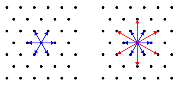
Figure 1: The vector stars of the root systems $A_{2}$ (left) and $G_{2}$ (right). They define neighbouring points in the corresponding root graphs.

In all examples to be discussed below, the generating function is of the form

$$S_{\Lambda}(x)\;=\;\frac{P_{\Lambda}(x)}{(1-x)^{n}}$$ (4)

where $\Lambda$ is a lattice in $n$-dimensional Euclidean space and $P_{\Lambda}(x)$ is an integral polynomial of degree $n$ (for a proof of this statement for the root lattices, see [1]; the remaining cases rest upon the proper generalization of the concept of well-roundedness to root graphs). It is therefore sufficient to list the polynomials in the numerator of (4) for the lattices and graphs under consideration.

Results

Although we shall give the generating functions below, the explicit values of the coordination numbers $s_{\Lambda}(k)$ of root graphs $\Lambda$ in dimension $n\leq 8$ are, for convenience, shown in Table 1 for $1\leq k\leq 10$. Note that, by definition, we set $s_{\Lambda}(0)=1$ in all cases.

Table 1: First coordination numbers of root graphs of dimension $n\leq 8$

$\rule[-5.03749pt]{0.0pt}{15.49994pt}\Lambda$ $s_{\Lambda}(1)$ $s_{\Lambda}(2)$ $s_{\Lambda}(3)$ $s_{\Lambda}(4)$ $s_{\Lambda}(5)$ $s_{\Lambda}(6)$ $s_{\Lambda}(7)$ $s_{\Lambda}(8)$ $s_{\Lambda}(9)$ $s_{\Lambda}(10)$ $A_{1}$ 2 2 2 2 2 2 2 2 2 2 $A_{2}$ 6 12 18 24 30 36 42 48 54 60 $A_{3}$ 12 42 92 162 252 362 492 642 812 1002 $A_{4}$ 20 110 340 780 1500 2570 4060 6040 8580 11750 $A_{5}$ 30 240 1010 2970 7002 14240 26070 44130 70310 106752 $A_{6}$ 42 462 2562 9492 27174 65226 137886 264936 472626 794598 $A_{7}$ 56 812 5768 26474 91112 256508 623576 1356194 2703512 5025692 $A_{8}$ 72 1332 11832 66222 271224 889716 2476296 6077196 13507416 27717948 $B_{2}$ 8 16 24 32 40 48 56 64 72 80 $B_{3}$ 18 74 170 306 482 698 954 1250 1586 1962 $B_{4}$ 32 224 768 1856 3680 6432 10304 15488 22176 30560 $B_{5}$ 50 530 2562 8130 20082 42130 78850 135682 218930 335762 $B_{6}$ 72 1072 6968 28320 85992 214864 467544 918080 1665672 2838384 $B_{7}$ 98 1946 16394 83442 307314 907018 2282394 5095650 10368386 19594106 $B_{8}$ 128 3264 34624 216448 954880 3301952 9556160 24165120 54993792 115021760 $C_{2}$ 8 16 24 32 40 48 56 64 72 80 $C_{3}$ 18 66 146 258 402 578 786 1026 1298 1602 $C_{4}$ 32 192 608 1408 2720 4672 7392 11008 15648 21440 $C_{5}$ 50 450 1970 5890 14002 28610 52530 89090 142130 216002 $C_{6}$ 72 912 5336 20256 58728 142000 301560 581184 1038984 1749456 $C_{7}$ 98 1666 12642 59906 209762 596610 1459810 3188738 6376034 11879042 $C_{8}$ 128 2816 27008 157184 658048 2187520 6140800 15158272 33830016 69629696 $D_{4}$ 24 144 456 1056 2040 3504 5544 8256 11736 16080 $D_{5}$ 40 370 1640 4930 11752 24050 44200 75010 119720 182002 $D_{6}$ 60 792 4724 18096 52716 127816 271908 524640 938652 1581432 $D_{7}$ 84 1498 11620 55650 195972 559258 1371316 2999682 6003956 11193882 $D_{8}$ 112 2592 25424 149568 629808 2100832 5910288 14610560 32641008 67232416 $E_{6}$ 72 1062 6696 26316 77688 189810 405720 785304 1408104 2376126 $E_{7}$ 126 2898 25886 133506 490014 1433810 3573054 7902594 15942206 29896146 $E_{8}$ 240 9120 121680 864960 4113840 14905440 44480400 114879360 265422960 561403680 $F_{4}$ 48 384 1392 3456 6960 12288 19824 29952 43056 59520 $G_{2}$ 12 30 48 66 84 102 120 138 156 174

The coordinator polynomials $P_{\Lambda}(x)$ of the root graphs belonging to the four infinite series turn out to be given by

$$P_{A_{n}}(x) = \sum_{k=0}^{n}\;{\left(\begin{array}[]{@{}c@{}}n\\ k\end{array}\right)}^{2}\;x^{k}$$ (7)

$$P_{B_{n}}(x) = \frac{1}{2}\left[{(1+\sqrt{x})}^{2n+1}+{(1-\sqrt{x})}^{2n+1}\right]\;-\;2nx{(1+x)}^{n-1}$$ (12)

$$= \sum_{k=0}^{n}\;\left[\,\left(\begin{array}[]{@{}c@{}}2n+1\\ 2k\end{array}\right)\>-\>2k\>\left(\begin{array}[]{@{}c@{}}n\\ k\end{array}\right)\,\right]\;x^{k}$$

$$P_{C_{n}}(x) = \frac{1}{2}\left[{(1+\sqrt{x})}^{2n}+{(1-\sqrt{x})}^{2n}\right]\;\;=\;\;\sum_{k=0}^{n}\;\left(\begin{array}[]{@{}c@{}}2n\\ 2k\end{array}\right)\;x^{k}$$ (15)

$$P_{D_{n}}(x) = \frac{1}{2}\left[{(1+\sqrt{x})}^{2n}+{(1-\sqrt{x})}^{2n}\right]\;-\;2nx{(1+x)}^{n-2}$$ (20)

$$= \sum_{k=0}^{n}\;\left[\,\left(\begin{array}[]{@{}c@{}}2n\\ 2k\end{array}\right)\>-\>\frac{2k(n-k)}{n-1}\>\left(\begin{array}[]{@{}c@{}}n\\ k\end{array}\right)\,\right]\;x^{k}\,.$$

In all cases, the coefficients of the polynomials are rather simple expressions in terms of binomial coefficients

$$\left(\begin{array}[]{@{}c@{}}n\\ k\end{array}\right)\;=\;\frac{n!}{k!\,(n-k)!}\>.$$ (21)

The results for the graphs $A_{n}$ ($n\geq 1$) and $D_{n}$ ($n\geq 4$) are just those contained in [1], and the polynomials for $C_{n}$ ($n\geq 2$) can be derived by the methods outlined there, if one observes that the longer roots of $C_{n}$ generate a sublattice that is equivalent to $\mathbb{Z}^{n}$. However, the expressions for $B_{n}$ ($n\geq 2$), as those for $D_{n}$ ($n\geq 4$) here and in [1], are conjectures based on enumeration of coordination sequences for a large number of examples. The striking similarity between $B_{n}$ and $D_{n}$ might actually help to find a proof. The connection is rather intimate: while all roots of $B_{n}$ generate $\mathbb{Z}^{n}$, the long roots alone generate $D_{n}$, and each point of $B_{n}$ can be reached from 0 by using a path with at most one short root.

For the three root graphs related to the exceptional (simply laced) Lie algebras $E_{6}$, $E_{7}$, and $E_{8}$, the coordinator polynomials read

$$P_{E_{6}}(x) = 1+66\,x+645\,x^{2}+1384\,x^{3}+645\,x^{4}+66\,x^{5}+x^{6}$$ (22)

$$P_{E_{7}}(x) = 1+119\,x+2037\,x^{2}+8211\,x^{3}+8787\,x^{4}+2037\,x^{5}$$ (23)

$$\;\;\mbox{}+119\,x^{6}+x^{7}$$

$$P_{E_{8}}(x) = 1+232\,x+7228\,x^{2}+55384\,x^{3}+133510\,x^{4}+107224\,x^{5}$$ (24)

$$\;\;\mbox{}+24508\,x^{6}+232\,x^{7}+x^{8}$$

as has been proved in [1]. Finally, for the two remaining root graphs we find

$$P_{F_{4}}(x) = 1+44\,x+198\,x^{2}+140\,x^{3}+x^{4}$$ (25)

$$P_{G_{2}}(x) = 1+10\,x+7\,x^{2}\>.$$ (26)

Let us give an explicit proof for the last example. Clearly, $s_{G_{2}}(0)=1$ and $s_{G_{2}}(1)=12$. Then, for $n\geq 2$, one can explicitly show that the graph $G_{2}$, in comparison to $A_{2}$ (which also happens to be equivalent to the lattice generated by the long roots of $G_{2}$, see Figure 1), has a shell structure with $s_{G_{2}}(n)=2s_{A_{2}}(n)+s_{A_{2}}(n-1)=18n-6$, from which the above statement follows. By similar arguments, the other examples with short and long root vectors can be traced back to the lattice case; the corresponding shell structure of the root graphis defined by the coordination spheres of its sublattice generated by the set of long root vectors.

Finally, it is interesting to note that the coordination sequences for root graphs $\Lambda$ of type $A_{n}$, $C_{n}$, $D_{n}$, and $E_{6}$ result in self-reciprocal polynomials $P_{\Lambda}(x)$, i.e.,

$$P_{\Lambda}(x)\;=\;x^{n}\cdot P_{\Lambda}(1/x)$$ (27)

while the others do not; for a geometric meaning of this property we refer to [1].

Outlook

We presented the coordination sequences and their generating functions for root lattices and, more generally, graphs based upon the root systems, namely for the series $A_{n}$ ($n\geq 1$), $B_{n}$ ($n\geq 2$), $C_{n}$ ($n\geq 2$), and $D_{n}$ ($n\geq 4$), and for the exceptional cases $E_{6}$, $E_{7}$, $E_{8}$, $F_{4}$, and $G_{2}$. Proofs of various cases can be found in Conway and Sloane [1] or directly based on their results, but the generating functions for $B_{n}$ and $D_{n}$ are still conjectural at the moment.

References

- [1] Conway, J. H.; Sloane, N. J. A.: Low-dimensional lattices VII: coordination sequences. To appear in: Proc. R. Soc. A (1997).
- [2] Galam, S.; Mauger, A.: Universal formulas for percolation thresholds. Phys. Rev. E 53 (1996) 2177–2181.
- [3] Galam, S.; Mauger, A.: A quasi-exact formula for Ising critical temperature on hypercubic lattices. Physica A 235 (1997) 573–576.
- [4] Briggs, K.: Self-avoiding walks on quasilattices. Int. J. Mod. Phys. B 7 (1993) 1569–1575.
- [5] Baake, M.; Grimm, U.; Baxter, R. J.: A critical Ising model on the Labyrinth. Int. J. Mod. Phys. B 8 (1994) 3579–3600.
- [6] Simon, H.; Baake, M.; Grimm, U.: Lee-Yang zeros for substitutional systems. In: Proceedings of the 5th International Conference on Quasicrystals (Eds. C. Janot, R. Mosseri), p. 100–103. World Scientific, Singapore 1995.
- [7] Conway, J. H.; Sloane, N. J. A.: Sphere Packings, Lattices and Groups (2nd ed.). Springer, New York 1993.
- [8] Humphreys, J. E.: Introduction to Lie Algebras and Representation Theory. Springer, New York 1972. And: Reflection Groups and Coxeter Groups. CUP, Cambridge 1990.
- [9] O’Keeffe, M.: -Dimensional Diamond, Sodalite and Rare Sphere Packings. Acta Cryst. A 47 (1991) 748–753.
- [10] O’Keeffe, M.: Coordination sequences for lattices. Z. Kristallogr. 210 (1995) 905–908.
- [11] Sloane, N. J. A.; Plouffe, S.: The Encyclopedia of Integer Sequences. Academic Press, San Diego 1995.
- [12] Sloane, N. J. A.: An on-line version of the encyclopedia of integer sequences. Electronic J. Combinatorics 1 (1994).
- [13] Wilf, H. S.: Generatingfunctionology (2nd ed.). Academic Press, Boston 1994.