Calculations of the Knight Shift Anomalies in Heavy Electron Materials

E. Kim and D. L. Cox1 Department of Physics, Ohio State University, Columbus, OH 43210
Abstract

We have studied the Knight shift $K(\vec{r},T)$ and magnetic susceptibility $\chi(T)$ of heavy electron materials, modeled by the infinite $U$ Anderson model with the NCA method. A systematic study of $K(\vec{r},T)$ and $\chi(T)$ for different Kondo temperatures $T_{0}$ (which depends on the hybridization width $\Gamma$) shows a low temperature anomaly (nonlinear relation between $K$ and $\chi$) which increases as the Kondo temperature $T_{0}$ and distance $r$ increase . We carried out an incoherent lattice sum by adding the $K(\vec{r})$ of a few hundred shells of rare earth atoms around a nucleus and compare the numerically calculated results with the experimental results. For CeSn3, which is a concentrated heavy electron material, both the 119Sn NMR Knight shift and positive muon Knight shift are studied. Also, lattice coherence effects by conduction electron scattering at every rare earth site are included using the average-T matrix approximation. The calculated magnetic susceptibility and 119Sn NMR Knight shift show excellent agreement with experimental results for both incoherent and coherent calculations. The positive muon Knight shifts are calculated for both possible positions of muon (center of the cubic unit cell and middle of Ce-Ce bond axis). Our numerical results show a low temperature anomaly for the muons of the correct magnitude but we can only find agreement with experiment if we take a weighted average of the two sites in a calculation with lattice coherence present. For YbCuAl, the measured 27Al NMR Knight shift shows an anomaly with opposite sign to CeSn3 compound. Our calculations agree very well with the experiments. For the proposed quadrupolar Kondo alloy Y0.8U0.2Pd3, our 89Y NMR Knight shift calculation doesn’t show the observed Knight shift anomaly.

pacs:
74.70.Vy, 74.65.+n, 74.70.Tx

I Introduction

Many heavy electron materials show Knight shift anomalies, which are a deviation from a linear relation of the Knight shift $K(T)$ to the magnetic susceptibility $\chi(T)$ below the Kondo temperature $T_{0}$. The origin of the Knight shift anomalies has been a subject of great interest in the condensed matter community over a period of nearly twenty five years Β [1, 2, 3, 4, 5, 6, 7, 8, 9, 10]. If the impurities in metals have local magnetic moments, they display interesting properties comparing to metals with nonmagnetic impurities, such as a resistivity minimum and anomalies in specific heat and susceptibility. This Kondo effect is a consequence of interaction between the magnetic ion and conduction electron. The central physical concept is that the many body screening cloud surrounding a Kondo impurity site should give rise to an anomalous temperature dependent Knight shift at nuclear sites due to the coupling of the local moment to the nuclear spin through the screening cloudΒ [1, 3, 4, 8, 9]. Such a β€œnon-linear Knight shift anomaly” is to be distinguished from the non-linear susceptibility related to the field dependence of $\chi$. Another way to describe this effect is to say that in the absence of an anomaly, the contribution $K(\vec{r},T)$ from a local moment at distance $\vec{r}$ from the nucleus can be written as $f(\vec{r})\chi(T)$. This factorization does not hold if there is an

anomaly (instead $K(\vec{r},T)=f(\vec{r},T)\chi(T)$ due to the temperature dependent polarization cloud). After HeegerΒ [1] suggested that the anomalous spin cloud was detected at low temperatures, the central question has been whether a conduction electron spin cloud with huge coherence length $\xi_{K}=\hbar v_{F}/k_{B}T_{0}$, where $v_{F}$ is the Fermi velocity and $T_{0}$ is the Kondo temperature exists. The main motivation of this paper is to help clear up this conflict. The Knight shift calculations presented here are the first performed using a realistic impurity model.

This paper is organized as follows. In Sec.Β II, the Kondo effect and the Knight shift anomaly in heavy electron materials will be reviewed. First, general characteristics of the Kondo effect are discussed. We will then review the history of Knight shift anomalies in heavy electron systems. In Sec.Β III, the model Hamiltonian is introduced for both Ce and U compound. Also we review the methods we have used to evaluate the Knight shift (the Non Crossing Approximation(NCA) and average-T matrix approximation (ATA)). Our formalisms for numerical calculations are explained, and a detailed derivation of the Knight shift Feynman diagram will be given in the appendices. In the next section, the numerical results for Ce and Yb ions which are single channel Kondo materials and for U ions in a proposed quadrupolar Kondo alloy will be examined and compared with the experimental results. The calculated NMR Knight shift of Ce and Yb compounds show low temperature anomalies and agree well with the experimental results. But, there is no calculated Knight shift anomaly for the proposed quadrupolar Kondo U compound, in contrast to experiment. The last section includes conclusions and directions for future work.

II Review

A Kondo Effect

The existence of localized moments in dilute alloys that couple to conduction electrons has important consequences for the electrical properties. It has been known since 1930[11] that the resistivity has a rather shallow minimum occurring at a low temperature that depends weakly on the concentration of magnetic impurities instead of dropping monotonically with decreasing temperature like metals with nonmagnetic impurities. In 1963, KondoΒ [12] explained that this minimum arises from some unexpected features of the scattering of conduction electrons off a local magnetic moment, with the simplified model Hamiltonian

β„‹=βˆ‘k→​αϡk→​ck→​α†​ckβ†’β€‹Ξ±βˆ’J2​Nβ€‹βˆ‘k→​kβ†’β€²ck→​α†​σ→α​β​ck→′​α⋅Sβ†’Iβ„‹subscriptβ†’π‘˜π›Όsubscriptitalic-Ο΅β†’π‘˜subscriptsuperscriptπ‘β€ β†’π‘˜π›Όsubscriptπ‘β†’π‘˜π›Όπ½2𝑁subscriptβ†’π‘˜superscriptβ†’π‘˜β€²β‹…subscriptsuperscriptπ‘β€ β†’π‘˜π›Όsubscriptβ†’πœŽπ›Όπ›½subscript𝑐superscriptβ†’π‘˜β€²π›Όsubscript→𝑆𝐼{\cal H}=\sum_{\vec{k}\alpha}\epsilon_{\vec{k}}c^{\dagger}_{\vec{k}\alpha}c_{\vec{k}\alpha}-\frac{J}{2N}\sum_{\vec{k}\vec{k}^{\prime}}c^{\dagger}_{\vec{k}\alpha}\vec{\sigma}_{\alpha\beta}c_{\vec{k}^{\prime}\alpha}\cdot\vec{S}_{I} (1)

where $c_{\vec{k}\alpha}$ is the annihilation operator of the conduction electron, $\alpha$ is the spin index, $\vec{\sigma}$ are Pauli matrices, $\vec{S}_{I}$ is the spin operator of the impurity, and $J<0$ is the exchange coupling. Kondo discovered that the magnetic scattering cross section is divergent in perturbation theory. The anomalously high scattering probability of magnetic ions at low temperatures is a consequence of the dynamic nature of the scattering induced by the exchange coupling and the sharpness of the Fermi surface at low temperatures. Subsequent analysis by Kondo and others has shown that a nonperturbative treatment removes the divergence, yielding instead a term in the impurity contribution to the resistivity that increases with decreasing temperature. In spite of the simple model Hamiltonian, a magnetic $S_{I}=1/2$ local moment interacting with the conduction electron gas, this result is an indication that the problem is explicitly a many body problem, meaning that the electron in state $\vec{k}$ which is being scattered is sensitive to the occupation of all other electron states $\vec{q}$.

For this single channel Kondo model, there is only one characteristic energy scale, the Kondo temperature $T_{0}$, provided that the temperature $T$ is much smaller than the conduction electron bandwidth $D$, and corrections of order $T/D$ are neglected. The Kondo temperature is given by

$$k_{B}T_{0}=D[N(0)J]^{1/2}exp(-1/N(0)J),$$ (2)

where $N(0)$ is the conduction electron density of states at the Fermi level. Any physical quantities are universal functions of $T/T_{0}$. At low temperature, with all material properties buried in $T_{0}$.

This Kondo model can explain the anomalies in the transport coefficients, specific heat and magnetic susceptibility for some alloys with magnetic impurities. The Kondo effect is characterized by the development of the Kondo resonance peak with width of order of $T_{0}$. At high temperatures $T>T_{0}$, the impurity resistivity increases logarithmically as the temperature decreases, and saturates to a finite value at low temperatures below $T<T_{0}$. The magnetic susceptibility has a Curie-Weiss form at high temperatures and shows Pauli paramagnetism at low temperatures with $\chi(T=0)\sim 1/T_{0}$,concomitantly $C/T(T=0)\sim 1/T_{0}$. The $\chi$ behavior is explained by the fact that the magnetic moments which exist at high temperatures are screened out by the conduction electron spin clouds at low temperatures with the formation of a singlet ground state. This conduction spin cloud and the Knight shift anomaly will be discussed more in the next subsection.

B Review of the Knight Shift Anomalies of Heavy Electron Materials

There have been many theoretical and experimental works about the Knight shift anomaly for the heavy electron materials. Whether there is an observable conduction electron spin cloud with huge coherence length has been an issue in condensed matter physics more than 25 years and this is our main motivation to carry out this paper.

In the simplest approximation, the added electron is bound into a singlet with the impurityΒ [13]. Because of the falloff the amplitude of wave function with the energy $\epsilon_{k}$, only states within roughly $\delta k\sim(k_{B}T_{0}/E_{F})k_{F}$ of the Fermi surface are involved in the singlet. As a result, in coordinate space, the singlet wave function extends to a very large distance of order $(\delta k)^{-1}$. Heeger et al.Β [14] calculated the susceptibility at $T=0K$ using the Appelbaum-Kondo theoryΒ [15, 16] and found

$$\chi=\chi_{\mbox{Pauli}}+\chi_{L}+\chi_{Q}$$ (3)

where

$$\chi_{L}=\chi_{Q}=|J|\rho[\mu^{2}/(9/8)k_{B}T_{0}]$$ (4)

Equations (3) and (4) give the very interesting result that one half the excess susceptibility is localized on the impurity site ($\chi_{L}$) and one-half is associated with the partially polarized quasi particle($\chi_{Q}$). The associated spin polarization around the partially magnetized impurity is given by

$$\sigma(r)=\sigma_{0}+\sigma_{RKKY}(r)+\sigma_{Q}(r)$$ (5)

where $\sigma_{0}$ is the uniform polarization due to the external field, $\sigma_{RKKY}(r)$ is the usual RKKY termΒ [17, 18, 19, 20, 21] which $r$ dependence is given by

$$(1/r^{3})\cos(2k_{F}r),$$ (6)

and $\sigma_{Q}(0)$ is the quasiparticle term with

$$<\sigma_{Q}(r)>=<S_{Z}>\frac{3}{2}N\frac{k_{B}T_{0}}{E_{F}}(\frac{\sin k_{F}r}{k_{F}r})^{2}\ln^{2}(r/\xi).$$ (7)

where $\xi_{K}=(2E_{F}/k_{B}T_{0})k_{F}^{-1}$. This expression is valid for $r<\xi_{K}$, and at greater distances $\sigma_{Q}(r)$ rapidly approaches zero. In both the RKKY term and $\sigma_{Q}(r)$ term the value $<S_{Z}>$ is not the free spin value but is determined by the local susceptibility $\chi_{L}$. The existence of the RKKY term for $T<T_{0}$ was shown by SuhlΒ [22].

The technique of nuclear magnetic resonance has been of primary importance in the development of our current understanding of the localized moment problem. The reasons are twofold. First, the nuclei in the host metal in the vicinity of the impurity are sensitive to local perturbations in the spin density(via the hyperfine interaction) and the charge density(via the nuclear quadrupolar interaction). Moreover, the nuclei themselves are only weakly coupled to the electronic system and therefore act as passive ”spies” into the phenomena of interest. Secondly, the nuclear relaxation is sensitive to the low-lying excitations of the electronic system and consequently can provide information on the dynamical aspects of the impurity problem. For the most part NMR experiments in heavy electron compounds are carried out on the nuclei of the non-$f$ ions, so that coupling to the $f$ moments occurs via indirect interactions such as transferred hyperfine and dipolar fields.

The NMR experiment of Boyce and SlichterΒ [2] on Fe impurities in Cu metals showed no evidence for a Knight shift anomaly at low temperature and was interpreted to indicate the absence of this screening cloud or at least a screening cloud of size of the order of a lattice spacing. These mixed results have led to theoretical discussions about the size of any screening conduction electron spin cloud or even whether it existΒ [4, 8, 9, 23, 24, 25].

In contrast, pronounced Knight shift anomalies have been observed in the concentrated heavy electron materials CeSn3[5, 7] and YbCuAl[6, 7], which have been described as Kondo lattice systems with $T_{0}\geq 400K$. In view of the Boyce-Slichter result, the question is raised whether these anomalies represent a coherent effect of the periodic lattice rather than a single ion effect. However, recent experiments on the proposed quadrupolar Kondo alloy[26, 27] Y1-xUxPd3 demonstrate that for concentrations of 0.1-0.2 there are pronounced non-linearities in the Y Knight shift for sufficiently large distances away from the U ion[10].

IshiiΒ [4] calculated the field induced spin polarization for the degenerated Anderson model and confirmed that an anomalous spin cloud is formed outside of the Kondo screening length $\xi_{K}$ at $T\rightarrow 0$. The spin polarization $\sigma(r)$ for electron-hole symmetry case ($\epsilon_{d}=-U/2$) is given by

$$\sigma(r)=\frac{\chi H}{g\mu_{B}}\frac{\cos 2k_{F}r}{4\pi r^{3}}[1-\frac{2E_{F}}{k_{F}r\Delta}\overline{\gamma}].$$ (8)

where $\overline{\gamma}=\chi_{\uparrow\uparrow}$ for $U\rightarrow 0$ and $3/2(2l+3)\chi_{\uparrow\uparrow}$ for $U\rightarrow\infty$, where $l$ is the orbital angular momentum. $\chi_{\uparrow\uparrow}$ changes from $(g\mu_{B})^{2}/2\pi\Gamma$ for $U=0$ to $(g\mu_{B})^{2}S(S+1)/3k_{B}T_{0}$ for $s-d$ Exchange model ($U=\infty$). Therefore the coherence length $\xi_{K}=2E_{F}/k_{F}\Delta\overline{\gamma}$ varies from $2\hbar v_{F}/\Gamma$ at $U=0$ to $2\pi\hbar v_{F}/3k_{B}T_{0}$ in the $s-d$ limit. Also, for the strong $U/\pi\Gamma$ limit, spin polarization is calculated for $r<\xi_{K}$. It is given by

$$\sigma(r)=\frac{4\Gamma}{\pi U}\frac{\chi H}{g\mu_{B}}\frac{\cos 2k_{F}r}{4\pi r^{3}}.$$ (9)

By the relation $4V^{2}/U=-J/2N$Β [28], the above spin polarization is just the RKKY contribution. Comparing the equations (8) and (9), the conduction electron spin cloud which is formed outside the Kondo coherence length has the RKKY form but with $2N/N(0)J$ times bigger amplitude than the spin cloud inside the Kondo coherence length.

Chen et al.Β [8] calculated the zero frequency response function $C(\vec{r},T)$ around a magnetic impurity, using a perturbative thermodynamic scaling procedure and nonperturbative renomalization group method for $S=1/2$ Kondo model. The host nuclei near magnetic impurities at positions $\vec{r}$ displays satellite resonances in the tail of the main magnetic resonance signal, with a Knight shift given by $K+\Delta K(\vec{r})$, where $K=\rho_{0}g_{e}/2$ is the Knight shift of the pure host. Then $\Delta K$ is

$$\Delta K=C(\vec{r},T)-K$$ (10)

Chen et al.Β [8] showed that this Knight shift is factorized into a product of temperature and spatial dependent functions, specifically

$$\Delta K=F(\vec{r})\chi(T)$$ (11)

where $\chi(T)$ is the magnetic susceptibility. The computed $F(r)$ has the RKKY form.

The conduction electron spin polarization in the Anderson model has been studied with the NCA previously by W. Pollwein et al.Β [9]. However, this study was carried out only for the spin 1/2 model with infinite Coulomb repulsion, and for a limited parameter regime (only results for very low $T_{0}$ values and short distances $(r\ll\xi_{K})$ have been numerically calculated). In consequence, no strong evidence was found for a Knight shift anomaly in this previous work.

Recently, E. SΓΈrensen and I. AffleckΒ [23, 24, 25] showed that the Kondo coherence length $\xi_{K}=\hbar v_{F}/k_{B}T_{0}$, varies when temperature changes by combining a finite size scaling ansatz with density matrix renomalization group calculations. They write the scaling hypothesis for three dimensional susceptibility is

$\displaystyle\chi_{\mbox{imp}}(r)$ $\displaystyle=$ $\displaystyle\chi-\rho/2$ (12)
$\displaystyle=$ $\displaystyle\frac{\cos(2k_{F}r)}{8\pi^{2}v_{F}r^{2}}f(rT/v_{F},T/T_{0})$ (14)
$\displaystyle(\mbox{for }r\gg 1/k_{F};T,T_{0}\ll E_{F}),$

where $f$ is a real universal scaling function. $\rho/2$ is the standard Pauli bulk susceptibility with $\rho$ the density of states per spin. At higher temperatures $T>T_{0}$, the local susceptibility shows RKKY behavior and at lower temperatures $T<T_{0}$ it has a local Fermi liquid form. So the Knight shift has longer range at low temperatures where the conduction electron screening cloud has formed than at high temperatures where it has not. Sorensen and Affleck tried to explain the experiment by Boyce and SlichterΒ [2] by the possible factorization of the scaling functions deep inside the screening cloud where the experiment was done.

III Model and Formalism

A Model Hamiltonian

In our work, we use the on-site Coulomb interaction $U=\infty$ single impurity Anderson modelΒ [29]. The Anderson model can be canonically transformed by the Schrieffer-Wolff transformation to the Kondo model at $U=\infty$ limitΒ [28], and is a good model Hamiltonian to describe heavy electron materials with $f$ electrons. Schematics of this model are shown in FigΒ 1 for Ce ions. This $U=\infty$ model can be a good approximation in the limit when the ratio of the virtual $4f$ level width $\Gamma$ to the on site Coulomb repulsion $U$ is small. For real materials this interaction energy is of the order of $U=5eV$Β [30, 31], and the hybridization width is of the order of $\Gamma=0.1eV$. For Ce(Yb) ions, we keep $f^{0}$ and $f^{1}(f^{14}$ and $f^{13})$ configurations, and for U ions, which are proposed two channel quadrupolar Kondo alloys, we keep $f^{2}$ and $f^{3}$ configurations. For Ce and Yb ions, spin orbit coupling is included and for U ions, spin orbit coupling and also crystal field splittings are included. The crystal electric field(CEF) will split the spin-orbit multiplet and can mix two different angular momentum multiplets($j$, $j^{\prime}$). But the correction of the mixing term between two different $j$’s by CEF is small, we only consider the splitting effect. These crystal electric field effects in the Anderson model were first considered by HirstΒ [32] based on group theory and it will be discussed more in the AppendixΒ B.

We shall first discuss the situation for Ce3+ and Yb3+ ions, and write down the model only for the Ce case(the Yb3+ ion has a lone $4f$ hole and our procedure describes this with a simple particle hole transformation).

For a single Ce site at the origin, the model is

$${\cal H}={\cal H}_{c}+{\cal H}_{f}+{\cal H}_{cf}+{\cal H}_{z}$$ (15)

with

β„‹c=βˆ‘k→​σϡk​ck→​σ†​ck→​σsubscriptℋ𝑐subscriptβ†’π‘˜πœŽsubscriptitalic-Ο΅π‘˜subscriptsuperscriptπ‘β€ β†’π‘˜πœŽsubscriptπ‘β†’π‘˜πœŽ{\cal H}_{c}=\sum_{\vec{k}\sigma}\epsilon_{k}c^{\dagger}_{\vec{k}\sigma}c_{\vec{k}\sigma} (16)

the conduction band term for electrons with a broad featureless density of states of width $D$, taken to be Lorentzian here for convenience, with

$${\cal H}_{f}=\sum_{jm_{j}}\epsilon_{fj}|f^{1}jm_{j}\rangle\langle f^{1}jm_{j}|$$ (17)

where $j=5/2,7/2$ indexes the angular momentum multiplets of the Ce ion having azimuthal quantum numbers $m$, with $\epsilon_{f5/2}=-2eV$,Ο΅f​7/2=Ο΅f​5/2+Ξ”s​o=βˆ’1.71​e​Vsubscriptitalic-ϡ𝑓72subscriptitalic-ϡ𝑓52subscriptΞ”π‘ π‘œ1.71𝑒𝑉\epsilon_{f7/2}=\epsilon_{f5/2}+\Delta_{so}=-1.71eV (we take the $f^{0}$ configuration at zero energy), with

$${\cal H}_{cf}={\sum_{\vec{k}jm\sigma}}[\;V_{\vec{k}j\sigma m_{j}}c^{\dagger}_{\vec{k}\sigma}|f^{0}0\rangle\langle f^{1}jmi_{j}|+h.c.\>]$$ (18)

where $V_{\vec{k}j\sigma m_{j}}=VY_{3m_{j}-\sigma}(\hat{k})\langle 3m_{j}-\sigma,1/2\sigma|jm_{j}\rangle/\sqrt{N_{s}}$, $V$ being the one particle hybridization strength and $N_{s}$ the number of sites. We can rewrite the hybridization Hamiltonian as

$${\cal H}_{cf}={\sum_{kjm_{j}}}[\;V_{k}c^{\dagger}_{\vec{k}jm_{j}}|f^{0}0\rangle\langle f^{1}jm_{j}|+h.c.\>]$$ (19)

where

ck​j​mj†=βˆ‘mβ€‹ΟƒβŸ¨3​m​12​σ|j​mjβŸ©β€‹ck​m​σ†subscriptsuperscriptπ‘β€ π‘˜π‘—subscriptπ‘šπ‘—subscriptπ‘šπœŽinner-product3π‘š12πœŽπ‘—subscriptπ‘šπ‘—subscriptsuperscriptπ‘β€ π‘˜π‘šπœŽc^{\dagger}_{kjm_{j}}=\sum_{m\sigma}\langle 3m\frac{1}{2}\sigma|jm_{j}\rangle c^{\dagger}_{km\sigma} (20)

with $c_{km\sigma}=k\int d\hat{k}Y^{*}_{3m}(\hat{k})c_{\vec{k}\sigma}$. For the Yb case, the hybridization Hamiltonian is given by

$${\cal H}_{cf}={\sum_{kjm_{j}}}[\;V_{k}c^{\dagger}_{kjm_{j}}|f^{13}j-m_{j}\rangle\langle f^{14}0|+h.c.\>].$$ (21)

${\cal H}_{z}$, the Zeeman energy of the electronic system for a magnetic field $H_{z}$ applied along the $z$-axis is given by

$${\cal H}_{z}=-\mu_{B}H_{z}[2\sum_{\vec{k}\sigma}\sigma n_{\vec{k},\sigma}-\sum_{jm}g_{j}m|f^{1}jm\rangle\langle f^{1}jm|\>].$$ (22)

In addition to this, we must add a term coupling the nuclear spin system to the conduction electrons, which we take to be of a simple contact form $\sim\vec{I}(\vec{r})\cdot\vec{S}(\vec{r})$ for each nuclear spin $\vec{I}(\vec{r})$ at position $\vec{r}$ with $\vec{S}(\vec{r})$ the conduction spin density at the nuclear site, and a nuclear Zeeman term. In terms of the parameters, the Kondo scale characterizing the low energy physics is given by

kB​T0=D​(Γπ​|Ο΅f|)1/Ng​(DΞ”s​o)Ne​x/Ng​exp⁑(π​ϡfNg​Γ)subscriptπ‘˜π΅subscript𝑇0𝐷superscriptΞ“πœ‹subscriptitalic-ϡ𝑓1subscript𝑁𝑔superscript𝐷subscriptΞ”π‘ π‘œsubscript𝑁𝑒π‘₯subscriptπ‘π‘”πœ‹subscriptitalic-ϡ𝑓subscript𝑁𝑔Γk_{B}T_{0}=D(\frac{\Gamma}{\pi|\epsilon_{f}|})^{1/N_{g}}(\frac{D}{\Delta_{so}})^{N_{ex}/N_{g}}\exp(\frac{\pi\epsilon_{f}}{N_{g}\Gamma}) (23)

where the single particle hybridization width $\Gamma=\pi N(0)V^{2}$ with $N(0)$ which is the density of the states at the Fermi energy. Other parameters are defined in TableΒ I.

For the $Y_{1-x}U_{x}Pd_{3}$ which has the cubic AuCu3 structure, the crystal field effect (CEF) must be included. This crystal electric field effects lift the angular momentum degeneracy of U ions and their spin-orbit multiplet decomposes into irreducible representation of the cubic field. The $f^{2},j=4$ Hund’s rule ground state of U compound is split to a $\Gamma_{3}$ nonmagnetic doublet, $\Gamma_{5}$ and $\Gamma_{4}$ magnetic triplet and $\Gamma_{1}$ singlet states[33]. And $f^{3},j=9/2$ spin-orbit multiplet is split to $\Gamma_{7}$ doublet and two $\Gamma_{8}$ quartets. In our calculation we choose $j=4$ $\Gamma_{3}$ for the ground state for $f^{2}$ configuration and $j=9/2$ $\Gamma_{6}$ for the ground state of the $f^{3}$ configuration. Fig.Β 2 shows the schematic configuration diagram. All parameter values are listed in TableΒ II in the unit of $D$. For an explicit derivation of Hamiltonian for U ions, see the AppendixΒ A.

B Non Crossing Approximation

We treat the Anderson Hamiltonian with the non-crossing approximation (NCA), a self- consistent diagrammatic perturbation theory discussed at length in the paper of Bickers et al.[34]. This is useful because this method provides ways of calculating the dynamic response functions, such as the one electron Green’s functions and dynamic susceptibility and it makes possible a more extensive comparison between the theoretical predictions and experimental results.

In the NCA, we do the $1/N$ expansions with the new variable $N$, the large orbital degeneracy of the ground state of $f$ electrons. These simple approximation schemes work very well for values of $N$ that are of interest in applications to rare earth impurities. For example, the lowest spin-orbit split multiplet for Ce 4$f^{1}$ has $j=5/2$, corresponding to $N=6$, and for Yb $4f^{13}$, $j=7/2$, corresponding to $N=8$. Even for $N=2$ one can get good semi-quantitative results, which can be accurate to within a few percent for some quantities.

It was noted that, in a perturbative $1/N$ expansion, the $f$-electron spectral density exhibits a singularity at $\omega=T_{0}$, with $T_{0}\simeq D\exp(\pi\epsilon_{f}/N\Gamma)$. This singularity remains order by order, preventing a complete description of $f$ photoemission and electronic transport. In order to remove this singularity, it is necessary to perform an infinite-order resummation in $1/N$ Β [34, 36, 37, 38, 39, 40, 41, 42, 43, 44, 45, 46, 47].

In the NCA , our starting basis is the conduction band plus the atomic Hamiltonian projected to the atomic electron Fock space and treat the hybridization between the conduction band and the atomic orbital as a perturbation. The strength of this approach is that the strong on-site Coulomb interaction for atomic electrons is included at the outset. The conventional Feynman diagram technique which uses Wick’s theorem can not be applied for strongly correlated problems with restricted Hilbert spaces. Pseudo particle Green’s functions are introduced for each atomic electron occupation state which is neither fermionic nor bosonic (i.e., $f^{1}$ $j=5/2$, $7/2$ and $f^{0}$ in the present model for Ce ions). The pseudo fermion Green’s functions for $f^{1}$ $j=5/2$, $7/2$ angular momentum multiplets are

$$G_{jm}(z)=\frac{1}{z-\epsilon_{fj}-\Sigma_{jm}(z)}$$ (24)

and the pseudo boson Green’s function for the $f^{0}$ is

$$D(z)=\frac{1}{z-\Sigma_{0}(z)}.$$ (25)

Then we insert a self-energy into the propagators of pseudo particles. This gives coupled integral equations for the ionic propagator self energies, $\Sigma_{0}(z)$, $\Sigma_{jm}(z)$. ΒΏFrom the leading order diagrams of Fig.Β 3, the coupled equations for the self energies are

$\displaystyle\Sigma_{0}(z)$ $\displaystyle=$ $\displaystyle V^{2}\sum_{j}N_{j}\sum_{k}\frac{f_{k}}{z+\epsilon_{k}-\epsilon_{fjm}-\Sigma_{jm}(z+\epsilon_{k})}$ (26)
$\displaystyle=$ $\displaystyle V^{2}\sum_{j}N_{j}\sum_{k}f_{k}G_{jm}(z+\epsilon_{k})$ (27)
$\displaystyle\Sigma_{jm}(z)$ $\displaystyle=$ $\displaystyle V^{2}\sum_{k}\frac{1-f_{k}}{z-\epsilon_{k}-\Sigma_{0}(z-\epsilon_{k})}$ (28)
$\displaystyle=$ $\displaystyle V^{2}\sum_{k}(1-f_{k})D(z-\epsilon_{k}),$ (29)

where $V$ is the hybridization strength between the conduction band and the atomic orbitals and $N_{j}$ is the degeneracy of the spin-orbit multiplet $j$. It is convenient to introduce the spectral functions $A_{jm}(\omega)$,and $B(\omega)$ for pseudo-particle Green’s functions.

$\displaystyle G_{jm}(i\omega)$ $\displaystyle=$ $\displaystyle\int\frac{d\rho}{\pi}\frac{A_{jm}(\rho)}{i\omega-\rho}$ (30)
$\displaystyle A_{jm}(\omega)$ $\displaystyle=$ $\displaystyle-\mbox{Im}\;G_{jm}(\omega)$ (31)
$\displaystyle D(i\nu)$ $\displaystyle=$ $\displaystyle\int\frac{d\zeta}{\pi}\frac{B(\zeta)}{i\nu-\zeta}$ (32)
$\displaystyle B(\nu)$ $\displaystyle=$ $\displaystyle-\mbox{Im}\;D(\nu)$ (33)

In addition to spectral functions $A_{jm}(\rho)$ and $B(\zeta)$, it is necessary to introduce negative frequency spectral functions $A_{jm}^{(-)}(\rho)$ and $B^{(-)}(\zeta)$. These spectra are given by

$\displaystyle A_{jm}^{(-)}(\rho,T)$ $\displaystyle=$ $\displaystyle A_{jm}(\rho,T)e^{-\beta(\rho-E_{0})}$ (34)
$\displaystyle B^{(-)}(\zeta,T)$ $\displaystyle=$ $\displaystyle B(\zeta,T)e^{-\beta(\zeta-E_{0})},$ (35)

where $E_{0}$ is the ground state energy relative to the Fermi energy. The impurity partition function $Z_{4f}$ is given by

$\displaystyle Z_{4f}(T)$ $\displaystyle=$ $\displaystyle\int\frac{d\zeta}{\pi}[\sum_{jm}A_{jm}(\zeta,T)+B(\zeta,T)]e^{-\beta\zeta}.$ (36)
$\displaystyle=$ $\displaystyle e^{-\beta E_{0}}\int\frac{d\zeta}{\pi}[\sum_{jm}A_{jm}^{(-)}(\zeta,T)+B^{(-)}(\zeta,T)].$ (37)

At $T\rightarrow 0$, $Z_{4f}(T)$ becomes

$$Z_{4f}(0)=e^{-\beta E_{0}}.$$ (38)

The iteration of these coupled equations for the self energies generates a set of diagrams which includes all non-crossing diagrams, but does not correspond to any specific order in the $1/N$ expansion by treating $NV^{2}$ as ${\it O}(1))$ where $V$ is the hybridization strength between the conduction electron and the atomic orbitals. The set of diagrams summed by these equations includes all the terms of order ${\it O}(1)$ and ${\it O}(1/N)$ and a subset of contributions from the higher order terms. The lowest order skeleton diagrams which are not included are of order ${\it O}(1/N^{2})$. All the diagrams that enter at ${\it O}(1)$ and ${\it O}(1/N)$ have non-crossing conduction lines. Specifically, the leading order vertex corrections, which are ${\it O}(1/N^{2})$, are not included in the NCA.

These self-consistent integral equations are solved to second order in the hybridization for the ionic propagator self energies. Then physical properties, such as the resistivity and magnetic susceptibility $\chi$, are calculated as convolutions of these propagators. Fig.Β 4 shows a leading order Feynman diagram for the static magnetic susceptibility and its convolution integral is given by Eq. (39). This is discussed more in section Β III C.

The NCA shows a pathological behavior (due to the truncation of the diagrammatic expansion) for a temperature scale $T_{p}\ll T_{0}$ in this conventional Anderson model. However, provided the $f^{1}$ occupancy $n_{f}\geq 0.7$, and $N\geq 4$, this is not a problem, as shown in Ref.Β [34], in that comparison of NCA results with exact thermodynamics from the Bethe-Ansatz shows agreement at the few percent level above $T_{p}$. Hence, this is a reliable method for our purposes.

Our numerical procedure, briefly, consists of solving the NCA integral equations for the Anderson Hamiltonian specified above on a logarithmic mesh with order 600 points chosen to be centered about the singular structures near the ground state energy $E_{0}\sim\epsilon_{f5/2}$. We then feed the self-consistent propagators for the empty and singly occupied orbitals into the convolution integrals obtained from the diagram of Fig.Β  5, which allows for evaluation of the Knight shift at arbitrary angle and distance from the nuclear site. This will be explained more in sectionΒ III D. It is convenient to take the nuclear site as the origin in this case leading to phase factors $e^{-i\vec{k}\cdot R}$ in the hybridization Hamiltonian ${\cal H}_{cf}$, where $\vec{r}$ is the nuclear-Ce site separation. These factors give the oscillations and position space angular dependence in the Knight shift $K$.

C Magnetic Susceptibility

The static magnetic susceptibility is a direct indicator of the nature of the ground state for the Kondo and Anderson model. Near room temperature, the susceptibility $\chi(T)$ displays a Curie-Weiss temperature dependence for most heavy-electron materials. $\chi$ is linearly related to the Knight shift $K(T)$. At low temperature, $\chi(T)$ does not follow the Curie-Weiss law and for some systems, a linear relation of the Knight shift $K(T)$ to the magnetic susceptibility breaks down and hence shows a Knight shift anomaly.

In general the magnetic susceptibility comes from self-correlation of the conduction band magnetization($\chi_{cc}$), the self-correlation of the $f$ magnetization($\chi_{ff}$), and the mutual correlation of $f$ and band components($\chi_{cf}$). The leading diagram comes from the second term where the only $f$ electrons are coupled to the field and this gives a good approximation to the overall susceptibility. This diagram for magnetic susceptibility is in Fig.Β 4. Then, in the NCA, the magnetic susceptibility in the zero field limit can be writtenΒ [35]

$$\chi(T)=\sum_{j}\frac{\mu_{j}^{2}N_{j}}{Z_{4f}(T)}2\int\frac{d\zeta}{\pi}A_{jm}^{(-)}(\zeta,T)\mbox{Re}G_{jm}(\zeta,T)$$ (39)

where $\mu_{j}$ is the effective magnetic moment which is defined as $\mu_{j}^{2}=(g_{j}\mu_{B})^{2}j(j+1)/3$ where $g_{j}$ is the LandΓ© g𝑔g factor for the $j$ multiplet and $Z_{4f}(T)$ is the impurity partition function.

Also we can get the van Vleck magnetic susceptibility between $j$ and $j^{\prime}$ angular momentum multiplet.

$\displaystyle\chi^{{}^{\prime\prime}}_{m_{j}m_{j^{\prime}}}(\omega)$ $\displaystyle=$ $\displaystyle\mu_{B}^{2}\frac{|\langle jm_{j}|J_{z}+S_{z}|j^{\prime}m_{j^{\prime}}\rangle|^{2}}{Z_{4f}(T)}(1-e^{-\beta\omega})$ (41)
$\displaystyle\times\int\frac{d\zeta}{\pi}A_{jm_{j}}(\zeta+\omega)A_{j^{\prime}m_{j^{\prime}}}^{(-)}(\zeta)$

With $\langle\frac{5}{2},m|J_{z}+S_{z}|\frac{7}{2},m^{\prime}\rangle=-(\sqrt{49-4m^{2}}/14)\delta_{mm^{\prime}}$, the total van Vleck susceptibility for $j=5/2$ and $j^{\prime}=7/2$ is

$\displaystyle\chi_{vv}^{{}^{\prime\prime}}(\omega)$ $\displaystyle=$ $\displaystyle\sum_{m_{j},m_{j^{\prime}}}\chi_{m_{j}m_{j^{\prime}}}^{{}^{\prime\prime}}(\omega)$ (43)
$\displaystyle=$ $\displaystyle\frac{8}{7}\mu_{B}^{2}\frac{(1-e^{-\beta\omega})}{Z_{4f}(T)}\int\frac{d\zeta}{\pi}A_{jm}(\zeta+\omega)A_{j^{\prime}m}^{(-)}(\zeta).$ (44)

The susceptibility sum rule is derived from the zero frequency limit of the Hilbert transform of $\chi_{vv}^{{}^{\prime\prime}}(\omega,T)$,

$$\chi_{vv}(T)=\chi^{\prime}_{vv}(0,T)=\int\frac{d\omega}{\pi}\frac{\chi^{{}^{\prime\prime}}_{vv}(\omega,T)}{\omega}$$ (45)

In our calculation, both the $j=5/2$, $7/2$ contributions to the static magnetic susceptibility and the van Vleck susceptibility are considered for Ce ions. For Yb ions, only the static susceptibility of the $j=7/2$ ground spin-orbit multiplet is calculated because that the energy gap between two spin orbit multiplets ($j=7/2$ and $j=5/2$) is large ( about $1.2eV$) For Y1-xUxPd3, only the van Vleck susceptibility between different $\Gamma$ states is calculated because the assumed $\Gamma_{3}$ ground state is a non-magnetic doublet.

D Knight Shift

Knight shift measurements on the nuclear spins of non-$f$ ions in Kondo or heavy electron materials can probe the local induced magnetic fields. The additional fields come from all the possible polarization sources, such as conduction electron spin polarization. For $f$ electrons, the radius wave function is small and they are well screened, so there is little possibility of direct overlap interactions between the nuclear spins and local moments. In particular, the polarization of conduction electrons by the polarized local Kondo impurities, i.e. the transferred $f$-electron polarization, is usually expected to have the most significant temperature dependent contribution.

The Knight shift of Heavy electron materials is induced by the indirect interactions of the magnetic impurity and host nuclear spin mediated by the conduction electrons. Without the charge fluctuations introduced by the hybridization interaction between conduction electron and $f$ electron, this indirect interaction has the RKKY interaction form. So at high temperatures, the Knight shift follows the RKKY interaction and at low temperatures where the Kondo effect appears, the Knight shift can show deviation from the RKKY form.

To calculate the Knight shift we need to evaluate the Feynman diagram in FigΒ 5 which is the lowest order diagram coupling the nuclear spin to, say, Ce magnetic moments, ignoring direct Coulomb exchange coupling. All the propagator symbols are explained in the figure. For the incoherent calculation, the conduction electrons are assumed to belong to a broad, featureless, and symmetric band of half width $D$. The conduction electron propagator is taken to be a bare electron propagator, i.e. it includes no self energy effects reflecting multiple scattering off the $f$-sites. When the the lattice coherence effects of conduction electrons are included, the self energy arising from the scattering of conduction electron at every $f$ site is included in the conduction electron propagator in an approximate way.

The Knight shift for a nuclear spin or muon at $\vec{r}$ is approximated as

$\displaystyle K(r,\theta)$ $\displaystyle=$ $\displaystyle-\frac{8\pi V^{2}}{3N_{s}}\frac{g_{e}\mu^{2}_{B}}{\Omega}\sum f_{jj^{\prime}}(\alpha,\theta)\int k^{2}\,dk$ (47)
$\displaystyle\times\int k^{\prime 2}\,dk^{\prime}I_{jj^{\prime}}(\epsilon_{k},\epsilon_{k^{\prime}}),$

where $g_{e}$ is the electron $g$-factor and $\mu_{B}$ is the Bohr magneton. Here $\theta$ is the angle between $z$ axis and the bond direction $\vec{r}$ which connects the nucleus or muon to a given $f$ ion in the crystal and $\alpha$ is the angle between the field axis and bond axis. $I_{jj^{\prime}}(\epsilon_{k},\epsilon_{k^{\prime}})$ is given by

$\displaystyle I_{jj^{\prime}}(\epsilon_{k},\epsilon_{k^{\prime}})$ $\displaystyle=$ $\displaystyle j_{3}(kr)j_{3}(k^{\prime}r)\frac{1}{Z_{4f}}\sum_{\omega,\nu}G_{0}(k\sigma,i\omega)G_{0}(k^{\prime}\sigma^{\prime},i\omega)$ (49)
$\displaystyle\times G_{jm}(i(\omega+\nu))G_{j^{\prime}m^{\prime}}(i(\omega+\nu))D(i\nu)$
$\displaystyle=$ $\displaystyle 2\;\frac{j_{3}(kr)j_{3}(k^{\prime}r)}{\epsilon_{k}-\epsilon_{k^{\prime}}}(f(\epsilon_{k})I_{1jj^{\prime}}(\epsilon_{k})$ (51)
$\displaystyle+(1-f(\epsilon_{k}))I_{2jj^{\prime}}(\epsilon_{k})),$

where

$\displaystyle I_{1jj^{\prime}}(\epsilon_{k})$ $\displaystyle=$ $\displaystyle\frac{2}{Z_{4f}}\!\int\!\frac{d\zeta}{\pi}\int\!\frac{d\rho}{\pi}\frac{(B^{(-)}(\zeta)A_{jm}(\rho)\mbox{Re}G_{j^{\prime}m^{\prime}}(\rho)}{\epsilon_{k}+\zeta-\rho}$ (52)
$\displaystyle=$ $\displaystyle\frac{1}{Z_{4f}}\!\int\!\frac{d\zeta}{\pi}B^{(-)}(\zeta)\mbox{Re}G_{jm}(\zeta+\epsilon_{k})$ (54)
$\displaystyle\;\;\;\;\times\mbox{Re}G_{j^{\prime}m^{\prime}}(\zeta+\epsilon_{k})$
$\displaystyle I_{2jj^{\prime}}(\epsilon_{k})$ $\displaystyle=$ $\displaystyle\frac{-2}{Z_{4f}}\!\int\!\frac{d\rho}{\pi}\int\!\frac{d\zeta}{\pi}\frac{B(\zeta)A_{jm}^{(-)}(\rho)\mbox{Re}G_{j^{\prime}m^{\prime}}(\rho))}{\epsilon_{k}+\zeta-\rho}$ (55)
$\displaystyle=$ $\displaystyle\frac{2}{Z_{4f}}\!\int\!\frac{d\rho}{\pi}A_{jm}^{(-)}(\rho)\mbox{Re}G_{j^{\prime}m^{\prime}}(\rho)\mbox{Re}D(\rho-\epsilon_{k}).$ (56)

The derivation is explained in detail in AppendixΒ C.

We can analytically evaluate the inner $k^{\prime}$ integral as

$$\int_{0}^{\infty}k^{\prime 2}\;dk^{\prime}\frac{j_{3}(k^{\prime}r)}{k^{2}-k^{\prime 2}},$$ (57)

and the results are presented in AppendixΒ D.

For a magnetic field in the $z$ direction (i.e., $\theta=\alpha)$, and for $I=1/2$, the angular dependent function in the Knight shift, $f_{jj^{\prime}}(\alpha,\theta)$, is given by

$$f_{jj^{\prime}}(\theta)=\cos^{2}\theta f_{jj^{\prime}}^{z}+\frac{\sin^{2}\theta}{4}(f^{1-}_{jj^{\prime}}+f^{2-}_{jj^{\prime}}+f^{1+}_{jj^{\prime}}+f^{2+}_{jj^{\prime}}).$$ (58)

Here $f^{z}_{jj^{\prime}}(\theta)$ is

$\displaystyle f_{jj^{\prime}}^{z}(\theta)$ $\displaystyle=$ $\displaystyle\sum_{m_{j},m_{j^{\prime}}}\langle jm_{j}|J_{z}+S_{z}|j^{\prime}m_{j^{\prime}}\rangle\sigma^{z}_{\alpha\alpha}\langle j^{\prime}m_{j^{\prime}}|\hat{r}\rangle\langle\hat{r}|jm_{j}\rangle$ (59)
$\displaystyle=$ $\displaystyle\sum_{m_{j},\alpha,m_{3}}\alpha\langle jm_{j}|J_{z}+S_{z}|j^{\prime}m_{j^{\prime}}\rangle\langle j^{\prime}m_{j^{\prime}}|3m_{3};\frac{1}{2}\alpha\rangle$ (61)
$\displaystyle\times\langle 3m_{3};\frac{1}{2}\alpha|jm_{j}\rangle|Y_{3m_{3}}(\hat{r})|^{2}.$

and $f^{1\pm}_{jj^{\prime}}(\theta)$ and $f^{2\pm}_{jj^{\prime}}(\theta)$ are

$\displaystyle f^{1\pm}_{jj^{\prime}}(\theta)$ $\displaystyle=$ $\displaystyle\sum_{m_{j}m_{j^{\prime}}\alpha,\beta}\langle j,m_{j}|J_{\pm}|j^{\prime},m_{j^{\prime}}\rangle\langle j^{\prime}m_{j^{\prime}}|\hat{r}\rangle\sigma^{\mp}_{\alpha\beta}\langle\hat{r}|j,m_{j}\rangle$ (62)
$\displaystyle=$ $\displaystyle\sum_{m_{j},m_{j^{\prime}},m_{3},m^{\prime}_{3},\alpha,\beta}\!\!\!\langle j,m_{j}|J_{\pm}|j^{\prime},m_{j^{\prime}}\rangle\langle j^{\prime}m_{j^{\prime}}|3m^{\prime}_{3};\frac{1}{2}\alpha\rangle$ (65)
$\displaystyle\times\langle 3m^{\prime}_{3};\frac{1}{2}\alpha|\sigma^{\mp}_{\alpha,\beta}|3m_{3};\frac{1}{2}\beta\rangle\langle 3m_{3};\frac{1}{2}\beta|jm_{j}\rangle$
$\displaystyle\times Y^{*}_{3m_{3}}(\hat{r})Y_{3m^{\prime}_{3}}(\hat{r})$
$\displaystyle f^{2\pm}_{jj^{\prime}}(\theta)$ $\displaystyle=$ $\displaystyle\sum_{m_{j}m_{j^{\prime}}\alpha\beta}\langle jm_{j}|S_{\pm}|j^{\prime},m_{j^{\prime}}\rangle\langle j^{\prime}m_{j^{\prime}}|\hat{r}\rangle\sigma^{\mp}_{\alpha\beta}\langle\hat{r}|j,m_{j}\rangle$ (66)
$\displaystyle=$ $\displaystyle\sum_{m_{j},m_{j^{\prime}},m_{3},m^{\prime}_{3},\alpha,\beta}\!\!\!\langle j,m_{j}|S_{\pm}|j^{\prime},m_{j^{\prime}}\rangle\langle j^{\prime}m_{j^{\prime}}|3m^{\prime}_{3};\frac{1}{2}\alpha\rangle$ (69)
$\displaystyle\times\langle 3m^{\prime}_{3};\frac{1}{2}\alpha|\sigma^{\mp}_{\alpha,\beta}|3m_{3};\frac{1}{2}\beta\rangle\langle 3m_{3};\frac{1}{2}\beta|jm_{j}\rangle$
$\displaystyle\times Y^{*}_{3m_{3}}(\hat{r})Y_{3m^{\prime}_{3}}(\hat{r})$

The explicit values for $f_{jj^{\prime}}(\theta)$ are

$\displaystyle f_{\frac{5}{2}\frac{5}{2}}(\theta)$ $\displaystyle=$ $\displaystyle\frac{9}{28\pi}(1-8\sin^{2}\theta+6\sin^{4}\theta)$ (70)
$\displaystyle f_{\frac{7}{2}\frac{7}{2}}(\theta)$ $\displaystyle=$ $\displaystyle\frac{2}{7\pi}[2+12\sin^{2}\theta-9\sin^{4}\theta]$ (71)
$\displaystyle f_{\frac{5}{2}\frac{7}{2}}(\theta)$ $\displaystyle=$ $\displaystyle\frac{3}{28\pi}[4-4\sin^{2}\theta+3\sin^{4}\theta].$ (72)

To assess the relevance of this single site physics to the periodic compound CeSn3, we also carried out incoherent lattice sums over a few hundred radial shells of Ce atoms around the Sn nucleus. For each atom in a shell the distance $r$ and angle $\theta$ of Ce ion is calculated and the Knight shift of each ion is evaluated for given position. Then the contribution from each ion is added to get the total Knight shift. For the Y1-xUxPd3, impurity configuration averaging is also carried out. This single site physics is known to be a good approximation at high temperatures where the ions are incoherent with one other, and known to provide a very accurate description of the thermodynamics in many cases. For CeSn3, given the tetragonal symmetry at the Sn site, we fixed the field in the $z$ direction and averaged over the $xz$,$xy$ and $yz$ host planes for the Sn nucleus. Note that $yz$ plane is equivalent to $xz$.

For YbCuAl, which has hexagonal symmetry, we have to consider three possible field directions, along the $x$, $y$ and $z$ axes. Al has an $I=5/2$ nuclear spin and the NMR shift was obtained from derivative spectra of the central ($1/2\leftrightarrow-1/2$) NMR transition. Then

$$f_{jj^{\prime}}(\alpha,\theta)=A\cos\alpha f^{z}_{jj^{\prime}}(\theta)+\frac{B}{4}\sin\alpha[f^{+}_{jj^{\prime}}(\theta)+f^{-}_{jj^{\prime}}(\theta)].$$ (73)

where $f^{\pm}_{jj^{\prime}}=f^{1\pm}_{jj^{\prime}}+f^{2\pm}_{jj^{\prime}}$. Also $A$ and $B$ are given by

$\displaystyle A$ $\displaystyle=$ $\displaystyle\frac{1}{4}(25\cos^{5}\theta-26\cos^{3}\theta+5\cos\theta)$ (74)
$\displaystyle B$ $\displaystyle=$ $\displaystyle\frac{1}{4}\sin\theta(25\cos^{4}\theta-14\cos^{2}\theta+1).$ (75)

Then,

$\displaystyle f_{\frac{7}{2}\frac{7}{2}}(\alpha,\theta)$ $\displaystyle=$ $\displaystyle\frac{2}{7\pi}[2A\cos\alpha(1+3\sin^{2}\theta)$ (77)
$\displaystyle+B\sin\alpha(5+3\cos^{2}\theta)],$
$\displaystyle f_{\frac{5}{2}\frac{5}{2}}(\alpha,\theta)$ $\displaystyle=$ $\displaystyle\frac{9}{28\pi}[A\cos\alpha(1-4\sin^{2}\theta)$ (79)
$\displaystyle-B\sin\alpha(3-2\sin^{2}\theta)].$

For a detailed derivation, see AppendixΒ E.

To the extent that the dynamics of the empty orbital can be neglected, the Knight shift expression (Eq.Β (47)) factorizes into a nearly temperature independent RKKY interaction (modified due to the spin-orbit coupling and anisotropic hybridization from the original form) times the $f$-electron susceptibility. Thus, no anomaly results from the diagram in this limit. In this limit, the susceptibility in the diagram corresponds to the the leading order estimate used in Ref. [34] to compare with exact Bethe-Ansatz results.

We can gauge the effects of charge fluctuations with a simple approximation Β [58, 9]. For $T=0$, the empty orbital propagator may be written in an approximate two-pole form, one with amplitude $1-Z$, $Z=\pi k_{B}T_{0}/N\Gamma$, centered near zero energy, and one with amplitude $Z$ centered at $\epsilon_{g}\sim\epsilon_{f}-k_{B}T_{0}$ which reflects the anomalous ground state mixing due to the Kondo effect. The singly occupied propagator has a simple pole structure.

$\displaystyle B(\omega)$ $\displaystyle=$ $\displaystyle(1-Z)\delta(\omega)+Z\delta(\omega-\epsilon_{g})$ (80)
$\displaystyle A_{m}(\omega)$ $\displaystyle=$ $\displaystyle\delta(\omega-\epsilon_{f})$ (81)
$\displaystyle B^{(-)}(\omega)$ $\displaystyle=$ $\displaystyle Z\delta(\omega-\epsilon_{g})$ (82)
$\displaystyle A_{m}^{(-)}(\omega)$ $\displaystyle=$ $\displaystyle\frac{1-Z}{2}\delta(\omega-\epsilon_{g}).$ (83)

Then

$\displaystyle I_{1}(\epsilon_{k})$ $\displaystyle=$ $\displaystyle Z/(k_{B}T_{0}-\epsilon_{k})^{2}$ (84)
$\displaystyle I_{2}(\epsilon_{k})$ $\displaystyle=$ $\displaystyle\frac{1-Z}{k_{B}T_{0}}(\frac{1-Z}{\epsilon_{k}-\epsilon_{f}}+\frac{Z}{\epsilon_{k}})$ (85)

Now, we can perform the $k$ integral putting above equations in Eq. (51). At low temperatures only conduction electrons which have momentum close to $k_{F}$ participate in the interaction. We can rewrite the radial momentum $k$ as

$$k=k_{F}+(k-k_{F})\approx k_{F}+\frac{\epsilon_{k}}{\hbar v_{F}}$$ (86)

Then we can write

$$e^{ikr}=e^{ik_{F}r}e^{i\epsilon_{k}r/\hbar v_{F}}~{}.$$ (87)

ΒΏFrom this we see that small $\epsilon_{k}$ gives large contribution to the Knight shift. The contribution from the integral $I_{1}$ depends on whether $r\gg\hbar v_{f}/k_{B}T_{0}$. For $r\gg\hbar v_{f}/k_{B}T_{0}$ only very small $\epsilon_{k}<k_{B}T_{0}$ contribute the $k$ integral and we can approximate $1/(k_{B}T_{0}-\epsilon_{k})\approx 1/k_{B}T_{0}$ and this contribution has the amplitude $Z/k_{B}T_{0}=\pi/N\Gamma$. For $r\ll\hbar v_{f}/k_{B}T_{0}$, the Knight shift has contributions from $\epsilon_{k}>k_{B}T_{0}$ and this term has the amplitude $Z/D$. The amplitude of the Knight shift outside of the coherence length $\xi_{k}=\hbar v_{F}/k_{B}T_{0}$ is $D/k_{B}T_{0}$ times bigger that that at inside the the Kondo screening cloud. This term can give the Knight shift anomaly. Because $\epsilon_{f}$ is much bigger than the $\epsilon_{k}$, the first term of $I_{2}$ gives conventional RKKY oscillations modulo the anisotropy and altered range dependence induced by the $m,\hat{k}$ dependence of the hybridization. The amplitude of the second term goes to zero above the Kondo temperature. This term also may contribute to the anticipated anomalous Knight shift, and within such a two-pole approximation may be seen to be finite within $\xi_{K}$, have a stronger distance dependence in that regime, but possess an amplitude of order $Z$ only within this distance regime. Beyond $\xi_{K}$, the amplitude is of order 1/$N$ and the shape of the spin oscillations is the same as that found from the high frequency pole of the empty orbital propagator.

SΓΈrensen and AffleckΒ [23, 24, 25] have noted that for a single impurity an additional contribution is present below the Kondo screening cloud which is not present in this calculation. This corresponds to the diagrams shown in Fig.Β 6, in which scattering occurs off of the impurity for one or other conduction legs. This process will occur for any impurity in a metal, and at a fundamental level corresponds, to the contribution induced by the field dependence of $k_{F}$ for the two different spin branches. The contribution then goes as $1/R^{2}$, but only outside the Kondo coherence length where the low temperature screening cloud can be regarded as a potential scatterer. (The $1/R^{2}$ follows trivially from differentiating the Friedel oscillation with respect to $k_{F}$.) This contribution is of potential importance for any dilute system, but we argue that it is not important in our lattice context (or, for that matter, for any system with an appreciable concentration of impurities). The reason is that the $T$-matrix insertions of Fig.Β 6 will go over to self-energy insertions in the lattice, as we sum over all possible sites. These self-energy insertions will simply provide the renormalized Pauli susceptibility contribution to the Knight shift, which is not the dominant contribution.

E Coherent Lattice Effects

Coherent lattice effects are included within the local approximation ( $d=\infty$ limit) to the lattice model. In this approximation a conduction electron self energy is included using the average -T matrix approximationΒ [48] which assumes that conduction electron scatters off every $f$-electron site. This corresponds to a first iteration of the local approximation. In contrast, these multiple scattering processes are ignored in the incoherent limit. The NCA approximation treats intra-site interactions to all orders. In this calculation we consider intersite coupling which involves simple hopping process in perturbation theory (ATA) and ignore intersite interactions which involving transfer of particle-hole pairs between sites. This coherent lattice effect may reduce the Kondo screeinig lengthΒ [49].

The Anderson lattice model for spin 1/2 has a conduction electron Green’s function given byΒ [50]

$\displaystyle G_{c}(\vec{k},\omega,T)$ $\displaystyle=$ $\displaystyle(\omega-\epsilon_{k}-\Sigma_{c}(\omega,T))^{-1}$ (88)
$\displaystyle=$ $\displaystyle(\omega-\epsilon_{k}-\frac{V^{2}}{\omega-\epsilon_{f}-\Sigma_{f}^{int}(\vec{k},\omega,T)})^{-1}.$ (89)

Where $\Sigma_{f}^{int}(\vec{k},\omega,T)$ is the $f$-electron self energy arising from $f-f$ interactions. The same results follow for the N-fold degenerate model. We remove wave-vector dependence of the self energy by neglecting the intersite interactions. The $f$ electron self energy comes from the $f-f$ interaction $(\Sigma^{int}_{f})$ and hybridization with the conduction electrons. This hybridization energy is given by

$$V^{2}D(\omega)=\frac{V^{2}}{N_{s}}\sum_{\vec{k}}\frac{1}{\omega-\epsilon_{k}}.$$ (90)

For a featureless symmetric band $D(\omega)V^{2}$ becomes, for $\omega\rightarrow 0$, $i\Gamma$, where $\Gamma=\pi N(0)V^{2}$ is the single particle hybridization width($N(0)$ the density of state at the Fermi energy). Here the conduction electron can not be scattered at the same $f$ electron site twice and this site restriction gives the cancellation of the hybridization self energy term ($-i\Gamma$) in the full $4f$ Green’s functionΒ [51].

Specifically, the band electron self energy is written within this approximation as Β [52, 53]

$\displaystyle\Sigma_{c}(\omega,T)$ $\displaystyle=$ $\displaystyle V^{2}[(G_{4f}(\omega,T))^{(-1)}+V^{2}D(\omega)]^{(-1)}$ (91)
$\displaystyle=$ $\displaystyle V^{2}G_{4f}^{(int)}(\omega,T),$ (92)

where $G_{4f}$ is the the full $4f$ on-site Green’s function given byΒ [34]

$\displaystyle G_{4fjm}(\omega)$ $\displaystyle=$ $\displaystyle\frac{1}{Z_{4f}}\int\frac{d\xi}{\pi}[\;B^{(-)}(\xi)G_{jm}(\omega+\xi+i\delta)$ (94)
$\displaystyle-A_{jm}^{(-)}(\xi)D(\xi-\omega-i\delta)\;]$

within the NCA.

Since vertex corrections are neglected in the NCA, the conduction electron Green’s function is determined completely through $\Sigma_{f}$ by hybridization and any resistance solely arises from the damping of band states due to the imaginary part of $f$ electron self energy. A realistic estimate of $\Sigma_{f}$ is important to study lattice coherence effects. By the standard Fermi-liquid phase space argumentΒ [35], the imaginary part of the exact, on-site f-electron self energy is given , for low frequencies and temperatures, by

$$-\mbox{Im}\Sigma_{4f}(\omega,T)\sim\omega^{2}+(\pi k_{B}T)^{2}+\Gamma$$ (95)

In the NCA calculation, due to the approximation involved, the minimum value in $-\mbox{Im}\Sigma_{4f}(\omega,T)$ does not occur precisely at the Fermi energy (though it differs only by a small fraction of $T_{0}$) and is not equal to $\Gamma$Β [51]. So in our numerical calculations, $\mbox{Im}\Sigma_{4f}(\omega,T)$ is extrapolated to $\omega,T\rightarrow 0$ and $-\mbox{Im}\Sigma_{4f}(0,0)$ is replaced by $\Gamma$.

In our calculation, the $f$-electrons have $j=5/2$ and $j=7/2$ states by spin-orbit coupling. Thus the conduction electron self energy has two terms from each $j$ state, viz.

$\displaystyle\Sigma_{c}(\omega,\alpha,T)$ $\displaystyle=$ $\displaystyle\sum_{j,m_{j}}|\langle j,m_{j}|V(k)|\vec{k},\alpha\rangle|^{2}G_{4fj}^{(int)}(\omega)$ (96)
$\displaystyle=$ $\displaystyle 4\pi V^{2}\sum_{jm_{j}}|\langle j,m_{j}|3m_{3};\frac{1}{2}\alpha\rangle|^{2}$ (98)
$\displaystyle\;\;\;\times|Y_{3m_{3}}(\hat{k})|^{2}G_{4fj}^{(int)}(\omega)$
$\displaystyle=$ $\displaystyle V^{2}(3G_{4f5/2}^{(int)}+4G_{4f7/2}^{(int)}).$ (99)

where the one particle hybridization strength $V(\vec{K})=V$ is, taken to be independent of $|\vec{k}|$ in this calculation, and we used

$\displaystyle\sum_{m}|\langle\frac{5}{2}m|3m_{3};\frac{1}{2}\alpha\rangle|^{2}|Y_{3m_{3}}(\hat{k})|^{2}$ $\displaystyle=$ $\displaystyle\frac{3}{4\pi}$ (100)
$\displaystyle\sum_{m}|\langle\frac{7}{2},m|3m_{3};\frac{1}{2}\alpha\rangle|^{2}|Y_{3m_{3}}(\hat{k})|^{2}$ $\displaystyle=$ $\displaystyle\frac{1}{\pi}.$ (101)

With the inclusion of lattice coherence effects, the $I_{jj^{\prime}}(\epsilon_{k},\epsilon_{k^{\prime}})$ term in the Knight shift calculation is changed from the incoherent form, Eq. (51), to

$\displaystyle\int k^{2}dk\int k^{\prime 2}dk^{\prime}I_{jj^{\prime}}(\epsilon_{k},\epsilon_{k^{\prime}})=$ (103)
$\displaystyle-\!\int\!\frac{d\xi}{\pi}\mbox{Im}J(\xi)\mbox{Re}J(\xi)[f(\xi)I_{1jj^{\prime}}(\xi)+(1-f(\xi))I_{2jj^{\prime}}(\xi)]$

where

$\displaystyle J(\xi)$ $\displaystyle=$ $\displaystyle\int dk\frac{k^{2}j_{3}(kr)}{\xi-\epsilon_{k}-\Sigma_{c}(\xi)},$ (105)
$\displaystyle I_{1jj^{\prime}}(\xi)$ $\displaystyle=$ $\displaystyle\frac{2}{Z_{4f}}\!\int\!\frac{d\zeta}{\pi}\!\int\!\frac{d\rho}{\pi}\frac{(B^{(-)}(\zeta)A_{jm}(\rho)\mbox{Re}G_{j^{\prime}m^{\prime}}(\rho)}{\xi+\zeta-\rho}$ (106)
$\displaystyle=$ $\displaystyle\!\frac{1}{Z_{4f}}\!\int\!\frac{d\zeta}{\pi}B^{(-)}\!(\zeta)\mbox{Re}G_{jm}\!(\zeta+\xi)\mbox{Re}G_{j^{\prime}m^{\prime}}\!(\zeta+\xi),$ (107)
$\displaystyle I_{2jj^{\prime}}(\xi)$ $\displaystyle=$ $\displaystyle\frac{-2}{Z_{4f}}\!\int\!\frac{d\zeta}{\pi}\!\int\!\frac{d\rho}{\pi}\frac{B(\zeta)A_{jm}^{(-)}(\rho)\mbox{Re}G_{j^{\prime}m^{\prime}}(\rho))}{\xi+\zeta-\rho}$ (109)
$\displaystyle=$ $\displaystyle\!\frac{2}{Z_{4f}}\!\int\!\frac{d\rho}{\pi}A_{jm}^{(-)}\!(\rho)\mbox{Re}G_{j^{\prime}m^{\prime}}(\rho)\mbox{Re}D(\rho-\xi).$ (110)

IV Results

In this chapter, the numerically calculated results for the Knight shift $K(T)$ and magnetic susceptibility $\chi(T)$ of heavy electron materials such as CeSn3, YbCuAl, and U0.2Y0.8Pd3 will be presented. CeSn3 and YbCuAl are concentrated heavy electron materials and U0.2Y0.8Pd3 is a proposed two channel quadrupolar Kondo heavy electron alloy.

First, the Knight shifts $K(\vec{r},T)$ are systematically calculated for different values of the Kondo temperature $T_{0}$ which is controlled by the hybridization width $\Gamma=\pi N(0)V^{2}$, where $N(0)$ is the conduction electron density of states at the Fermi energy and $V$ is the one particle hybridization strength, for Ce and Yb compounds. These results show that the magnitude of the Knight shift anomaly depends upon the distance $\vec{r}$ between the local magnetic moment and the nucleus and the Kondo temperature $T_{0}$. There is an anomaly even for the small distance $\vec{r}$. The magnitude of deviation between a linear $K$ $.vs$ $\chi$ relation is systematically increased when the distances are increased and the Kondo temperatures are increased. These results are shown in Fig.Β 11 and Fig.Β 12. These calculations support Ishii’s idea of an anomalous conduction electron spin density cloudΒ [4] which sets in beyond the Kondo screening length $\xi_{K}=\hbar v_{F}/k_{B}T_{0}$, where $v_{F}$ is the Fermi velocity.

The lattice sum is carried out over a few hundred shells. In subsectionΒ IV B the results for CeSn3 are compared with experiments. Both the 119Sn NMR Knight shift and $\mu$sr Knight shift are studied. Also the influence of lattice coherence of the conduction electrons on both the NMR and positive muon Knight shift is investigated using the average T-matrix approximation and the numerically calculated results for CeSn3 are compared with the experiments and also the calculated incoherent Knight shift. The calculated 119Sn NMR Knight shift agrees well with the experiment. The incoherent $\mu$sr Knight shift shows an anomaly but has opposite sign. For coherent case, the Knight shift from different muon site gives an anomaly with opposite sign. We may fit the experimental results by averaging out two $\mu$sr Knight shifts.

For YbCuAl, because of its complicated crystal structure, the incoherent lattice sum is carried out over several thousand atoms. The calculated 27Al NMR Knight shift results are mentioned in subsectionΒ IV F. These results show excellent agreement with the experiments.

In the last subsection, the Knight shift and the magnetic susceptibility of U0.2Y0.8Pd3 is discussed. We do a full incoherent lattice sum and impurity configuration averaging for U0.2Y0.8Pd3. Our study doesn’t show the low temperature Knight shift anomaly like experiment.

A Systematic Calculations

To see the systematic behavior of the magnetic susceptibility and the Knight shift, we have calculated $\chi(T)$ and $K(\vec{r},T)$ for different Kondo temperatures $T_{0}$. For spin-orbit coupling and zero crystal field splitting, $T_{0}$ is given by

kB​T0=D​(Γπ​|Ο΅f|)1/Ng​(DΞ”s​o)Ne​x/Ng​exp⁑(π​ϡfNg​Γ),subscriptπ‘˜π΅subscript𝑇0𝐷superscriptΞ“πœ‹subscriptitalic-ϡ𝑓1subscript𝑁𝑔superscript𝐷subscriptΞ”π‘ π‘œsubscript𝑁𝑒π‘₯subscriptπ‘π‘”πœ‹subscriptitalic-ϡ𝑓subscript𝑁𝑔Γk_{B}T_{0}=D(\frac{\Gamma}{\pi|\epsilon_{f}|})^{1/N_{g}}(\frac{D}{\Delta_{so}})^{N_{ex}/N_{g}}\exp(\frac{\pi\epsilon_{f}}{N_{g}\Gamma}), (111)

where $N_{g}$ is the degeneracy of the ground spin orbit multiplet, $N_{ex}$ is the degeneracy of the excited multiplet, $\epsilon_{f}$ is the energy level position of the ground multiplet, Ξ”s​osubscriptΞ”π‘ π‘œ\Delta_{so} is the energy gap between two spin orbit multiplets, and $\Gamma=\pi N(0)V^{2}$ is the hybridization width ($D$ is the physical Lorentzian bandwidth of the conduction electron). The values of the parameters we used for Ce and Yb ions are listed in TableΒ I.

For several different hybridization widths $\Gamma$, the Knight shift was studied as a function of temperatures and distance $\vec{r}$ between the local impurity spin and nucleus at fixed angle $\theta$ between $\vec{r}$ and quantization axis $\vec{k}-\vec{k}^{\prime}$. In these calculations all other variables such as $\epsilon_{f}$, and Ξ”s​osubscriptΞ”π‘ π‘œ\Delta_{so} were fixed to the values which give the best magnetic susceptibility $\chi(T)$ fit to experimental results of CeSn3 for Ce ions and YbCuAl for Yb ions(see subsectionΒ IV B and subsection Β IV F for the parameter values.). The Knight shift is scaled to the susceptibility by matching at high temperatures. For all the calculations the conduction electron band width $D$ was assumed to be $3eV$. Because of the small gap between $j=5/2$ and $j=7/2$ states of Ce compound (Ξ”s​o=0.29​e​VsubscriptΞ”π‘ π‘œ0.29𝑒𝑉\Delta_{so}=0.29eV for Ce ions and Ξ”s​o=1.30​e​VsubscriptΞ”π‘ π‘œ1.30𝑒𝑉\Delta_{so}=1.30eV for Yb ions) , the van Vleck term is included for only Ce compound studies.

Fig.Β 8 shows the calculated Knight shift $K(\vec{r},T)$ as a function of separation $r$ and temperatures $T$ at fixed angle $\theta=0$ and hybridization width $\Gamma=0.050667D$ ($T_{0}=430K$) for Ce ions. We use a dimensionless variable $k_{F}r$ with the Fermi wave vector $k_{F}=0.65\AA^{-1}$ instead of $r$. The Knight shift on a fine scale is shown in Fig.Β 7. The Knight shift shows an oscillatory RKKY-like behavior and the the total magnitude decreases when distance is increased. $|K(T)|$ at fixed distance $r$ is first increased and then decreased (it becomes almost constant), when the temperature is lowered. In the Fig.Β 7, we can see that the curves for $T=104K$ and $T=52K$ cross around $k_{F}r=3.2$. The temperature where $K(\vec{r},T)$ has the maximum value is a function of separation $r$ and has lower value with larger separation $r$. The Knight shift has different $r$ dependence whether temperature is above the Kondo temperature or below the Kondo temperature as mentioned by E.S. SΓΈrensen and I. AffleckΒ [23, 24, 25]. The Knight shift converges faster at higher temperatures (above the Kondo temperature) and it has longer range at lower temperatures. The Knight shifts of Yb ions at fixed angles show similar behavior.

For a fixed Kondo temperature $T_{0}$ and distance $r$, the knight shift $K(T)$ shows a linear relation with the magnetic susceptibility $\chi(T)$ at high temperature and it starts to deviate from the linear relation and shows an anomaly when temperature is lower than $T_{max}$ where $\chi(T)$ reaches its maximum value. Fig.Β 11 shows the Knight shift at $\theta=0$, $T_{0}=380K$ as a function of the magnetic susceptibility for different separations, with temperature as an implicit variable for Ce ions. These curves show a linear $K$ $vs.$ $\chi$ relation at high temperatures (in this figure, high temperatures correspond to the lower left corner) and show non-linear Kβˆ’v​s.βˆ’Ο‡formulae-sequenceπΎπ‘£π‘ πœ’K-vs.-\chi relations at low temperatures. The anomaly, i.e. the magnitude of the non-linearity, diminishes as the separation $r$ is decreased. In Fig.Β 12, the Knight shift is investigated at $k_{F}r=3.3$, and $\theta=0$ for different Kondo temperatures. As in Fig.Β 11, temperature is an implicit variable and high temperatures correspond to the lower left corner. The magnitude of deviation from the linear relation is decreased when the Kondo temperature is reduced. For CeSn3, $k_{F}\xi_{k}\approx 25$ where $\xi_{K}=\hbar v_{F}/k_{B}T_{0}$ is the Kondo screening length with the Fermi velocity $v_{F}$. So our calculation is done well inside the conduction electron screening spin cloud. Very similar results are obtained for Yb compounds.

This results qualitatively confirm the Ishii’s argumentΒ [4] that when the radius $r$ is bigger than Kondo screening length $\xi_{K}=\hbar v_{F}/k_{B}T_{0}$, where $v_{F}$ is the Fermi velocity, the anomalous conduction spin density cloud sets in. Far inside this radius, conventional temperature independent RKKY oscillations dominate of the kind observed by Boyce and Slichter. Outside the screening length, at $T=0$, the anomalous term will dominate also with an RKKY form but an amplitude of order $D$, the conduction bandwidth, compared with $D(N(0)J)^{2}$ for the Ruderman-Kittel term, where $N(0)$ is the conduction electron density of states at the Fermi energy and $J$ the conduction electron- local moment exchange coupling. Ishii did not calculate the explicit temperature dependence of this structure, but did anticipate that it would vanish above the Kondo scale. Scaling analysis confirmed the asymptotic factorization of the Knight shift for short distance and low temperatureΒ [8]. A possible understanding of the Boyce and Slichter results, then, is that the Cu nuclei they sampled were at distances $r<<\xi_{K}$ from the Fe ions. But, in our calculation, the anomaly is still present and the magnitude is surprisingly large for short distance provided $T_{0}$ is large. A heuristic basis for understanding this is the two-pole approximation, as discussed in subsectionΒ III D.

B CeSn3

The compound CeSn3 has the f.c.c. AuCu3 crystal structure. The local symmetry at every cerium site is cubic. With decreasing temperature, the magnetic susceptibility $\chi(T)$ of CeSn3 shows first typical Curie-Weiss-like behavior, followed by a maximum at $T_{max}\approx 40K$ and tending to a constant value at $T=0$Β [5, 7]. CeSn3 has positive amplitude of Knight shift for the 119Sn nuclei. However, our calculated amplitude of the Knight shift before scaling it to $\chi$ is actually negative. This implies that the fit is sensible only if the assumed contact coupling between conduction and nuclear spins is negative. This actually makes sense because the Sn nucleus should dominantly couple through core polarization, which produces a negative effective contact coupling. The NMR Knight shift $K(T)$ and $\chi(T)$ are related linearly above $T_{max}$. But the Knight shift doesn’t follow the magnetic susceptibility below $T_{max}$ and has weaker temperature dependence . The 119Sn NMR Knight shift has a positive anomaly, i.e. it has larger magnitude than that of magnetic susceptibility below the $T_{max}$. The positive muon spin rotation($\mu$sr) measurement shows that the positive muon Knight shift also exhibits an anomaly below $T_{max}$, but it has a different sign with respect to the susceptibility as compared to the NMR Knight shiftΒ [7].

C NMR Knight Shift

To study the Knight shift for CeSn3, first the hybridization width $\Gamma$ for CeSn3 is decided by comparing the calculated magnetic susceptibility and experimental magnetic susceptibility, assuming a conduction electron density of states half width $D=3eV$. As in the systematic calculation, a fixed value for parameter $\epsilon_{f5/2}=-2eV=-0.6667D$ is assumed, and Δ​s​o=0.29​e​V=0.096667​DΞ”π‘ π‘œ0.29𝑒𝑉0.096667𝐷\Delta{so}=0.29eV=0.096667D is used. Then $D$ is varied a little to fine tune the results. The Knight shift is calculated with the fixed Kondo temperature (specified by $\Gamma=0.050666D$) and conduction band width $D=2.655eV$. The best fit Kondo temperature which is given by Eq. (111) is $T_{0}=0.0123$, in units of $D$ i.e. $T_{0}=380K$.

For the Knight shift, an incoherent lattice sum is carried over several hundred shells of surrounding Ce ions about a given 119Sn nucleus. We assume the Knight shift contribution of each ion to be described by this single impurity model, known to be a good approximation at high temperatures where the ions are incoherent with one another, and known to provide a very accurate description of the thermodynamics in many cases.

Because Sn is on the face of each unit cell, we also average the Knight shift over the reference frame determined by whether 119Sn is on the $xy$ plane, or the $xz$ plane(for $\vec{H}\parallel\hat{z}$). Note that $yz$ is equivalent to $xz$. Like the systematic calculation, a Van-Vleck term is included for both magnetic susceptibility $\chi(T)$ and the Knight shift $K(T)$ calculation. The Knight shift is scaled by an intermediate range temperature match to the susceptibility, because the experimental data is measured only up to room temperatures.

As shown in Fig.Β 13 the results agree well with the experiments in spite of the oversimplified conduction electron band structure. Experimentally the 119Sn NMR Knight shift has a positive sign and is linearly related to Ce magnetic susceptibility $\chi(T)$ at high temperatures. $K(T)$ shows an anomalous deviation from Ce $\chi(T)$ at low temperatures and the magnitude is bigger than $\chi$. At high temperatures above $400K$, $K(T)$ is reduced slowly with increasing temperature and shows deviation from $\chi$. Experiment measures the Knight shift only up to $300K$, so we are not sure whether this behavior appears in experiment. The magnitude of the anomalous contribution goes down with distance from the Sn nucleus and the theoretical data at a fixed distance which most closely match those of experiment are taken $k_{F}r=2.1$ and $\theta=0$. Note that this distance is an order of magnitude smaller than the Kondo screening length $\xi_{K}=\hbar v_{F}/k_{B}T_{0}\approx 25/k_{F}$.

D Lattice Coherence Effects

We study lattice coherence effects within a local approximation($d=\infty$ expansion) to the lattice model. The conduction electron propagator in Fig.Β 5 becomes dressed and the conduction electron self energy is calculated using the average T-matrix approximation, which is exact for a Lorentzian density of states within the local approximationΒ [54, 55], and otherwise corresponds to the first iteration of the $d=\infty$ self consistency. The same parameters for the incoherent Knight shift calculation are used for the coherent lattice calculation.

The calculated results fit experimental data well in the region of temperatures between $100K$ and $250K$ where the experimental data exist. At low temperature, the Knight shift with coherent lattice effects also shows an anomaly, with a little discrepancy with the experiment. At higher temperatures it shows tails which has bigger values than the experimental susceptibility(see Fig.Β 17). If we fit the results to this high temperature magnetic susceptibility, then the Knight shift has bigger values at the maximum temperature and shows sharp changes with temperature changes. We are not sure which is the best way to fit the result with the experiment. The calculated magnitudes(before the scaling to fit the experimental results) of both incoherent and coherent Knight shift have similar values at high temperatures where coherent lattice effects are small. Explicit values are shown in TableΒ III.

The average magnitude and amplitude of the oscillation of the Knight shift is decreased from the that of the incoherent lattice sum; we believe because of the damping effects brought in by the imaginary part of conduction electron self energy. To test this idea, we added a phenomenological constant damping to the incoherent lattice sum. Fig.Β 14 shows the result for small damping , $-\mbox{Im}\Sigma_{f}=0.01D$ and Fig.Β 15 shows the results for large damping, $-\mbox{Im}\Sigma_{f}=1D$. In these figures $K(T)=\sum_{k_{F}r<k_{F}r_{0}}K(r,T)$. This study shows that the amplitude of oscillation is reduced when the damping is increased. And the amplitude of the Knight shift converges the faster when the damping is the bigger when distance is increased. An impurity at large distance doesn’t contribute to the total Knight shift because of the large damping, i.e. short life time of the conduction electrons. Also Fig.Β 16 shows the Knight shift calculated with the coherent lattice sum. It shows a behavior intermediate between small and large damping calculations.

E $\mu$sr Knight Shift

Positive muons, stopped in a solid, come to rest at interstitial sites where the muon spin performs a Larmor precession in the local magnetic field. The muon Knight shift is then a measure of the local magnetic susceptibility. For CeSn3, from volume considerations it is most likely that the muon preferentially occupies the octahedral interstices of the AuCu3 structure (as it does in metals with the closely related fcc structure), rather than the tetrahedral sites. There are, however, two inequivalent octahedral sites, one at the center of the cubic unit cell and the other at the middle of the Ce atoms which has a non-cubic symmetry. So in principle two resonances are expected. In the experiment by Wehr and et al.Β [56], only one resonance was observed because either the muon performs a site average by fast diffusion or the frequency difference is small with respect to the apparent width of the signal which is given by the muon lifetime and the intrinsic width $\gamma$.

In the Curie-Weiss regime of CeSn3 above 200K, the temperature dependence of the positive muon Knight shift is linearly related to the bulk magnetic susceptibility. In the intermediate valence regime of CeSn3 the local magnetization as experienced by the muon decreases more strongly below 200K than the magnetization of the $4f$ state as deduced from the bulk susceptibility. This behavior reflects either a modification of the transferred hyperfine fields between the $4f$ moments and the muon or signals the influence of an additional negative Knight shift contribution which was absent or small in the high temperature ranges. Comparing with the NMR Knight shift, the $\mu$sr Knight shift has a maximum at higher temperature and the sign of anomaly is opposite. This anomalous reduction of positive muon Knight shift might be regarded as an indication for an additional negative d-electron Knight shift contribution[56]. In terms of a band picture, the increase of d character at the Fermi level can be understood as a $4f-5d$ hybridization effect. It is supported by de Haas-van Alphen measurementsΒ [57]. Positive muons sitting between Ce atoms should be particularly sensitive to variations in the $5d$ states from the symmetry of these orbitals.

We have calculated the $\mu^{+}$ Knight shift both possible muon sites. Both incoherent and coherent lattice sums are carried out over several hundred shells of Ce atoms. All other parameters for the calculations are same as for the 119Sn NMR Knight shift calculations. Fig.Β 18 shows the results assuming that muon sits at the center of the cubic unit cell. At high temperatures, the calculated $\mu$sr Knight shift agrees well with the experimental data and shows a linear relation with the bulk magnetic susceptibility. Both incoherent and coherent lattice sum studies give the correct magnitude for the low temperature Knight shift anomaly but the wrong sign. Also the maxima occur at lower temperature than the data and the magnitude is bigger than the experiment.

Results are shown in Fig.Β 19 for the case where that muon sits at the middle of the Ce-Ce band axis. In this case, results with the incoherent lattice sum show similar behavior to the previous calculations(assuming the muon sits at the center of the unit cell). But the result of the calculation shows very interesting behavior even though it does not agree with experiment. The Knight shift starts to deviate from the linear relation at higher temperature and the magnitude of the anomaly is larger than the experimental result. Note that the sign of the anomaly is agrees with experiment. There is a possibility to fit the experimental data by averaging the $\mu$sr Knight shift from both positions. Because there is no experimental data which gives information about the fractional site occupancy we just averaged two Knight shifts with several fractional occupancy ratio $f$ which is defined as

$$K_{\mbox{total}}=fK_{\mbox{center}}+(1-f)K_{\mbox{bond-axis}}.$$ (112)

Fig.Β 20 shows the result for $f=2/3$. Our calculation misses the maximum point, but the low temperature anomaly agrees with the experimental result.

Also, if the muon is not situated at a site of cubic symmetry, dipolar fields from the induced local moments may give the dominant contribution to the positive muon Knight shift. The magnetic dipole which is inversely related to the mass, can give comparable contribution to the positive muon Knight shift contrast to the 119Sn NMR Knight shiftΒ [58]. The direct dipolar interaction energy of two magnetic dipoles $\vec{m}_{1}$ and $\vec{m}_{2}$, separated by $\vec{r}$ is given

$$U=\frac{1}{r^{3}}[\vec{m}_{1}\cdot\vec{m}_{2}-3(\vec{m}_{1}\cdot\hat{r})(\vec{m}_{2}\cdot\hat{r})]$$ (113)

The dipolar part of the Knight shift tracks directly the atomic susceptibility of the nearest neighbor f-electron ions while the contact hyperfine contribution is what we are interested in. In our calculation the dipolar field effect is of course exactly cancelled out when we average over the reference frame.

F YbCuAl

The ternary inter-metallic compound YbCuAl has the hexagonal Fe2P type crystal structureΒ [59, 60], in which each Yb atom has the same local environment.

At low temperatures, the magnetic susceptibility $\chi(T)$ has a large constant value($\chi(0)=25.5\times 10^{-3}e.m.u./mole$ Yb atoms) and a maximum value at $T_{max}\approx 27K$. There is a Curie-Weiss like behavior above $T_{max}$Β [6, 7, 61]. 27Al NMR shift data were obtained from derivative spectra of the central ($1/2\leftrightarrow-1/2$) NMR transition. Above $T_{max}$, $\chi$ and $K$ track each other, as expected if only one mechanism is appreciably temperature dependent. Here the Yb magnetization is the obvious candidate for the temperature-dependent contributions to both $\chi(T)$ and $K(T)$. This linear Kβˆ’v​s.βˆ’Ο‡formulae-sequenceπΎπ‘£π‘ πœ’K-vs.-\chi relation has been used to determine the relative scales of the $\chi(T)$ and shift coordinate axes in Fig.Β 21. The linear relation breaks down below $T_{max}$.

The 27Al NMR Knight shift has negative sign and the absolute magnitude of the low temperature Knight shift is smaller than the magnetic susceptibility, opposite to the case of CeSn3. For YbCuAl, the ground state energy for f state is taken as $\epsilon_{f7/2}=-1eV=-0.333D$ and Ξ”s​o=1.3​e​V=0.4333​DsubscriptΞ”π‘ π‘œ1.3𝑒𝑉0.4333𝐷\Delta_{so}=1.3eV=0.4333D. Because of the large value of Ξ”s​osubscriptΞ”π‘ π‘œ\Delta_{so}, we can neglect the interaction between $j=7/2$ ground state and $j=5/2$ excited state. Without this Van-Vleck term, we can estimate the conduction electron band half width $D$ using the zero temperature magnetic susceptibility $\chi(0)$ value.

$$\chi(0)=\frac{g_{j}^{2}j(j+1)u_{B}^{2}N_{0}}{3k_{B}T_{0}}$$ (114)

With $\chi(0)=25.5\times 10^{-3}$, we get $k_{B}T_{0}=8.7974\times 10^{-3}eV$. Also with the relation

$$\left(\frac{T_{0}}{D}\right)_{exp}=\left(\frac{T_{0}}{D}\right)_{the}$$ (115)

where $D_{the}=3eV$, and $(T_{0}/D)_{the}=0.00184$, we get $D_{exp}=4.7812eV$. But, we get the best magnetic susceptibility fit with $D=3.5eV$ and $\Gamma=0.02033D$. The incoherent lattice sum is carried out for over 8000 shells of atoms, larger than for CeSn3. Because of the complicated crystal structure, each shell only includes a few atoms.

Calculated results are shown in Fig.Β 21. Both the magnetic susceptibility and the Knight shift agree well with experimental results and can explain both the magnitude and sign of Knight shift anomaly in spite of the oversimplified conduction electron band structure. We note that the sign of the anomaly is opposite to that of Ce in this case, and indeed we find that these contributions go in opposite directions numerically.

G Y0.8U0.2Pd3

The Y1-xUxPd33 system has aroused great interest, following the discovery of non-Fermi liquid behaviour for uranium concetrations around $x=0.2$Β [27, 62, 63]. This descrepancy has been interpreted as possibly arising from a two channel quadrupolar Kondo effectΒ [26, 27] or from critical effects of a new kind of second-order phase transition at zero temperatureΒ [64]. We will mainly discuss the composition $x=0.2$.

Y0.8U0.2Pd3 has a cubic AuCu3 crystal structure. The $j=4$ ground state of U4+ is split to $\Gamma_{1}$ singlet, $\Gamma_{3}$ nonmagnetic doublet, and $\Gamma_{4}$ and $\Gamma_{5}$ magnetic triplet. Knowledge of the crystal field ground state is a crucial test for the validity of the quadrupolar Kondo model and there are several neutron scattering experiments to decide the ground state of Y0.8U0.2Pd3Β [33, 65, 66]. Mook et. al.Β [33] interpreted their results in terms of a crystal field level scheme with a $\Gamma_{3}$ doublet ground state and $\Gamma_{5}$ and $\Gamma_{4}$ excited triplet states at 5 and $16meV$, respectively and thus support the two channel quadrupolar Kondo effect interpertation. In this case, $\chi(T)$ originates in the Van-Vleck susceptibility associated with transition from a $\Gamma_{3}$ nonmagnetic ground doublet into excited-state $\Gamma_{5}$ and $\Gamma_{4}$ triplets The $\Gamma_{3}$ is described by a quadrupolar pseudospin. This couples to pseudospin variables of a conduction $\Gamma_{8}$ quartet in time-reversed channels with the antiferromagnetic pseudospin coupling mediated by virtual charge fluctuations to magnetic doublets in excited-state configurations.

McEwen et al.Β [65] saw a peak of magnetic origin at $36meV$ and another peak around $4meV$ and explained this with the transition between $\Gamma_{3}$ ground state with excited states $\Gamma_{4}$, $\Gamma_{1}$ and $\Gamma_{5}$. They couldn’t find a peak at $16meV$.

Dai et al.Β [66] reported a $\Gamma_{5}$ magnetic ground state with polarized inelastic neutron scattering experiment and $\Gamma_{3}$ and $\Gamma_{4}$ excited states at 5, 39 $meV$. We note, however, in contrast to this interpretation, that there is no quasielastic scattering around $\hbar\omega=3.6meV(\sim 42K=k_{b}T_{0})$, expected for a conventional magnetic Kondo effect.

For $x=0.1$ and 0.2, a breakdown of the expected linearity between the NMR Knight shift and the bulk susceptibility $\chi$ is found below $\sim 50K$Β [10]. The magnetic susceptibility exhibited an upturn at low temperatures(Curie tail), indicating the presence of magnetic impurities(see Fig.22). The impurity magnetic susceptibility was subtractedΒ [67]. The temperature dependence of $\chi(T)$Β [33] suggests that the mechanism for the two channel behavior is the quadrupolar Kondo effectΒ [26].

$$\frac{\chi(T)}{\chi(0)}\approx 1-A(\frac{T}{T_{0}})^{(1/2)}$$ (116)

In our study, we consider $f^{2}$ and $f^{3}$ configurations for U ions and only the Hund’s rule ground states, i.e. $f^{2}$, $j=4$ and $f^{3}$, $j=9/2$ spin-orbit states are kept for the calculation. $j=4$ states is split to $\Gamma_{3}$ ground doublet, $\Gamma_{5}$, $\Gamma_{4}$ and $\Gamma_{1}$ excited states and $j=9/2$ multiplet is split to $\Gamma_{6}$ doublet and two $\Gamma_{8}$ quartets. The conduction electron band width $D$ is assumed to be $3eV$. All parameter values are listed in TableΒ II in the unit of $D$. The incoherent lattice sum is carried out over three hundred shells with impurity configuration averaging.

Fig.Β 22 shows both the experimental and calculated magnetic susceptibility and 89Y NMR Knight shift. In our calculation, both the bulk magnetic susceptibility and the Knight shift become constant when the temperature goes to zero and thus a Knight shift anomaly doesn’t arise. Our calculated magnetic susceptibility saturates when the temperature goes to zero and doesn’t show the low temperature singularity like experiment. This may arise from the numerical calculation or from intrinsic properties such that real ground state may be magnetic as discussed earlier. A separate possibility is that the weak admixture of excited $f^{3}$ magnetic states contributes a weakly log divergent contribution to $\chi$; this possibility may be explored elsewhere. Regardless, the calculated Knight shift agrees well with the experimental data in magnitude and temperature dependence.

V Summary

In this paper, we have calculated the magnetic susceptibility and the Knight shift for the heavy electron materials within the infinite-$U$ single impurity Anderson model using NCA method.

In our calculations we can explain that the Knight shift anomaly in heavy electron materials with the simplified single impurity Kondo effect. There exists a Knight shift anomaly at short distance $r<\xi_{K}$, with amplitude proportional to $T_{0}/\Gamma$.

Our calculations show generally good agreement with experimental results in spite of the oversimplified band structure. Especially, the short distance Knight shift depends on the detailed structure on conduction electron band and our calculation shows large contributions from the short distance Knight shift. For future work, we can include more realistic conduction electron band structure which can be calculated with LMTO (linearized Muffin-Tin Orbital) method.

Acknowledgements.
This research was supported by a grant from the U.S. Dept. of Energy, Office of Basic Energy Science Division of Material Research. We thank H.R. Krishna-murthy, D.E. MacLaughlin, M. Steiner, and J.W. Wilkins for useful conversations on this work and related topics.

A U4+ Ions

For the U compound , the crystal field effect (CEF), which lift the angular momentum degeneracy of U ions and their spin-orbit multiplet decomposes into irreducible representation of the cubic field need to be included. The distinction from the CeSn3 and YbCuAl cases is that the apparent crystal field splitting $\Delta_{CEF}\,\stackrel{{\scriptstyle>}}{{\sim}}\,T_{0}$ for CeSn3 and YbCuAl. The $f^{2},j=4$ Hund’s rule ground state of the U ion is split to a $\Gamma_{3}$ nonmagnetic doublet, $\Gamma_{5}$ and $\Gamma_{4}$ magnetic triplet and $\Gamma_{1}$ singlet states[33]. The $f^{3},j=9/2$ spin-orbit multiplet is split to $\Gamma_{7}$ doublet and two $\Gamma_{8}$ quartets. For an explicit derivation, see AppendixΒ B and the articles by K.R. Lea, M.J. Leask and W.P. WolfΒ [69] and by M.T. HutchingsΒ [70]. The eigenstates of $\Gamma_{i}$ CEF states for $j=4$ and $j=9/2$ multiplets are in TableΒ IV and TableΒ VΒ [69, 70]. In cubic symmetry, the coefficients of CEF states depend upon the parameter $x$ which is fixed by the ratio of the fourth and sixth degree terms in a short distance expansion of the cubic field in the Hamiltonian of the crystal electric field, and upon the parameter $W$ which is an overall scale factor fixed by the crystal field strength. In this calculation, we use $x_{3}=0.3693$ and $W_{3}=2.746\times 10^{-4}$ to have $j=9/2$ $\Gamma_{6}$ for the ground state of the $f^{3}$ configuration and $x_{2}=-0.648$ and $W_{2}=-3.95\times 10^{-4}$ to have $j=4$ $\Gamma_{3}$ for the ground state for $f^{2}$ configuration. For further details, see AppendixΒ B. The choice of the overall phase is arbitrary in defining the CEF eigenstates.

A brief descriptions of the different irrep labels of the cubic group is as follows:
(1) $\Gamma_{1}$ and $\Gamma_{2}$ are orbital singlets.
(2) $\Gamma_{3}$ is an orbital (non-magnetic, or non-Kramers’) doublet and usually labeled by $\pm$.
(3) $\Gamma_{4}$ and $\Gamma_{5}$ are magnetic triplets and labeled by $0,\pm 1$.
(4) $\Gamma_{6}$ and $\Gamma_{7}$ are magnetic Kramers’ doublets and labeled with pseudo-spin $\uparrow$ or $\downarrow$. That is, the $\Gamma_{6}$ and $\Gamma_{7}$ CEF states are similar to the $j=1/2$ angular momentum manifold.
(5) $\Gamma_{8}$ is a magnetic quartet ($\Gamma_{8}=\Gamma_{3}\otimes\Gamma_{7}$). and labeled by $\pm\uparrow/\downarrow$.

In the Anderson model picture, the conduction electrons can hop on and off the atomic orbitals at the impurity site. the $l=3$ conduction electron partial waves are most strongly coupled to the $f$ electrons in U ions (for the isotropic hybridization, only the $l=3$ components can hybridize with the $f$ orbitals.). In the presence of the spin-orbit coupling, the $l=3$ conduction electron state splits into the $j=5/2$, $7/2$ conduction electron states. These $j$ multiplets further split into the CEF irreducible representations, $\Gamma_{6}$, $\Gamma_{7}$ doublets and $\Gamma_{8}$ quartet in crystal environment. The CEF eigenstates for $j=5/2$, and $j=7/2$ multiplets are listed in TableΒ VI and TableΒ VII.

The hybridization Hamiltonian of our model U compound in the absence of the CEF is given by

$\displaystyle{\cal H}_{cf}$ $\displaystyle=$ $\displaystyle{\sum_{kj_{c}m_{c}}}\sum_{m_{2}m_{3}}[\;V_{k}c^{\dagger}_{kj_{c}m_{c}}\Lambda(j_{c}m_{c};f^{2}j_{2}=4m_{2}|f^{3}j_{3}=\frac{9}{2}m_{3})$ (A2)
$\displaystyle|f^{2}j_{2}=4m_{2}\rangle\langle f^{3}j_{3}=\frac{9}{2}m_{3}|+h.c.\>].$

Here the reduced matrix elements are

$\displaystyle\Lambda(j_{c}m_{c};f^{2}j_{2}=4m_{2}|f^{3}j_{3}=\frac{9}{2}m_{3})$ (A3)
$\displaystyle\equiv$ $\displaystyle\langle f^{2}j_{2}=4m_{2}|f_{j_{c}m_{c}}|f^{3}j_{3}=\frac{9}{2}m_{3}\rangle$ (A4)
$\displaystyle=$ $\displaystyle K(j_{c}j_{2}|j_{3})\langle j_{c}m_{c};j_{2}m_{2}|j_{3}m_{3}\rangle$ (A5)

where $j_{c}=5/2,7/2$. The Wigner-Eckart theorem is used for the last line and the prefactor $K(j_{c}j_{2}|j_{3})$ is the fractional parentage coefficient. In our calculation where $j_{2}=4$ and $j_{3}=9/2$, $K(j_{c}j_{2}|j_{3})=\sqrt{7/9}$ for both $j_{c}=5/2$ and $j_{c}=7/2$. $\langle j_{c}m_{c};j_{2}m_{2}|j_{3}m_{3}\rangle$ are the Clebsch-Gordan coefficients. If there is a crystal electric field, the Anderson hybridization between the CEF states $\Gamma$s needs to be re-evaluated in the basis appropriate to the crystal field split states. We have

$\displaystyle{\cal H}_{cf}$ $\displaystyle=$ $\displaystyle{\sum_{kj_{c}\Gamma_{c}\alpha_{c}}}\sum_{\Gamma\alpha\Gamma\beta}[\;V_{k}c^{\dagger}_{kj_{c}\Gamma_{c}\alpha_{c}}\Lambda(j_{c}\Gamma_{c}\alpha_{c};4\Gamma\alpha|\frac{9}{2}\Gamma\beta)$ (A7)
$\displaystyle\;\;|f^{2}4\Gamma\alpha\rangle\langle f^{3}\frac{9}{2}\Gamma\beta|+h.c.\>]$
$\displaystyle=$ $\displaystyle{\sum_{kj_{c}\Gamma_{c}\alpha_{c}}}\sum_{\Gamma\alpha\Gamma\beta}[\;V_{k}K(j_{c};4|\frac{9}{2})\langle j_{c}\Gamma_{c}\alpha_{c};4\Gamma\alpha|\frac{9}{2}\Gamma\beta\rangle$ (A9)
$\displaystyle\;\;c^{\dagger}_{kj_{c}\Gamma_{c}\alpha_{c}}|f^{2}4\Gamma\alpha\rangle\langle f^{3}\frac{9}{2}\Gamma\beta|+h.c.\>].$

The reduced matrix $\Lambda(j_{c}\Gamma_{c}\alpha_{c};4\Gamma\alpha|\frac{9}{2}\Gamma\beta)$ is implicitly defined in above equation. All the possible selection rules for the hybridization are listed in TableΒ VIII.

B Crystal Electric Field Effect

In the crystal lattice, magnetic ions feel an electrostatic field produced by the neighboring ions. This crystal field lifts the degeneracy of the angular momentum of the magnetic ions. The most common method to calculate the effect of the crystal electric field is the operator equivalent techniquesΒ [68] which exploits the Wigner-Eckart theorem to replace the electrostatic potential terms in the Hamiltonian by operators in the angular momentum space of the ground multiplet. It depends on the symmetry of the crystal and the orbital angular momentum $j$ of the magnetic electrons. The most general Hamiltonian with cubic symmetryΒ [69, 70] can be written as

$${\cal H}_{cef}=B_{4}(O^{0}_{4}+5O^{4}_{4})+B_{6}(O^{0}_{6}-21O^{4}_{6})$$ (B1)

where

$\displaystyle O^{0}_{4}$ $\displaystyle=$ $\displaystyle 35J_{z}^{4}-[30J(J+1)-25]J_{z}^{2}$ (B3)
$\displaystyle-6J(J+1)+3J^{2}(J+1)^{2}$
$\displaystyle O^{4}_{4}$ $\displaystyle=$ $\displaystyle\frac{1}{2}(J_{+}^{4}+J_{-}^{4})$ (B4)
$\displaystyle O^{0}_{6}$ $\displaystyle=$ $\displaystyle 231J_{z}^{6}-105[3J(J+1)-7]J_{z}^{4}-5J^{3}(J+1)^{3}$ (B7)
$\displaystyle+[105J^{2}(J+1)^{2}-525J(J+1)+294]J_{z}^{2}$
$\displaystyle-5J^{3}(J+1)^{3}+40J^{2}(J+1)^{2}-60J(J+1)$
$\displaystyle O^{4}_{6}$ $\displaystyle=$ $\displaystyle\frac{1}{4}[11J_{z}^{2}-J(J+1)-38](J_{+}^{4}+J_{-}^{4})$ (B9)
$\displaystyle+\frac{1}{4}(J_{+}^{4}+J_{-}^{4})[11J_{z}^{2}-J(J+1)-38].$

The coefficients $B_{4}$ and $B_{6}$ are the factors which determine the scale of the crystal field splittings. In a simple point charge model, they are linear functions of $<r^{4}>$ and $<r^{6}>$, the mean fourth and sixth powers of the radii of the magnetic electrons, and thus depend on the detailed nature of the magnetic ion wave functions. We treat these as phenomenological parameters because these are very difficult to calculate quantitatively.

Following RefΒ [69], we rewrite the Hamiltonian as

$${\cal H}_{cef}=B_{4}F(4)\frac{O_{4}}{F(4)}+B_{6}F(6)\frac{O_{6}}{F(6)},$$ (B10)

where
$O_{4}=[(O^{0}_{4}+5O^{4}_{4}]$, and $O_{6}=[O^{0}_{6}-21O^{4}_{6}]$ and $F(4)$ and $F(6)$ is the common factors to all the matrix elements of fourth and sixth degree terms. In order to cover all the possible values of the ratio between the fourth and sixth degree terms, we put

$\displaystyle B_{4}F(4)$ $\displaystyle=$ $\displaystyle Wx$ (B11)
$\displaystyle B_{6}F(6)$ $\displaystyle=$ $\displaystyle W(1-|x|)$ (B12)

where $-1<x<+1$.
It follows that

$$\frac{B_{4}}{B_{6}}=\frac{x}{1-|x|}\frac{F(6)}{F(4)},$$ (B13)

so that $B_{4}/B_{6}=0$ for $x=0$ and $B_{4}/B_{6}=\pm\infty$ for $x=\pm 1$.

Rewriting Eq. (B10) we have

$${\cal H}_{cef}=W[x(\frac{0_{4}}{F(4)})+(1-|x|)(\frac{O_{6}}{F(6)})].$$ (B14)

Here, the eigenvalue is related the crystal electric energy by the scale factor $W$.

In our calculations, we need the relations between parameters $x_{2}$ and $W_{2}$ for $f^{2}$ configuration and $x_{3}$ and $W_{3}$ for $f^{3}$ configuration of U ions. To get $j=4$ $\Gamma_{3}$ and $j=9/2$ $\Gamma_{6}$ doublets as the ground states of $f^{2}$ and $f^{3}$ configuration, we choose $x_{2}<0$ and $x_{3}>0$ and $W_{2}<0$. $W_{2}$ is decided by the energy splitting between $\Gamma_{3}$ and $\Gamma_{5}$ states, $\Delta_{35}$.

$$W_{2}=-\Delta_{35}/(84+114x_{2})$$ (B15)

ΒΏFrom the Eq. (B11), Eq. (B12) and Eq. (B13), and factors which is given in Table 1 of reference Β [69], we get the relations of parameters between $f^{2}$ and $f^{3}$ configurations.

$\displaystyle-3.143x_{3}(1-|x_{2}|)$ $\displaystyle=$ $\displaystyle x_{2}(1-|x_{3}|)$ (B16)
$\displaystyle W_{3}$ $\displaystyle=$ $\displaystyle 0.3963W_{2}\frac{x_{2}}{x_{3}}$ (B17)

ΒΏFrom the above equations we get $x_{3}=0.3693$ and $W_{3}=2.746\times 10^{-4}$ for $x_{2}=-0.648$ and $W_{2}=-3.95\times 10^{-4}$ .

C Evaluation of Knight shift k Sum

In this appendix, the form of $I(\epsilon_{k},\epsilon_{k^{\prime}})$ expressed in Eq. (47) is derived. We define

$\displaystyle I_{jj^{\prime}}(\epsilon_{k},\epsilon_{k^{\prime}})$ $\displaystyle=$ $\displaystyle j_{3}(kr)j_{3}(k^{\prime}r)\frac{1}{\beta^{2}}\sum_{\omega,\nu}G_{0}(k\sigma,i\omega)G_{0}(k^{\prime}\sigma^{\prime},i\omega)$ (C2)
$\displaystyle\times G_{jm}(i(\omega+\nu))G_{j^{\prime}m^{\prime}}(i(\omega+\nu))D(i\nu)$

where $\omega[\nu]=(2n+1)\pi i/\beta[2n\pi i/\beta]$ and the usual fermion(boson) Matsubara frequencies. $G_{0}$ is the bare conduction electron propagator, $G_{jm}$ is a pseudofermion propagator for spin-orbit multiplet $j$, and $D$ is a pseudoboson propagator. For the coherent calculation the bare conduction propagator is replaced by the dressed electron propagator. This coherence effect will be considered in Appendix F.

Then Eq. (C2) can be rewritten as

$\displaystyle I_{jj^{\prime}}(\epsilon_{k},\epsilon_{k^{\prime}})$ $\displaystyle=$ $\displaystyle\frac{1}{Z_{4f}}j_{3}(kr)j_{3}(k^{\prime}r)\frac{1}{\beta^{2}}\sum_{\omega,\nu}\frac{1}{i\omega-\epsilon_{k}}\frac{1}{i\omega-\epsilon_{k^{\prime}}}$ (C5)
$\displaystyle\times\int\frac{d\zeta}{\pi}\frac{B(\zeta)}{i\nu-\zeta}\int\frac{d\rho}{\pi}\frac{A_{jm}(\rho)}{i(\omega+\nu)-\rho}$
$\displaystyle\times\int\frac{d\rho^{\prime}}{\pi}\frac{A_{j^{\prime}m^{\prime}}(\rho^{\prime})}{i(\omega+\nu)-\rho^{\prime}}.$

Let’s first do the $\nu$ summation.

$\displaystyle(A)$ $\displaystyle=$ $\displaystyle\frac{1}{\beta}\sum_{\nu}\frac{1}{i\nu-\zeta}\frac{1}{i(\omega+\nu)-\rho}\frac{1}{i(\omega+\nu)-\rho^{\prime}}$ (C6)
$\displaystyle=$ $\displaystyle\frac{2f(\rho)-2N(\zeta)}{(\rho-\rho^{\prime})(\rho-i\omega-\zeta)}$ (C7)

where $f(\rho)[N(\zeta)]=(e^{\beta\rho}+1)^{-1}[(e^{\beta\zeta}-1)^{-1}]$. In this Eq. (C7), only $(\rho-\zeta-i\omega)$ term is depend on $\omega$. Let’s do the $\omega$ sum. We get

$\displaystyle(B)$ $\displaystyle=$ $\displaystyle\frac{1}{\beta}\sum_{\omega}\frac{1}{i\omega-\epsilon_{k}}\frac{1}{i\omega-\epsilon_{k^{\prime}}}\frac{1}{(\rho-i\omega-\zeta)}$ (C8)
$\displaystyle=$ $\displaystyle\frac{2f(\epsilon_{k})-2f(\rho-\zeta)}{(\epsilon_{k}-\epsilon_{k^{\prime}})(\epsilon_{k}+\zeta-\rho)}.$ (C9)

Now taking the $\lambda\rightarrow-\infty$ projection

$\displaystyle e^{-\beta\lambda}(N(\zeta)-f(\rho))$ $\displaystyle=$ $\displaystyle e^{-\beta\lambda}(\frac{1}{e^{\beta(\zeta-\lambda)}-1}+\frac{1}{e^{\beta(\rho-\lambda)}+1})$ (C10)
$\displaystyle=$ $\displaystyle e^{-\beta\zeta}+e^{-\beta\rho}.$ (C11)

Also with the relations

$$\int\frac{d\rho^{\prime}}{\pi}\frac{A_{j^{\prime}m^{\prime}}(\rho^{\prime})}{\rho-\rho^{\prime}}=ReG_{j^{\prime}m^{\prime}}(\rho),$$ (C12)

and $f(\rho-\zeta)(e^{-\beta\zeta}+e^{-\beta\rho})=e^{-\beta\rho}$

$\displaystyle I_{jj^{\prime}}(\epsilon_{k},\epsilon_{k^{\prime}})$ $\displaystyle=$ $\displaystyle\frac{4}{Z_{4f}}\frac{j_{3}(kr)j_{3}(k^{\prime}r)}{\epsilon_{k}-\epsilon_{k^{\prime}}}\int\frac{d\zeta}{\pi}\int\frac{d\rho}{\pi}$ (C15)
$\displaystyle\times[\frac{(B^{(-)}(\zeta)A_{jm}(\rho)ReG_{j^{\prime}m^{\prime}}(\rho)f(\epsilon_{k})}{\epsilon_{k}+\zeta-\rho}$
$\displaystyle+\frac{B(\zeta)A_{jm}^{(-)}(\rho)ReG_{j^{\prime}m^{\prime}}(\rho)(f(\epsilon_{k})-1)}{\epsilon_{k}+\zeta-\rho}].$

The above equation, can be rewritten

$\displaystyle I_{jj^{\prime}}(\epsilon_{k},\epsilon_{k^{\prime}})$ $\displaystyle=$ $\displaystyle 2\frac{j_{3}(kr)j_{3}(k^{\prime}r)}{\epsilon_{k}-\epsilon_{k^{\prime}}}$ (C17)
$\displaystyle\times(f(\epsilon_{k})I_{1jj^{\prime}}(\epsilon_{k})+(1-f(\epsilon_{k}))I_{2jj^{\prime}}(\epsilon_{k}))$

where

$\displaystyle I_{1jj^{\prime}}(\epsilon_{k})$ $\displaystyle=$ $\displaystyle\!\frac{2}{Z_{4f}}\!\int\!\frac{d\zeta}{\pi}\int\!\frac{d\rho}{\pi}\frac{(B^{(-)}(\zeta)A_{jm}(\rho)ReG_{j^{\prime}m^{\prime}}(\rho)}{\epsilon_{k}+\zeta-\rho}$ (C18)
$\displaystyle=$ $\displaystyle\!\frac{1}{Z_{4f}}\!\int\!\frac{d\zeta}{\pi}B^{(-)}\!(\zeta)ReG_{jm}(\zeta+\epsilon_{k})ReG_{j^{\prime}m^{\prime}}(\zeta+\epsilon_{k})$ (C19)
$\displaystyle I_{2jj^{\prime}}(\epsilon_{k})$ $\displaystyle=$ $\displaystyle\!\frac{-2}{Z_{4f}}\!\int\!\frac{d\zeta}{\pi}\!\int\!\frac{d\rho}{\pi}\frac{B(\zeta)A_{jm}^{(-)}(\rho)ReG_{j^{\prime}m^{\prime}}(\rho))}{\epsilon_{k}+\zeta-\rho}$ (C21)
$\displaystyle=$ $\displaystyle\!\frac{2}{Z_{4f}}\!\int\!\frac{d\rho}{\pi}A_{jm}^{(-)}(\rho)ReG_{j^{\prime}m^{\prime}}(\rho)ReD(\rho-\epsilon_{k}).$ (C22)

D Analytic Calculations of Inner $k^{\prime}$ Integral in the Knight shift

We can calculate the inner $k^{\prime}$ integral analytically. This is given by

$$\int_{0}^{\infty}k^{\prime 2}dk^{\prime}\frac{j_{3}(k^{\prime}r)}{k^{2}-k^{\prime 2}}$$ (D1)

where $j_{n}$ is the spherical Bessel function. The above integration is broken into 4 terms which may be expressed in terms of Sine and Cosine integrals.
The first term is

$\displaystyle\int_{0}^{\infty}dk^{\prime}\frac{k^{\prime 2}}{k^{2}-k^{\prime 2}}\frac{\cos k^{\prime}r}{k^{\prime}r}$ (D2)
$\displaystyle=$ 1r​[C​i​(k​r)​cos⁑k​r+s​i​(k​r)​sin⁑k​r+Ο€2​sin⁑k​r]1π‘Ÿdelimited-[]πΆπ‘–π‘˜π‘Ÿπ‘˜π‘Ÿπ‘ π‘–π‘˜π‘Ÿπ‘˜π‘Ÿπœ‹2π‘˜π‘Ÿ\displaystyle\frac{1}{r}[Ci(kr)\cos kr+si(kr)\sin kr+\frac{\pi}{2}\sin kr] (D3)

where the Sine and Cosine integrals are

$\displaystyle Si(z)$ $\displaystyle=$ $\displaystyle\int_{0}^{z}\frac{\sin t}{t}dt$ (D4)
$\displaystyle si(z)$ $\displaystyle=$ $\displaystyle Si(z)-\frac{\pi}{2}$ (D5)
$\displaystyle Ci(z)$ $\displaystyle=$ $\displaystyle\gamma+\ln z+\int_{0}^{z}\frac{\cos t-1}{t}dt.$ (D6)

For more explicit formalism of Sine and Cosine integrals see the ReferenceΒ [71]. The second term in our integration is

$\displaystyle\int_{0}^{\infty}dk^{\prime}\frac{k^{\prime 2}}{k^{2}-k^{\prime 2}}\frac{-6\sin k^{\prime}r}{(k^{\prime}r)^{2}}$ (D7)
$\displaystyle=$ βˆ’6k​r2​[C​i​(k​r)​sin⁑k​rβˆ’s​i​(k​r)​cos⁑k​r+Ο€2​cos⁑k​r].6π‘˜superscriptπ‘Ÿ2delimited-[]πΆπ‘–π‘˜π‘Ÿπ‘˜π‘Ÿπ‘ π‘–π‘˜π‘Ÿπ‘˜π‘Ÿπœ‹2π‘˜π‘Ÿ\displaystyle\frac{-6}{kr^{2}}[Ci(kr)\sin kr-si(kr)\cos kr+\frac{\pi}{2}\cos kr]. (D8)

The third term is

$\displaystyle\int_{0}^{\infty}dk^{\prime}\frac{k^{\prime 2}}{k^{2}-k^{\prime 2}}\frac{-15\cos k^{\prime}r}{(k^{\prime}r)^{3}}$ (D9)
$\displaystyle=$ $\displaystyle\frac{-15}{k^{2}r^{3}}[-Ci(0)+Ci(kr)\cos kr+si(kr)\sin kr$ (D11)
$\displaystyle+\frac{\pi}{2}\sin kr].$

$Ci(0)$ is divergent logarithmically, but is exactly canceled by a term from next integral.
Our fourth term in the integral is given by

$\displaystyle\int_{0}^{\infty}dk^{\prime}\frac{k^{\prime 2}}{k^{2}-k^{\prime 2}}\frac{15\sin k^{\prime}r}{(k^{\prime}r)^{4}}$ (D12)
$\displaystyle=$ 15k3​r4​[C​i​(k​r)​sin⁑k​rβˆ’s​i​(k​r)​cos⁑k​r+Ο€2​cos⁑k​r]15superscriptπ‘˜3superscriptπ‘Ÿ4delimited-[]πΆπ‘–π‘˜π‘Ÿπ‘˜π‘Ÿπ‘ π‘–π‘˜π‘Ÿπ‘˜π‘Ÿπœ‹2π‘˜π‘Ÿ\displaystyle\frac{15}{k^{3}r^{4}}[Ci(kr)\sin kr-si(kr)\cos kr+\frac{\pi}{2}\cos kr] (D14)
$\displaystyle+\frac{15}{k^{2}r^{3}}[1-Ci(0)].$

Note the explicit cancellation of $Ci(0)$ between Eq. (D11) and Eq. (D14). Putting Eq.(D3)-Eq.(D14) together, we have our inner momentum integral in our Knight shift expression define in Eq. (D1) given by

$\displaystyle\int_{0}^{\infty}k^{\prime 2}dk^{\prime}\frac{j_{3}(k^{\prime}r)}{k^{2}-k^{\prime 2}}$ (D15)
$\displaystyle=$ 1r​[C​i​(k​r)​cos⁑k​r+s​i​(k​r)​sin⁑k​r+Ο€2​sin⁑k​r]1π‘Ÿdelimited-[]πΆπ‘–π‘˜π‘Ÿπ‘˜π‘Ÿπ‘ π‘–π‘˜π‘Ÿπ‘˜π‘Ÿπœ‹2π‘˜π‘Ÿ\displaystyle\frac{1}{r}[Ci(kr)\cos kr+si(kr)\sin kr+\frac{\pi}{2}\sin kr] (D19)
βˆ’6k​r2​[C​i​(k​r)​sin⁑k​rβˆ’s​i​(k​r)​cos⁑k​r+Ο€2​cos⁑k​r]6π‘˜superscriptπ‘Ÿ2delimited-[]πΆπ‘–π‘˜π‘Ÿπ‘˜π‘Ÿπ‘ π‘–π‘˜π‘Ÿπ‘˜π‘Ÿπœ‹2π‘˜π‘Ÿ\displaystyle-\frac{6}{kr^{2}}[Ci(kr)\sin kr-si(kr)\cos kr+\frac{\pi}{2}\cos kr]
βˆ’15k2​r3​[C​i​(k​r)​cos⁑k​r+s​i​(k​r)​sin⁑k​r+Ο€2​sin⁑k​rβˆ’1]15superscriptπ‘˜2superscriptπ‘Ÿ3delimited-[]πΆπ‘–π‘˜π‘Ÿπ‘˜π‘Ÿπ‘ π‘–π‘˜π‘Ÿπ‘˜π‘Ÿπœ‹2π‘˜π‘Ÿ1\displaystyle-\frac{15}{k^{2}r^{3}}[Ci(kr)\cos kr+si(kr)\sin kr+\frac{\pi}{2}\sin kr-1]
+15k3​r4​[C​i​(k​r)​sin⁑k​rβˆ’s​i​(k​r)​cos⁑k​r+Ο€2​cos⁑k​r].15superscriptπ‘˜3superscriptπ‘Ÿ4delimited-[]πΆπ‘–π‘˜π‘Ÿπ‘˜π‘Ÿπ‘ π‘–π‘˜π‘Ÿπ‘˜π‘Ÿπœ‹2π‘˜π‘Ÿ\displaystyle+\frac{15}{k^{3}r^{4}}[Ci(kr)\sin kr-si(kr)\cos kr+\frac{\pi}{2}\cos kr].

E Angular Dependence of the Knight Shift

In this appendix the derivation of $f_{jj^{\prime}}(\alpha,\theta)$, the angular dependence of the Knight shift, will be discussed.

First, we need to calculate the expectation value of the magnetic moment operator in the $z$ direction

$$\langle jm_{j}|J_{z}+S_{z}|j^{\prime}m_{j^{\prime}}\rangle=m_{j}\delta_{jj^{\prime}}+\langle jm_{j}|S_{z}|j^{\prime}m_{j^{\prime}}\rangle.$$ (E1)

Then for $j=j^{\prime}$, by Wigner-Eckart theorem gives

$$\langle jm_{j}|J_{z}+S_{z}|jm_{j^{\prime}}\rangle=\delta_{m_{j}m_{j^{\prime}}}g_{j}m_{j}.$$ (E2)

where $g_{j}$ is the LandΓ© g𝑔g-factor and $g_{5/2}=6/7$ and $g_{7/2}=8/7$ for $l=3$ and $s=1/2$ which is the case for $4f^{1}$ and $4f^{13}$ configuration. And for jβ‰ j′𝑗superscript𝑗′j\neq j^{\prime}

$\displaystyle\langle jm_{j}|J_{z}+S_{z}|j^{\prime}m_{j^{\prime}}\rangle=\langle jm_{j}|S_{z}|j^{\prime}m_{j^{\prime}}\rangle$ (E3)
$\displaystyle=$ Ξ΄mj​mjβ€²β€‹βˆ‘mlβ€‹Ξ±Ξ±β€‹βŸ¨j​mj|l​ml;sβ€‹Ξ±βŸ©β€‹βŸ¨l​ml;s​α|j′​mjβ€²βŸ©subscript𝛿subscriptπ‘šπ‘—subscriptπ‘šsuperscript𝑗′subscriptsubscriptπ‘šπ‘™π›Όπ›Όinner-product𝑗subscriptπ‘šπ‘—π‘™subscriptπ‘šπ‘™π‘ π›Όinner-product𝑙subscriptπ‘šπ‘™π‘ π›Όsuperscript𝑗′subscriptπ‘šsuperscript𝑗′\displaystyle\delta_{m_{j}m_{j^{\prime}}}\sum_{m_{l}\alpha}\alpha\langle jm_{j}|lm_{l};s\alpha\rangle\langle lm_{l};s\alpha|j^{\prime}m_{j^{\prime}}\rangle (E4)

where $\alpha=\pm 1/2$. For $l=3$, $s=1/2$, $j=5/2$ and $j^{\prime}=7/2$

$\displaystyle\langle\frac{5}{2}m_{j}|S_{z}|\frac{7}{2}m_{j^{\prime}}\rangle$ $\displaystyle=$ $\displaystyle\delta_{m_{j}m_{j^{\prime}}}\!\sum_{m_{3}\alpha}\alpha\langle\frac{5}{2}m_{j}|3m_{3};s\alpha\rangle\langle 3m_{3};s\alpha|\frac{7}{2}m_{j}\rangle$ (E5)
$\displaystyle=$ $\displaystyle-\frac{\sqrt{49-4m_{j}^{2}}}{14}\delta_{m_{j}m_{j^{\prime}}}.\!\!$ (E6)

given

$\displaystyle\langle j_{1}m-\alpha;\frac{1}{2}\alpha|j,m\rangle$ $\displaystyle=$ $\displaystyle(\frac{j_{1}\pm m/2}{2j_{1}+1})^{1/2}\;\mbox{for}\;j=j_{1}+1/2$ (E7)
$\displaystyle=$ $\displaystyle\mp(\frac{j_{1}\mp m/2}{2j_{1}+1})^{1/2}\;\mbox{for}\;j=j_{1}-1/2$ (E8)

where

$\displaystyle\langle 3m_{3};\frac{1}{2}\pm\frac{1}{2}|\frac{7}{2}m\rangle$ $\displaystyle=$ $\displaystyle(\frac{7\pm 2m}{14})^{1/2}\;\mbox{for}\;j=7/2$ (E9)
$\displaystyle\langle 3m_{3};\frac{1}{2}\pm\frac{1}{2}|\frac{5}{2}m\rangle$ $\displaystyle=$ $\displaystyle\mp(\frac{7\mp 2m}{14})^{1/2}\;\mbox{for}\;j=5/2.$ (E10)

Then

$\displaystyle\langle\frac{5}{2}m_{j}|S_{z}|\frac{7}{2}m_{j^{\prime}}\rangle$ $\displaystyle=$ $\displaystyle-\frac{\sqrt{12}}{7}\;\mbox{for}\;m_{j}=\pm 1/2$ (E11)
$\displaystyle=$ $\displaystyle-\frac{\sqrt{10}}{7}\;\mbox{for}\;m_{j}=\pm 3/2$ (E12)
$\displaystyle=$ $\displaystyle-\frac{\sqrt{6}}{7}\;\;\mbox{for}\;m_{j}=\pm 5/2$ (E13)

In the Knight shift calculation the angular dependence comes from the Zeeman term in the Hamiltonian.

$${\cal H}_{z}=-\mu_{B}H_{z}(L_{z}+2S_{z})=-\mu_{B}H_{z}(J_{z}+S_{z}),$$ (E14)

where external magnetic field $\vec{H}=H_{z}\hat{z}$.

Now let’s calculate the angular part of the Knight shift. To do the lattice sum, we have to consider the difference of the field axis and the bond direction $\vec{r}$ which connects the nucleus or muon to a given $f$ ion. Let the angle between the field axis and $\vec{r}$ is $\alpha$, and the angle between the $z$ axis and bond axis is $\theta$. First when the field is along the $z$ direction, i.e. $\theta=\alpha$ and nuclear spin $I=1/2$, the angular momentum operator $J_{z}$, which is quantized in the bond direction becomes $\cos\theta J_{z}-\sin\theta J_{x}=\cos\theta J_{z}-\sin\theta(J_{+}+J_{-})/2$ in the new reference frame when the material has the cubic symmetry. Also, the nuclear spin operator $\sigma_{z}$ becomes $\cos\theta\sigma_{z}-\sin\theta\sigma_{x}=\cos\theta\sigma_{z}-\sin\theta(\sigma_{+}+\sigma_{-})/2$. Then the surviving terms in the Knight shift calculation are

$\displaystyle\cos^{2}\theta\sigma_{z}(J_{z}+S_{z})+\sin^{2}\theta\sigma_{x}(J_{x}+S_{x})=$ (E16)
$\displaystyle\cos^{2}\theta\sigma_{z}(J_{z}+S_{z})+\frac{\sin^{2}\theta}{4}(\sigma_{+}(J_{-}+S_{-})+\sigma_{-}(J_{+}S_{+})).$

Then the total angular part is

$$f_{jj^{\prime}}(\theta)=\cos^{2}\theta f_{jj^{\prime}}^{z}+\frac{\sin^{2}\theta}{4}(f^{1-}_{jj^{\prime}}+f^{2-}_{jj^{\prime}}+f^{1+}_{jj^{\prime}}+f^{2+}_{jj^{\prime}}).$$ (E18)

Where $f_{jj^{\prime}}^{z}$ is

$\displaystyle f^{z}_{jj^{\prime}}(\theta)$ $\displaystyle=$ $\displaystyle\sum_{m_{j}m_{j^{\prime}}\alpha}\langle jm_{j}|J_{Z}+s_{Z}|j^{\prime}m_{j^{\prime}}\rangle\sigma^{z}_{\alpha\alpha}\langle j^{\prime}m_{j^{\prime}}|\hat{r}\rangle\langle\hat{r}|jm_{j}\rangle$ (E19)
$\displaystyle=$ $\displaystyle\sum_{m_{j}\alpha m_{3}}\alpha\langle jm_{j}|J_{z}+S_{z}|j^{\prime}m_{j^{\prime}}\rangle\langle j^{\prime}m_{j^{\prime}}|3m_{3};\frac{1}{2}\alpha\rangle$ (E21)
$\displaystyle\times\langle 3m_{3};\frac{1}{2}\alpha|jm_{j}\rangle|Y_{3m_{3}}(\hat{r})|^{2}$

where $\alpha=\pm 1/2$ and $Y_{lm}(\hat{r})$ is the spherical harmonics.

Then for 1)$j=j^{\prime}$

$\displaystyle f_{jj}^{z}(\theta)$ $\displaystyle=$ $\displaystyle\sum_{m_{j}m^{\prime}_{j}\alpha m_{3}}\alpha\langle jm_{j}|J_{z}+S_{z}|jm^{\prime}_{j}\rangle\langle jm^{\prime}_{j}|3m_{3};\frac{1}{2}\alpha\rangle$ (E23)
$\displaystyle\times\langle 3m_{3};\frac{1}{2}\alpha|jm_{j}\rangle|Y_{3m_{3}}(\hat{r})|^{2}$
$\displaystyle=$ $\displaystyle\sum_{m_{j}\alpha}g_{j}m_{j}\alpha|\langle jm_{j}|3m_{j}-\alpha;\frac{1}{2}\alpha\rangle|^{2}Y_{3m_{j}-\alpha}(\hat{r})|^{2}$ (E24)

With the above equation and Eq. (E9) and Eq. (E10)

$\displaystyle f_{\frac{5}{2}\frac{5}{2}}^{z}(\theta)$ $\displaystyle=$ $\displaystyle\frac{9}{28\pi}(1-4\sin^{2}\theta)$ (E26)
$\displaystyle f_{\frac{7}{2}\frac{7}{2}}^{z}(\theta)$ $\displaystyle=$ $\displaystyle\frac{4}{7\pi}(1+3\sin^{2}\theta).$ (E27)

2) jβ‰ j′𝑗superscript𝑗′j\neq j^{\prime}, i.e. $j=5/2$ and $j^{\prime}=7/2$

This term gives the van Vleck Knight shift

$\displaystyle f_{\frac{5}{2}\frac{7}{2}}^{z}(\theta)$ $\displaystyle=$ $\displaystyle\sum_{m_{j}\alpha m_{3}}\alpha\langle jm_{j}|J_{z}+S_{z}|j^{\prime}m_{j^{\prime}}\rangle\langle j^{\prime}m_{j^{\prime}}|3m_{3};\frac{1}{2}\alpha\rangle$ (E29)
$\displaystyle\times\langle 3m_{3};\frac{1}{2}\alpha|jm_{j}\rangle|Y_{3m_{3}}(\hat{r})|^{2}$
$\displaystyle=$ $\displaystyle\frac{3}{14\pi}(2-\sin^{2}\theta).$ (E30)

Now let’s derive $f^{i\pm}_{jj^{\prime}}$, the angular part of Knight shift from the second term of Eq. (LABEL:eq:ftheta), where $j=j^{\prime}$

$\displaystyle f^{1\pm}_{jj^{\prime}}(\theta)$ $\displaystyle=$ $\displaystyle\!\sum_{m_{j}m_{j^{\prime}}\alpha\beta}\!\!\langle j,m_{j}|J_{\pm}|j^{\prime},m_{j^{\prime}}\rangle\langle j^{\prime}m_{j^{\prime}}|\hat{r}\rangle\sigma^{\mp}_{\alpha\beta}\langle\hat{r}|j,m_{j}\rangle$ (E31)
$\displaystyle=$ $\displaystyle\!\!\sum_{m_{j}m_{j^{\prime}}m_{3}m^{\prime}_{3}\alpha\beta}\!\!\!\!\langle j,m_{j}|J_{\pm}|j^{\prime},m_{j^{\prime}}\rangle\langle j^{\prime}m_{j^{\prime}}|3m^{\prime}_{3};\frac{1}{2}\alpha\rangle$ (E34)
$\displaystyle\times\langle 3m^{\prime}_{3};\frac{1}{2}\alpha|\sigma^{\mp}_{\alpha,\beta}|3m_{3};\frac{1}{2}\beta\rangle\langle 3m_{3};\frac{1}{2}\beta|jm_{j}\rangle$
$\displaystyle\times Y^{*}_{3m_{3}}(\hat{r})Y_{3m^{\prime}_{3}}(\hat{r})$

with $\langle j,m_{j}|J_{\pm}|j^{\prime},m_{j^{\prime}}\rangle=\sqrt{(j\pm m_{j})(j\mp m_{j}+1)}\delta_{jj^{\prime}}\delta_{m_{j^{\prime}}m_{j}\mp 1}$ and $\langle 3m^{\prime}_{3};\frac{1}{2}\alpha|\sigma^{\mp}_{\alpha,\beta}|3m_{3};\frac{1}{2}\beta\rangle=\sqrt{\frac{3}{4}-\beta(\beta\mp 1)}\delta_{\alpha\beta\mp 1}\delta{m_{3}m^{\prime}_{3}}$ $=\delta_{m_{3}m^{\prime}_{3}}\delta_{\alpha,-\beta}$.

The above equation gives

$\displaystyle f^{1\pm}_{jj}(\theta)$ $\displaystyle=$ $\displaystyle\sum_{m_{j}}\sqrt{(j\pm m_{j})(j\mp m_{j}\!\mp\!1)}\langle jm_{j}\!\mp\!1|3m^{\prime}_{3};\frac{1}{2}\mp\!\frac{1}{2}\rangle$ (E36)
$\displaystyle\times\langle 3m_{3}:\frac{1}{2}\pm\!\frac{1}{2}|jm_{j}\rangle|Y_{3m_{j}\mp\frac{1}{2}}(\hat{r})|^{2}.$

Hence

$\displaystyle f^{2\pm}_{jj^{\prime}}(\theta)$ $\displaystyle=$ $\displaystyle\sum_{m_{j}m_{j^{\prime}}\alpha\beta}\langle jm_{j}|S_{\pm}|j^{\prime},m_{j^{\prime}}\rangle\langle j^{\prime}m_{j^{\prime}}|\hat{r}\rangle\sigma^{\mp}_{\alpha\beta}\langle\hat{r}|j,m_{j}\rangle$ (E37)
$\displaystyle=$ $\displaystyle\!\sum_{m_{j}m_{j^{\prime}}m_{3}m^{\prime}_{3}\alpha\beta}\!\!\langle j,m_{j}|S_{\pm}|j^{\prime},m_{j^{\prime}}\rangle\langle j^{\prime}m_{j^{\prime}}|3m^{\prime}_{3};\frac{1}{2}\alpha\rangle$ (E40)
$\displaystyle\times\langle 3m^{\prime}_{3};\frac{1}{2}\alpha|\sigma^{\mp}_{\alpha,\beta}|3m_{3};\frac{1}{2}\beta\rangle\langle 3m_{3};\frac{1}{2}\beta|jm_{j}\rangle$
$\displaystyle\times Y^{*}_{3m_{3}}(\hat{r})Y_{3m^{\prime}_{3}}(\hat{r})$

where

$\displaystyle\langle jm_{j}|S_{\pm}|jm^{\prime}_{j}\rangle$ $\displaystyle=$ $\displaystyle\!\sum_{m_{3}m^{\prime}_{3}\alpha\beta}\!\langle jm_{j}|3m_{3};\frac{1}{2}\alpha\rangle\langle 3m^{\prime}_{3};\frac{1}{2}\beta|jm^{\prime}_{j}\rangle$ (E42)
$\displaystyle\;\;\times\langle 3m_{3};\frac{1}{2}\alpha|S_{\pm}|3m^{\prime}_{3};\frac{1}{2}\beta\rangle$
$\displaystyle\mbox{ for }j=5/2;$ $\displaystyle=$ $\displaystyle-\frac{\sqrt{(7\mp 2m)(5\pm 2m)}}{14}\delta_{m^{\prime}_{j}m_{j}\mp 1}$ (E43)
$\displaystyle\mbox{ for }j=7/2;$ $\displaystyle=$ $\displaystyle\frac{\sqrt{(7\pm 2m)(9\mp 2m)}}{14}\delta_{m^{\prime}_{j}m_{j}\mp 1}.$ (E44)

Then

$\displaystyle f^{2\pm}_{jj}(\theta)$ $\displaystyle=$ $\displaystyle\sum_{m_{j}}\langle jm_{j}|S_{\pm}|jm_{j}\mp 1\rangle\langle jm_{j}\mp 1|3m^{\prime}_{3};\frac{1}{2}\mp\frac{1}{2}\rangle$ (E47)
$\displaystyle\;\;\times\langle 3m_{3}:\frac{1}{2}\pm\frac{1}{2}|jm_{j}\rangle|Y_{3m_{j}\mp\frac{1}{2}}(\hat{r})|^{2}$
$\displaystyle=$ $\displaystyle|\langle jm_{j}\mp 1|3m^{\prime}_{3};\frac{1}{2}\mp\frac{1}{2}\rangle|^{2}|\langle 3m_{3}:\frac{1}{2}\pm\frac{1}{2}|jm_{j}\rangle|^{2}$ (E49)
$\displaystyle\times|Y_{3m_{j}\mp\frac{1}{2}}(\hat{r})|^{2}.$

1) contribution from $j=5/2$. Defines

$\displaystyle f^{\pm}_{\frac{5}{2}\frac{5}{2}}(\theta)$ $\displaystyle=$ $\displaystyle f^{1\pm}_{\frac{5}{2}\frac{5}{2}}+f^{2\pm}_{\frac{5}{2}\frac{5}{2}}$ (E50)
$\displaystyle=$ $\displaystyle\sum_{m_{j}}\sqrt{(\frac{5}{2}\pm m_{j})(\frac{5}{2}\mp m_{j}+1)}(\mp)\sqrt{\frac{7\mp 2m_{j}}{14}}$ (E53)
$\displaystyle\;\;\times(\pm)\sqrt{\frac{7\pm 2(m_{j}\mp 1)}{14}}|Y_{3m_{j}\mp\frac{1}{2}}(\hat{r})|^{2}$
$\displaystyle+\sum_{m_{j}}\frac{7\pm 2(m_{j}\mp 1)}{14}\frac{7\mp 2m_{j}}{14}|Y_{3m_{j}\mp\frac{1}{2}}(\hat{r})|^{2}$
$\displaystyle=$ $\displaystyle-\frac{9}{14\pi}[1+2\cos^{2}\theta]=g_{j=\frac{5}{2}}f^{1\pm}_{\frac{5}{2}\frac{5}{2}}$ (E54)

Then

$$f_{\frac{5}{2}\frac{5}{2}}(\theta)=\frac{9}{28\pi}(1-8\sin^{2}\theta+6\sin^{4}\theta)$$ (E55)

2)Contribution from $j=7/2$. Define

$\displaystyle f^{\pm}_{\frac{7}{2}\frac{7}{2}}(\theta)$ $\displaystyle=$ $\displaystyle f^{1\pm}_{\frac{7}{2}\frac{7}{2}}+f^{2\pm}_{\frac{7}{2}\frac{7}{2}}$ (E56)
$\displaystyle=$ $\displaystyle\frac{8}{14\pi}[5+3\cos^{2}\theta]=g_{j=\frac{7}{2}}f^{1\pm}_{\frac{7}{2}\frac{7}{2}}$ (E57)

Then

$\displaystyle f_{\frac{7}{2}\frac{7}{2}}(\theta)$ $\displaystyle=$ $\displaystyle\frac{2}{7\pi}[2+12\sin^{2}\theta-9\sin^{4}\theta]$ (E58)

$3)$ Contribution from Van-Vleck terms. Define

$\displaystyle f^{\pm}_{\frac{5}{2}\frac{7}{2}}(\theta)$ $\displaystyle=$ $\displaystyle\!\sum_{m_{j}m_{j^{\prime}}\alpha\beta}\!\!\langle j,m_{j}|S_{\pm}|j^{\prime}m_{j^{\prime}}|\rangle\langle j^{\prime}m_{j^{\prime}}|\hat{r}\rangle\sigma^{\mp}_{\alpha,\beta}\langle\hat{r}|j,m_{j}\rangle$ (E59)
$\displaystyle=$ $\displaystyle\!\!\sum_{m_{j}m_{j^{\prime}}m_{3}m^{\prime}_{3}\alpha\beta}\!\!\!\!\langle j,m_{j}|S_{\pm}|j^{\prime},m_{j^{\prime}}\rangle\langle j^{\prime}m_{j^{\prime}}|3m^{\prime}_{3};\frac{1}{2}\alpha\rangle$ (E62)
$\displaystyle\times\langle 3m^{\prime}_{3};\frac{1}{2}\alpha|\sigma^{\mp}_{\alpha,\beta}|3m_{3};\frac{1}{2}\beta\rangle\langle 3m_{3}:\frac{1}{2}\beta|jm_{j}\rangle$
$\displaystyle\times Y^{*}_{3m_{3}}(\hat{r})Y_{3m^{\prime}_{3}}(\hat{r})$

with

$\displaystyle\langle j=\frac{5}{2},m_{j}|S_{\pm}|j^{\prime}=\frac{7}{2},m_{j^{\prime}}\rangle$ (E63)
$\displaystyle=$ $\displaystyle\sum_{m_{3}m^{\prime}_{3}\alpha\beta}\langle\frac{5}{2}m^{\prime}|3m_{3};\frac{1}{2}\alpha\rangle\langle 3m_{3};\frac{1}{2}\alpha|S_{\pm}|3m^{\prime}_{3};\frac{1}{2}\beta\rangle$ (E65)
$\displaystyle\;\times\langle 3m^{\prime}_{3};\frac{1}{2}\beta|\frac{7}{2}m\rangle$
$\displaystyle=$ $\displaystyle\mp\frac{1}{14}\sqrt{(5\mp 2m)(7\mp 2m)}$ (E66)

where $m^{\prime}=m\pm 1$.

Insert in, the Eq. (E66) into the Eq. (E62) gives

$\displaystyle f^{\pm}_{\frac{5}{2}\frac{7}{2}}(\theta)$ $\displaystyle=$ $\displaystyle\sum_{m}\mp\frac{\sqrt{(7+2m)(5+2m)}}{14}\langle\frac{7}{2}m|3m\pm\frac{1}{2};\frac{1}{2}\mp\frac{1}{2}\rangle$ (E68)
$\displaystyle\times\langle 3m\pm\frac{1}{2};\frac{1}{2}\pm\frac{1}{2}|\frac{5}{2}m\pm 1\rangle|Y_{3m\pm\frac{1}{2}}(\hat{r})|^{2}$
$\displaystyle=$ $\displaystyle\frac{3}{14\pi}[2+\sin^{2}\theta]$ (E69)

Then

$$f_{\frac{5}{2}\frac{7}{2}}(\theta)=\frac{3}{28\pi}[4-4\sin^{2}\theta+3\sin^{4}\theta]$$ (E70)

For cubic crystal, CeSn3, we fix the field in the $z$ direction and do the reference frame averaging over the cases of the Sn atom in the $xz$ plane or the $xy$ plane. Note that $yz$ plane is equivalent to the $xz$ plane.

For the YbCuAl case which has the hexagonal symmetry, we have to consider three possible field directions, along the $x$, $y$ and $z$ axis. Then $J_{z}=\cos\alpha J_{z}-\sin\alpha J_{x}$ and $\sigma_{z}=A\sigma_{z}-B\sigma_{x}$. where

$\displaystyle A$ $\displaystyle=$ $\displaystyle\frac{1}{4}(25\cos^{5}\theta-26\cos^{3}\theta+5\cos\theta)$ (E71)
$\displaystyle B$ $\displaystyle=$ $\displaystyle\frac{1}{4}\sin\theta(25\cos^{4}\theta-14\cos^{2}\theta+1)$ (E72)

which is derived below. The explicit form of the rotation matrices is given by

$\displaystyle d_{m^{\prime}m}^{(j)}(\theta)=$ (E75)
$\displaystyle\sum_{k}\frac{(-1)^{k-m+m^{\prime}}\sqrt{(j+m)!(j-m)!(j+m^{\prime})!(j-m^{\prime})!}}{(j+m-k)!(j-k-m^{\prime})!(k-m+m^{\prime})!k!}$
$\displaystyle\;\;\times(\cos\frac{\theta}{2})^{2j-2k+m-m^{\prime}}(\sin\frac{\theta}{2})^{2k-m+m^{\prime}}$

where we take the sum over $k$ whenever none of the arguments of factorials in the denominator are negative. Al has an $I=5/2$ nuclear spin and the NMR shift was obtained from derivative spectra of the central ($1/2\leftrightarrow-1/2$) NMR transition.

$\displaystyle d_{\frac{1}{2}\frac{1}{2}}^{(\frac{5}{2})}(\theta)=d_{-\frac{1}{2}-\frac{1}{2}}^{(\frac{5}{2})}(\theta)$ (E76)
$\displaystyle=$ $\displaystyle\sum_{k}\frac{(-1)^{k}\,3!\,2!}{(3-k)!(2-k)!k!k!}(\cos\frac{\theta}{2})^{5-2k}(\sin\frac{\theta}{2})^{2k}$ (E77)
$\displaystyle=$ $\displaystyle\frac{1}{2}\cos\frac{\theta}{2}[5\cos^{2}\theta-2\cos\theta-1]=\alpha$ (E78)
$\displaystyle d_{\frac{1}{2}-\frac{1}{2}}^{(\frac{5}{2})}(\theta)=-d_{-\frac{1}{2}\frac{1}{2}}^{(\frac{5}{2})}(\theta)$ (E79)
$\displaystyle=$ $\displaystyle\sum_{k}\frac{(-1)^{k+1}\,2!\,3!}{(2-k)!(2-k)!(k+1)!k!}(\cos\frac{\theta}{2})^{4-2k}(\sin\frac{\theta}{2})^{2k+1}$ (E80)
$\displaystyle=$ $\displaystyle-\frac{1}{2}\sin\frac{\theta}{2}[5\cos^{2}\theta+2\cos\theta-1]=-\beta$ (E81)

Then $A$ and $B$ are defined as

$\displaystyle A$ $\displaystyle=$ $\displaystyle\alpha^{2}-\beta^{2}=\frac{1}{4}(25\cos^{5}\theta-26\cos^{3}\theta+5\cos\theta)$ (E82)
$\displaystyle B$ $\displaystyle=$ $\displaystyle 2\alpha\beta=\frac{1}{4}\sin\theta(25\cos^{4}\theta-14\cos^{2}\theta+1)$ (E83)

Then

$$f_{jj^{\prime}}(\alpha,\theta)=A\cos\alpha f^{z}_{jj^{\prime}}(\theta)+\frac{B}{4}\sin\alpha[f^{+}_{jj^{\prime}}(\theta)+f^{-}_{jj^{\prime}}(\theta)].$$ (E84)

The explicit values for $j=5/2$ and $j=7/2$ are given by

$\displaystyle f_{\frac{5}{2}\frac{5}{2}}(\alpha,\theta)$ $\displaystyle=$ $\displaystyle\frac{9}{28\pi}[A\cos\alpha(1-4\sin^{2}\theta)$ (E86)
$\displaystyle-B\sin\alpha(3-2\sin^{2}\theta)]$
$\displaystyle f_{\frac{7}{2}\frac{7}{2}}(\alpha,\theta)$ $\displaystyle=$ $\displaystyle\frac{2}{7\pi}[2A\cos\alpha(1+3\sin^{2}\theta)$ (E88)
$\displaystyle+B\sin\alpha(5+3\cos^{2}\theta)].$

For YbCuAl, we don’t include the van Vleck contribution because of the large spin orbit splitting as discussed in section Β IV F.

F Inclusion of Coherence

When multiple scattering is accounting for, the conduction electron Green’s function in the Eq. (C2) become dressed by self energy corrections which account for multiple scattering off at $4f$ sites. As a results, $I(\epsilon_{k},\epsilon_{k^{\prime}})$ in Eq.Β C5 is generalized to

$\displaystyle I_{jj^{\prime}}(\epsilon_{k},\epsilon_{k^{\prime}})$ $\displaystyle=$ $\displaystyle\frac{1}{Z_{4f}}j_{3}(kr)j_{3}(k^{\prime}r)\frac{1}{\beta^{2}}\sum_{\omega,\nu}\int\frac{d\xi}{\pi}\frac{A_{c}(\epsilon_{k},\xi)}{i\omega-\xi}$ (F3)
$\displaystyle\times\int\frac{d\xi^{\prime}}{\pi}\frac{A_{c}(\epsilon_{k^{\prime}},\xi^{\prime})}{i\omega-\epsilon_{k^{\prime}}}\int\frac{d\zeta}{\pi}\frac{B(\zeta)}{i\nu-\zeta}$
$\displaystyle\times\int\frac{d\rho}{\pi}\frac{A_{jm}(\rho)}{i(\omega+\nu)-\rho}\int\frac{d\rho^{\prime}}{\pi}\frac{A_{j^{\prime}m^{\prime}}(\rho^{\prime})}{i(\omega+\nu)-\rho^{\prime}}.$

We can define the conduction electron self energy $\Sigma_{c}$ by

$$G_{c}(k,\xi)=\frac{1}{\xi-\epsilon_{k}-\Sigma_{c}(\xi)}.$$ (F5)

Then

$\displaystyle A_{c}(\epsilon_{k},\xi)$ $\displaystyle=$ $\displaystyle-\mbox{Im}G_{c}(k,\xi)$ (F6)
$\displaystyle=$ $\displaystyle-\mbox{Im}\frac{1}{\xi-\epsilon_{k}-\Sigma_{c}(\xi)}.$ (F7)

The conduction electron self energy is calculated using the average-T matrix (ATA) approximation.
The $\nu$ summation is the same as Eq. (C7). Let’s do the $\omega$ sum,

$\displaystyle(B)$ $\displaystyle=$ $\displaystyle\frac{1}{\beta}\sum_{\omega}\frac{1}{i\omega-\xi}\frac{1}{i\omega-\xi}\frac{1}{(\rho-i\omega-\zeta)}$ (F8)
$\displaystyle=$ $\displaystyle\frac{2f(\xi)-2f(\rho-\zeta)}{(\xi-\xi^{\prime})(\xi+\zeta-\rho)}.$ (F9)

With Eq.(F9), the $I_{jj^{\prime}}(\epsilon_{k},\epsilon_{k^{\prime}})$ is written

$\displaystyle I_{jj^{\prime}}(\epsilon_{k},\epsilon_{k^{\prime}})$ $\displaystyle=$ $\displaystyle j_{3}(kr)j_{3}(k^{\prime}r)\int\frac{d\xi}{\pi}A_{c}(\epsilon_{k},\xi)\int\frac{d\xi^{\prime}}{\pi}A_{c}(\epsilon_{k^{\prime}},\xi^{\prime})$ (F12)
$\displaystyle\!\!\times\int\frac{d\zeta}{\pi}B(\zeta)\int\frac{d\rho}{\pi}A_{jm}(\rho)\int\frac{d\rho^{\prime}}{\pi}A_{j^{\prime}m^{\prime}}(\rho^{\prime})$
$\displaystyle\!\!\times\frac{(2f(\rho)-2N(\zeta))(2f(\xi)-2f(\rho-\zeta))}{(\xi-\xi^{\prime})(\rho-\rho^{\prime})(\xi+\zeta-\rho)}.$

In the above equation the $\xi^{\prime}$ integration is given by

$$\int\frac{d\xi^{\prime}}{\pi}\frac{A_{c}(\epsilon_{k^{\prime}},\xi^{\prime})}{\xi-\xi^{\prime}}=\mbox{Re}G_{c}(k^{\prime}\sigma^{\prime},\xi).$$ (F13)

Putting, Eq. (F13), Eq. (C11) and Eq. (C12) together with $f(\rho-\zeta)(e^{-\beta\zeta}+e^{-\beta\rho})=e^{-\beta\rho}$, $I_{jj^{\prime}}(\epsilon_{k},\epsilon_{k^{\prime}})$ becomes

$\displaystyle I_{jj^{\prime}}(\epsilon_{k},\epsilon_{k^{\prime}})$ $\displaystyle=$ $\displaystyle j_{3}(kr)j_{3}(k^{\prime}r)\frac{4}{Z_{4f}}\int\!\frac{d\xi}{\pi}A_{c}(\epsilon_{k},\xi)\mbox{Re}G_{c}(k^{\prime}\sigma^{\prime},\xi)$ (F16)
$\displaystyle\!\!\!\!\times\int\!\frac{d\zeta}{\pi}\int\!\frac{d\rho}{\pi}[\frac{(B^{(-)}(\zeta)A_{jm}(\rho)\mbox{Re}G_{jm^{\prime}}(\rho)f(\xi)}{\xi+\zeta-\rho}$
$\displaystyle+\frac{B(\zeta)A_{jm}^{(-)}(\rho)\mbox{Re}G_{j^{\prime}m^{\prime}}(\rho)(f(\xi)-1)}{\xi+\zeta-\rho}].$

Where $J(\xi)$ is defined by

$$J(\xi)=\int dk\frac{k^{2}j_{3}(kr)}{\xi-\epsilon_{k}-\Sigma_{c}(\xi)}.$$ (F17)

We can write

$\displaystyle\int k^{2}dk\int k^{\prime 2}dk^{\prime}I_{jj^{\prime}}(\epsilon_{k},\epsilon_{k^{\prime}})=$ (F19)
$\displaystyle-\int\!\frac{d\xi}{\pi}\mbox{Im}J(\xi)\mbox{Re}J(\xi)[f(\xi)I_{1jj^{\prime}}(\xi)+(1-f(\xi))I_{2jj^{\prime}}(\xi)],$

where

$\displaystyle I_{1jj^{\prime}}(\xi)$ $\displaystyle=$ $\displaystyle\frac{2}{Z_{4f}}\!\int\!\frac{d\zeta}{\pi}\int\!\frac{d\rho}{\pi}\frac{(B^{(-)}(\zeta)A_{jm}(\rho)\mbox{Re}G_{j^{\prime}m^{\prime}}(\rho)}{\xi+\zeta-\rho}$ (F21)
$\displaystyle=$ $\displaystyle\frac{1}{Z_{4f}}\!\int\!\frac{d\zeta}{\pi}B^{(-)}(\zeta)\mbox{Re}G_{jm}(\zeta+\xi)\mbox{Re}G_{j^{\prime}m^{\prime}}(\zeta+\xi)$ (F22)
$\displaystyle I_{2jj^{\prime}}(\xi)$ $\displaystyle=$ $\displaystyle\frac{-2}{Z_{4f}}\!\int\!\frac{d\zeta}{\pi}\int\!\frac{d\rho}{\pi}\frac{B(\zeta)A_{jm}^{(-)}(\rho)\mbox{Re}G_{j^{\prime}m^{\prime}}(\rho))}{\xi+\zeta-\rho}$ (F24)
$\displaystyle=$ $\displaystyle\frac{2}{Z_{4f}}\!\int\!\frac{d\rho}{\pi}A_{jm}^{(-)}(\rho)\mbox{Re}G_{j^{\prime}m^{\prime}}(\rho)\mbox{Re}D(\rho-\xi)$ (F25)

REFERENCES

  • [1] A.J. Heeger , in Sol. St. Physics, Vol. 23, ed. F. Seitz, D. Turnbull, and H. Ehrenreich (Academic Press, New York, 1969), p. 283.
  • [2] J.B. Boyce and C.P. Slichter, Phys. Rev. Lett. 32 62 (1974).
  • [3] G. GrΓΌner and A. Zawadowski, Rep. Prog. Phys. 37, 1497 (1974), and in Prog. in Low Temp. Physics VIIB, ed. D.F. Brewer (North-Holland, Amsterdam, 1978), p. 591.
  • [4] H. Ishii, Progr. Theor. Phys. 55, 1373 (1976) and H. Ishii, J. Low Temp. Phys. 32, 457 (1978).
  • [5] S.K. Malik, R. Vijayaraghavan, S.K. Grag and R.J. Ripmeester, Phys. Stat. Sol.(b) 68, 399 (1975).
  • [6] D.E. MacLaughlin, F.R. de Boer, J. Bijvoet, P.E. de ChΓ’tel and W.C.M. Mattens, J.Appl. Phys. 50, 2094 (1979).
  • [7] D.E. MacLaughlin, J. Mag. Mag. Materials 47 $\&$ 48 121 (1985).
  • [8] K. Chen, C. Jayaprakash, and H.R. Krishna-Murthy, Phys. Rev. Lett. 58, 2833 (1987).
  • [9] W. Pollwein, T. HΓΆhn, and J. Keller, Z. Phys. B 73 219 (1988).
  • [10] H. Lukefahr, D.E. MacLaughlin, O.O.Bernal, C.L. Seaman and M.B. Maple, Physica B 199-200, 413 (1994).
  • [11] W. Meissner and B. Voigt, Ann. Phys. 7, 761, 892 (1930).
  • [12] J. Kondo, Prog. Theoret. Phys. 32, 37 (1964); Solid State Physics, 23 eds. F. Seitz and D. Turnbull (Academic Press, New York, 1969 ), p.183.
  • [13] D. Mattis, Phys. Rev. Lett. 19, 1478 (1967).
  • [14] A.J. Heeger, L.B. Welsh, M.A. Jensen, and G. Gladstone, Phys. Rev. 172, 302 (1968); M.A. Jensen, A.J. Heeger, L.B. Welsh, and G. Gladstone, Phys. Rev. Lett. 18, 997 (1967).
  • [15] J. Appelbaum and J. Kondo, Phys. Rev. Lett. 19, 488 (1967) .
  • [16] J. Appelbaum and J. Kondo, Phys. Rev. 170, 524 (1968).
  • [17] M.A. Ruderman and C.Kittel, Phys. Rev. 96, 99 (1954).
  • [18] T. Kasuya, Prog. Theoret. Phys. 16, 45 (1956).
  • [19] K. Yosida, Phys. Rev. 106, 893 (1957).
  • [20] J.H. van Vleck, Rev. Mod. Phys. 34, 681 (1962).
  • [21] A. Blandin and J. Friedel, J. Phys. rad. 20, 160 (1959).
  • [22] H. Suhl, Solid State Comm. 4, 487 (1966).
  • [23] E.S. SΓΈrensen and I. Affleck, preprint (1995).
  • [24] E.S. SΓΈrensen and I. Affleck, Phys. Rev. B 53, 9153 (1996).
  • [25] V. Barzykin and I. Affleck, Phys. Rev. Lett. 76, 4959 (1996).
  • [26] D.L. Cox, Phys. Rev. Lett. 59 1240 (1987).
  • [27] C. L. Seaman, M.B. Maple, B.W. Lee, S. Ghamaty, M.S. Torikachvili, J.-S. Kang, L.Z. Liu, J.W. Allen and D.L. Cox, Phys. Rev. Lett. 67, 2882 (1991).
  • [28] J. R. Schrieffer and P. A. Wolff, Phys. Rev. 149, 491 (1966).
  • [29] P.W. Anderson, Phy. Rev. 124, 41 (1961).
  • [30] J.F. Herbst, R.E. Watson and J.W. Wilkins, Phys. Rev. B 17, 3089 (1978).
  • [31] B. Johansson, Phys. Rev. B 20, 1315 (1979).
  • [32] L.L. Hirst, Adv. Phys. 23, 231 (1978).
  • [33] H.A. Mook, C.L. Seaman, M.B. Maple, M.A. Lopez de la Torre, D.L. Cox and M. Makivic, Physica B 186-188, 341 (1993).
  • [34] a) N. E. Bickers, Rev. Mod. Phys. 59, 845 (1987); b) N. E. Bickers, D. L. Cox, and J. W. Wilkins, Phys. Rev. B 36, 2036 (1987).
  • [35] A.C. Hewson, The Kondo Problem to Heavy Feermions (Cambridge University Press, Cambridge, 1993).
  • [36] H. Keiter and J.C. Kimball, Int. J. Mag. 1,233 (1971).
  • [37] N. Grewe, Z. Phys. B 52, 193 (1982).
  • [38] Y. Kuramoto, Z. Phys. B 53, 37 (1983).
  • [39] P. Coleman, Phys. Rev. B 29, 3035 (1984).
  • [40] F.C. Zhang and T.K. Lee, Phys. Rev. B 30, 1556 (1984).
  • [41] S. Inagaki, Prog. Theor. Phys. 62, 1441 (1979).
  • [42] H. Keiter and G. Czycholl, J. Mag. Mag. Material 31, 477 (1983).
  • [43] Y. Kuramoto and H. Kojima Z. Phys. B 57, 95 (1984).
  • [44] E. MΓΌller-Hartmann, Z. Phys. B 57, 281 (1984).
  • [45] N.E. Bickers, D.L. Cox and J.W. Wilkins, Phys. Rev. Lett. 54, 230 (1985).
  • [46] S. Maekawa, S. Kashiba, S. Takahashi, and M. Tachiki, in Theory of Heavy Fermions and valence Fluctuations, edited by T. Kasuya and T. Saso (Springer, New Yorki, 1985), p.90.
  • [47] S. Maekawa, S. Kashiba, S. Takahashi, and M. Tachiki, J. Phys. Soc. Japan 54, 1955 (1985).
  • [48] R.J. Elliot, J.A. Krumhansl and P.L. Leath, Rev. Mod. Phys. 46, 465 (1974).
  • [49] A.J. Millis and P.A. Lee, Phys. Rev. B 35, 3394 (1987).
  • [50] K. Yamada, K. Yosida, in Theory of Heavy Fermions and valence Fluctuations, edited by T. Kasuya and T. Saso (Springer, New York, 1985), p.184; Prog. Theor. Phys. 76, 621 (1986).
  • [51] D.L. Cox and N. Grewe, Z. Phys. B 71, 321 (1988).
  • [52] N. Grewe, Solid State Comm. 50, 19 (1984).
  • [53] N. Grewe, in Valence instabilities, edited by P. Wachter, and H. Boppart(North-Holland, Amsterdam, 1982), p.21.
  • [54] T. Pruschke, M. Jarrell and J.K. Freericks, Adv. in Phys. 42, 187 (1995).
  • [55] A. Georges, G. Kotliar, W. Krauth, and M. Rozenberg, Rev. Mod. Phys. 68, 13 (1996).
  • [56] H. Wehr, K. Knorr, F.N. Gygax, A. Schenck, and W. Studer, Phys. Rev. B 29, 6381 (1984).
  • [57] W.R. Johanson, G.W. Crabtree, D.D. Koelling, A.S. Edelstein, and O.D. Masters, J. Appl. Phys. 52, 2134 (1981).
  • [58] D.L. Cox, Phys. Rev.B 35 4561 (1987).
  • [59] H.J. Oesterreicher, Less-Common Met. 30, 225 (1973).
  • [60] A.E. Dwight, M.H. Mueller, R.A. Conner, J.W. Downey, and H. Knott, Trans. AIME 242, 2075 (1968).
  • [61] W.C.M. Mattens, R.A. Elenbaas, and F.R.de Boer, Comm. Phys. 2, 147 (1977).
  • [62] C.L. Seaman, M.B. Maple, B.W. Lee, S. Ghamaty, M.S. Torikachvili , J.-S. Kang, L.Z. Liu, J.W. Allen and D.L. Cox, J. Alloys and Compounds 181, 327 (1992).
  • [63] C.L. Seaman and M.B. Maple, Physica B 199-200, 396 (1994).
  • [64] B. Andraka and A. M. Tsvelick, Phys. Rev. Lett. 67, 2886 (1991).
  • [65] K.A. McEwen, M.J. Bull, R.S. Eccleston, D. Hinks, and A.R. Bradshaw, Physica B 206-207, 112 (1995).
  • [66] P. Dai, H.A. Mook, C.L. Seaman, M.B. Maple and J.P. Koster, Phys. Rev. Lett. 75, 1202 (1995).
  • [67] H.G. Lukefahr, O.O. Bernal, D.E. MacLaughlin, C.L. Seaman, M.B. Maple and B. Andraka, Phys. Rev. B 52, 3038 (1995).
  • [68] K.W.H. Stevens, Proc. Phys. Soc. London A65, 209 (1952).
  • [69] K.R. Lea, M.J.M. Leask, and W.P. Wolf, J. Phys. Chem. Solids 23, 1381 (1962).
  • [70] M.T. Hutchings, Solid State Physics 16, 227 (1964).
  • [71] See pp. 231-233 in Handbook of Mathematical Functions with Formulas, Graphs, and Mathematical Tables eds. by M. Abramowitz and I.A. Stegun (1970).
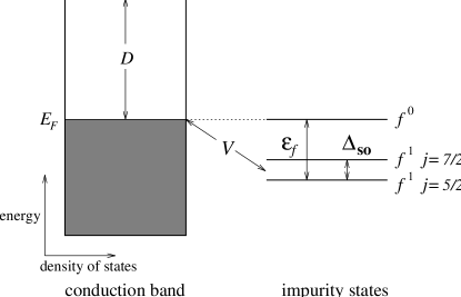
Refer to caption
FIG. 1.: Schematics of the $U=\infty$ single impurity Anderson model for Ce ions. $D$ is the conduction band width and $V$ is the single particle hybridization strength. The on site Coulomb interaction $U$ is infinity in our model.
Refer to caption
FIG. 2.: Schematic configuration diagram for the Uranium compound. $f^{2}$, $j=4$ and $f^{3}$, $j=9/2$ spin-orbit states are split by the crystal electric field. All the notations are explained in the text and all the values are listed in TableΒ II.
Refer to caption
FIG. 3.: Leading order Feynman diagrams for self energies. (a) pseudoboson self energy, $\Sigma_{0}(z)$r, (b) pseudo fermion($f^{1}$,$j$ multiplet) self energy $\Sigma_{jm}(z)$.
Refer to caption
FIG. 4.: Leading order Feynman diagram for static magnetic susceptibility. In this diagram, only $f$ electrons are coupled to the field.
Refer to caption
FIG. 5.: Feynman Diagram for the Knight shift calculation for Ce ions. This is the lowest order diagram of coupling between Ce local moment and nuclear spin in the infinite $U$ Anderson model. All the propagators are explained in the figure. For the incoherent calculation the conduction electron propagator is a bare electron propagator and when the the coherence effect for conduction electron is included ( multiple scattering off of $f$-sites) , it becomes a dressed propagator.
Refer to caption
FIG. 6.: Feynman Diagram for the additional contribution to the Knight shift which was noted by SΓΈrensen and Affleck [23, 24, 25]. This is significant in magnitude for distances beyond the Kondo screening cloud radius and not included in our calculation. This contribution is of potential importance for any dilute system, but is not important in our lattice calculation ( see, Sec.Β III D for discussion.). All the propagators are explained in the Fig.Β 5.
Refer to caption
FIG. 7.: Knight shift $K(r,T)$ at fixed angle $\theta=0$ and Kondo temperature $T_{0}=430K$ for Ce ions on a fine scale. We use the dimensionless variable $k_{F}r$ with the Fermi wave vector $k_{F}=0.65\AA^{-1}$ instead of $r$. Around $k_{F}r=3.2$ the lines of $T=104K$ and $T=52K$ are crossed. This can be explained that the Knight shift summation converges faster at higher temperatures and it has longer range at lower temperatures as mentioned by E.S. SΓΈrensen and I. Affleck [23, 24, 25].
Refer to caption
FIG. 8.: Knight shift $K(r,T)$ at fixed angle $\theta=0$ and Kondo temperature $T_{0}=430K$ for Ce ions. We use dimensionless variable $k_{F}r$ with the Fermi wave vector $k_{F}=0.65\AA^{-1}$ instead of $r$. This shows an oscillatory RKKY like behavior. The amplitude is decreased as the temperature is increased and the distance $r$ is increased. The calculations are done at the same temperatures in FigΒ 7.
Refer to caption
FIG. 9.: Knight shift $K(r,T)$ at fixed angle $\theta=\pi/2$ and Kondo temperature $T_{0}=430K$ for Ce ions on a fine scale. We use dimensionless variable $k_{F}r$ (with the Fermi wave vector $k_{F}=0.65\AA^{-1}$). The Knight shift has maximum amplitude around $T=104K$. Around $k_{F}r=2.8$ the lines of $T=174K$ and $T=52K$ are crossed.
Refer to caption
FIG. 10.: Knight shift $K(r,T)$ at fixed angle $\theta=\pi/2$ and Kondo temperature $T_{0}=430K$ for Ce ions. We use dimensionless variable $k_{F}r$ (with the Fermi wave vector $k_{F}=0.65\AA^{-1}$). This shows an oscillatory behavior like the RKKY interaction form and the amplitude is decreased as the temperature is increased and the distance $r$ is increased. The calculations are done at the temperatures in FigΒ 7.
Refer to caption
FIG. 11.: Calculated Knight shift $K(T)$ for a single Ce site vs. susceptibility $\chi(T)$ for varying separation with the Kondo scale used to fit the CeSn3 $\chi(T)$(see Fig.Β 13). For each plot the angle is held at $\theta=0$ with respect to the nuclear moment-Ce axis. The diagram of Fig.Β 5 is used to calculate $K(T)$. The magnitude of the non-linearity diminishes as $k_{F}r$ is reduced. The theoretical Knight shifts have been shifted by offset and scale factors to match the susceptibility; this does not affect the relative size of the anomaly.
Refer to caption
FIG. 12.: Calculated Knight shift $K(T)$ vs. susceptibility $\chi(T)$ for a single Ce site at $k_{F}r=3.33$ from a nuclear moment and angle $\Theta=0$. Fixing the $f$-level energy $\epsilon_{5/2}=-2$eV, and the spin orbit splitting Ξ”s​o=0.29​e​VsubscriptΞ”π‘ π‘œ0.29𝑒𝑉\Delta_{so}=0.29eV, the hybridization is varied to illustrate the dependence of the nonlinearity on the magnitude of $T_{0}$ (which ranges from 750 K to 130 K in these calculations as $\Gamma$ varies from $0.165eV$ to $0.130eV$). The diagram of Fig.Β 5 is used to calculate $K(T)$. The magnitude of the non-linearity diminishes as $T_{0}$ is reduced. The theoretical Knight shift has been shifted by a common offset and scale factor to match the susceptibility.
Refer to caption
FIG. 13.: Temperature dependence of 119Sn Knight Shift $K(T)$ and Ce $\chi(T)$ (both calculated and experimental results [5, 7]) for CeSn3. The theoretical $K(T)$ is calculated using the diagram of Fig.5 and with $T_{0}$ chosen to fit the experimental $\chi(T)$ data. A full (incoherent) lattice sum is carried out over several hundred shells of atoms.
Refer to caption
FIG. 14.: Temperature dependence of Knight Shift $K(T)$ with small constant damping $-\mbox{Im}\Sigma_{f}=0.01$ in incoherent lattice sum. In this figure $K(T)=\sum_{k_{F}r<k_{F}r_{0}}K(r,T)$. The calculations are done at the same temperatures in Fig.Β 7. The small absolute magnitude corresponds to the high temperature and it increases as the temperatures goes down. The convergence is slower than the coherence lattice sum.
Refer to caption
FIG. 15.: Temperature dependence of Knight Shift $K(T)$ with large constant damping $-\mbox{Im}\Sigma_{f}=1$ in incoherent lattice sum. In this figure $K(T)=\sum_{k_{F}r<k_{F}r_{0}}K(r,T)$. The calculations are done at the same temperatures in Fig.Β 7. The small absolute magnitude corresponds to the high temperature and it increases as the temperatures goes down. They converge very fast. an impurity at large distance doesn’t contribute to the total Knight shift because of the large damping, i.e. short life time of the conduction electrons.
Refer to caption
FIG. 16.: Temperature dependence of Knight Shift $K(T)$ with coherent lattice sum. In this figure $K(T)=\sum_{k_{F}r<k_{F}r_{0}}K(r,T)$. The calculations are done at the same temperatures in Fig.Β 7. The small absolute magnitude corresponds to the high temperature and it increases as the temperatures goes down. The convergence is faster than the small damping case but slower than larger damping case.
Refer to caption
FIG. 17.: Temperature dependence of 119Sn Knight Shift $K(T)$ with coherence effect and Ce $\chi(T)$ (both calculated and experimental results [5, 7]) for CeSn3. The theoretical $K(T)$ is calculated using the diagram of Fig.Β 5 and with $T_{0}$ chosen to fit the experimental $\chi(T)$ data. A full coherent lattice sum is carried out over several hundred shells of atoms using the average T-matrix approximation to approximate the coherent conduction self energy.
Refer to caption
FIG. 18.: Temperature dependence of positive muon Knight Shift $K(T)$ and Ce $\chi(T)$ (both calculated and experimental results [7, 56]) for CeSn3. The theoretical $K(T)$ is calculated assuming that muon sits at the center of cubic unit cell. Other parameters are same as for the 119Sn NMR Knight shift calculation.
Refer to caption
FIG. 19.: Temperature dependence of positive muon Knight Shift $K(T)$ and Ce $\chi(T)$ (both calculated and experimental results [7, 56]) for CeSn3. The theoretical $K(T)$ is calculated assuming that muon sits at the middle of the axis between the Ce atoms. Other parameters are same as for the 119Sn NMR Knight shift calculation.
Refer to caption
FIG. 20.: Temperature dependence of positive muon Knight Shift $K(T)$ and Ce $\chi(T)$ (both calculated and experimental results [7, 56]) for CeSn3. The theoretical $K(T)$ is calculated averaging the $\mu$sr Knight shift from both positions with fractional occupancy ratio $f=2/3$ ( 2/3 of the muon is at the center of CeSn3 unit cell.).
Refer to caption
FIG. 21.: Temperature dependence of 27Al Knight Shift $K(T)$ and Yb $\chi(T)$ (both calculated and experimental resultsΒ [6, 7, 61]) for YbCuAl. The theoretical $K(T)$ is calculated using the diagram of Fig.Β 5 and with $T_{0}$ chosen to fit the experimental $\chi(T)$ data. A full (incoherent) lattice sum is carried out over twenty four thousand atoms.
Refer to caption
FIG. 22.: Temperature dependence of 89Y Knight Shift $K(T)$ and U $\chi(T)$ (both calculated and experimental resultsΒ [10, 67]) for Y0.8U0.2Pd3. The theoretical $K(T)$ is calculated using the diagram of Fig.Β 5 and with $T_{0}$ chosen to fit the experimental $\chi(T)$ data. A full (incoherent) lattice sum and impurity configuration averaging is carried out over a several shells.
TABLE I.: Ground states and parameter values for, Ce and Yb ions model. $j_{g}$ is the ground state spin- orbit multiplet angular momentum and $j_{ex}$ is the excited state multiplet angular momentum. $N_{g}(N_{ex})$ is the degeneracy of the ground (first excited) state multiplet. $\epsilon_{f}$ is the energy of the ground configuration. and Ξ”s​osubscriptΞ”π‘ π‘œ\Delta_{so} is the energy difference between the $j_{g}$ and $j_{ex}$ multiplets
Ce Yb
Β Β Β Β Β Β Β Β Β β€…Configuration $4f^{1}$ $4f^{13}$
$4f^{0}$ $4f^{14}$
Β Β Β Β Β Β Β Β Β β€…jgsubscript𝑗𝑔j_{g} 5/2 7/2
Β Β Β Β Β Β Β Β Β β€…je​xsubscript𝑗𝑒π‘₯j_{ex} 7/2 5/2
Β Β Β Β Β Β Β Β Β β€…Ngsubscript𝑁𝑔N_{g} 6 8
Β Β Β Β Β Β Β Β Β β€…Ne​xsubscript𝑁𝑒π‘₯N_{ex} 8 6
Β Β Β Β Β Β Β Β Β β€…Ο΅fsubscriptitalic-ϡ𝑓\epsilon_{f} $-2eV$ $-1eV$
Β Β Β Β Β Β Β Β Β β€…Ξ”s​osubscriptΞ”π‘ π‘œ\Delta_{so} $0.29eV$ $1.3eV$
TABLE II.: Parameter values for Y0.8U0.2Pd3 in units of the conduction electron band width $D=3eV$. $\epsilon_{f}$ is the energy of $j=4$ multiplet and $\Delta_{ij}$ is the energy difference between crystal field split $\Gamma_{i}$ and $\Gamma_{j}$ states. $\Gamma$ is the single impurity hybridization width. For the definition of $x$ and $W$, see AppendixΒ B. $x_{2}$ and $W_{2}$ are for $f^{2}$ configuration and $x_{3}$ and $W_{3}$ are for $f^{3}$ configuration.
Β Β Β Β Β Β Β Β Β Β Β Β Β β€…Ο΅fsubscriptitalic-ϡ𝑓\epsilon_{f} -0.333
Β Β Β Β Β Β Β Β Β Β Β Β Β β€…Ξ”35subscriptΞ”35\Delta_{35} 0.003
Β Β Β Β Β Β Β Β Β Β Β Β Β β€…Ξ”34subscriptΞ”34\Delta_{34} 0.008175
Β Β Β Β Β Β Β Β Β Β Β Β Β β€…Ξ”31subscriptΞ”31\Delta_{31} 0.019621
Β Β Β Β Β Β Β Β Β Β Β Β Β β€…Ξ”68​asubscriptΞ”68π‘Ž\Delta_{68a} 0.000136
Β Β Β Β Β Β Β Β Β Β Β Β Β β€…Ξ”68​bsubscriptΞ”68𝑏\Delta_{68b} 0.013190
              $\Gamma$ 0.15
Β Β Β Β Β Β Β Β Β Β Β Β Β β€…x2subscriptπ‘₯2x_{2} -0.648
Β Β Β Β Β Β Β Β Β Β Β Β Β β€…W2subscriptπ‘Š2W_{2} $-3.95\times 10^{-4}$
Β Β Β Β Β Β Β Β Β Β Β Β Β β€…x3subscriptπ‘₯3x_{3} 0.3693
Β Β Β Β Β Β Β Β Β Β Β Β Β β€…W3subscriptπ‘Š3W_{3} $2.746\times 10^{-4}$
TABLE III.: Explicit values of both incoherent and coherent Knight shift at high temperatures. They have similar values because coherent lattice effects are small at high temperatures. These are unadjusted data.
Β Β Β Β Β Β Β β€…Temperature Knight Shift
Incoherent Coherent
Β Β Β Β Β Β Β β€…925K -0.3579 -0.44855
Β Β Β Β Β Β Β β€…615K -2.4078 -2.42525
Β Β Β Β Β Β Β β€…555K -3.0157 -2.84562
Β Β Β Β Β Β Β β€…490K -3.7184 -3.34231
Β Β Β Β Β Β Β β€…430 -4.5380 -3.95714
TABLE IV.: Crystal electric field energy eigenstates for $j=4$ multiplet in the cubic symmetry. The coefficient is independent of x
Β Β Β Β Β Β Β Β Β β€…j=4𝑗4j=4 multiplet states
Β Β Β Β Β Β Β Β Β β€…|Ξ“1⟩ketsubscriptΞ“1|\Gamma_{1}\rangle $\sqrt{\frac{5}{24}}|4\rangle+\sqrt{\frac{7}{12}}|0\rangle+\sqrt{\frac{5}{24}}|-4\rangle$
Β Β Β Β Β Β Β Β Β β€…|Ξ“3;+⟩ketsubscriptΞ“3|\Gamma_{3};+\rangle $\frac{1}{\sqrt{2}}(|2\rangle+|-2\rangle)$
Β Β Β Β Β Β Β Β Β β€…|Ξ“3;βˆ’βŸ©ketsubscriptΞ“3|\Gamma_{3};-\rangle $-\sqrt{\frac{5}{24}}|4\rangle+\sqrt{\frac{7}{12}}|0\rangle-\sqrt{\frac{5}{24}}|-4\rangle$
Β Β Β Β Β Β Β Β Β β€…|Ξ“4;0⟩ketsubscriptΞ“40|\Gamma_{4};0\rangle $\frac{1}{\sqrt{2}}(|4\rangle-|-4\rangle)$
Β Β Β Β Β Β Β Β Β β€…|Ξ“4;Β±1⟩ketsubscriptΞ“4plus-or-minus1|\Gamma_{4};\pm 1\rangle $\frac{1}{\sqrt{8}}|\mp 3\rangle+\sqrt{\frac{7}{8}}|\pm 1\rangle$
Β Β Β Β Β Β Β Β Β β€…|Ξ“5;0⟩ketsubscriptΞ“50|\Gamma_{5};0\rangle $\frac{1}{\sqrt{2}}(|2\rangle-|-2\rangle)$
Β Β Β Β Β Β Β Β Β β€…|Ξ“5;Β±1⟩ketsubscriptΞ“5plus-or-minus1|\Gamma_{5};\pm 1\rangle $\frac{1}{\sqrt{8}}|\mp 3\rangle-\sqrt{\frac{7}{8}}|\pm 1\rangle$
TABLE V.: Crystal electric field energy eigenstate for $j=9/2$ multiplet in the cubic symmetry, the coefficient $a_{i}$’s and $b_{j}$’s depend on the $x$ which is the parameter which depends on the ratio of the fourth and sixth degree cubic field in the Hamiltonian of the crystal electric field. In this calculation, we use $x_{3}=0.3693$ and $W_{3}=2.746\times 10^{-4}$ to have $j=9/2$ $\Gamma_{6}$ for the ground state of the $f^{3}$ configuration and $x_{2}=-0.648$ and $W_{2}=-3.95\times 10^{-4}$ to have $j=4$ $\Gamma_{3}$ for the ground state for $f^{2}$ configuration.
Β Β Β Β Β β€…j=9/2𝑗92j=9/2 multiplet states
Β Β Β Β Β β€…|Ξ“6;±⟩ketsubscriptΞ“6plus-or-minus|\Gamma_{6};\pm\rangle $\sqrt{\frac{9}{24}}|\pm\frac{9}{2}\rangle+\sqrt{\frac{1}{24}}|\mp\frac{7}{2}\rangle+\sqrt{\frac{7}{12}}|\pm\frac{1}{2}\rangle$
Β Β Β Β Β β€…|Ξ“8​a;1,±⟩ketsubscriptΞ“8π‘Ž1plus-or-minus|\Gamma_{8a};1,\pm\rangle $a_{1}\leavevmode\leavevmode\hbox{${}^{\rm a}$}|\pm\frac{9}{2}\rangle+a_{2}|\mp\frac{7}{2}\rangle+a_{3}|\pm\frac{1}{2}\rangle)$
Β Β Β Β Β β€…|Ξ“8​a;2,±⟩ketsubscriptΞ“8π‘Ž2plus-or-minus|\Gamma_{8a};2,\pm\rangle $b_{1}|\pm\frac{5}{2}\rangle+b_{2}|\mp\frac{3}{2}\rangle$
Β Β Β Β Β β€…|Ξ“8​b;1,±⟩ketsubscriptΞ“8𝑏1plus-or-minus|\Gamma_{8b};1,\pm\rangle $a_{6}|\pm\frac{9}{2}\rangle+a_{7}|\mp\frac{7}{2}\rangle+a_{8}|\pm\frac{1}{2}\rangle)$
Β Β Β Β Β β€…|Ξ“8​b;2,±⟩ketsubscriptΞ“8𝑏2plus-or-minus|\Gamma_{8b};2,\pm\rangle $b_{3}|\pm\frac{5}{2}\rangle+b_{4}|\mp\frac{3}{2}\rangle$
TABLE VI.: Crystal electric field energy eigenstates for $j=5/2$ multiplet in the cubic symmetry.
Β Β Β Β Β Β Β β€…j=5/2𝑗52j=5/2 Multiplet States
Β Β Β Β Β Β Β β€…|Ξ“7(5/2);↑/β†“βŸ©|\Gamma_{7}^{(5/2)};\uparrow/\downarrow\rangle $-\sqrt{1\over 6}~{}|\pm 5/2\rangle+\sqrt{5\over 6}~{}|\mp 3/2\rangle$
Β Β Β Β Β Β Β β€…|Ξ“8(5/2);+,↑/β†“βŸ©|\Gamma_{8}^{(5/2)};+,\uparrow/\downarrow\rangle $|\pm 1/2\rangle$
Β Β Β Β Β Β Β β€…|Ξ“8(5/2);βˆ’,↑/β†“βŸ©|\Gamma_{8}^{(5/2)};-,\uparrow/\downarrow\rangle $\sqrt{5\over 6}~{}|\pm 5/2\rangle+\sqrt{1\over 6}~{}|\mp 3/2\rangle$
TABLE VII.: Crystal electric field energy eigenstates for $j=7/2$ multiplet in the cubic symmetry.
Β Β Β Β Β Β Β β€…j=7/2𝑗72j=7/2 Multiplet States
Β Β Β Β Β Β Β β€…|Ξ“6(7/2);↑/β†“βŸ©|\Gamma_{6}^{(7/2)};\uparrow/\downarrow\rangle $\pm\sqrt{5\over 12}~{}|\mp 7/2\rangle\pm\sqrt{7\over 12}~{}|\pm 1/2\rangle$
Β Β Β Β Β Β Β β€…|Ξ“7(7/2);↑/β†“βŸ©|\Gamma_{7}^{(7/2)};\uparrow/\downarrow\rangle $\pm{\sqrt{3}\over 2}~{}|\pm 5/2\rangle\mp{1\over 2}~{}|\mp 3/2\rangle$
Β Β Β Β Β Β Β β€…|Ξ“8(7/2);+,↑/β†“βŸ©|\Gamma_{8}^{(7/2)};+,\uparrow/\downarrow\rangle $\pm\sqrt{7\over 12}~{}|\mp 7/2\rangle\mp\sqrt{5\over 12}~{}|\pm 1/2\rangle$
Β Β Β Β Β Β Β β€…|Ξ“8(7/2);βˆ’,↑/β†“βŸ©|\Gamma_{8}^{(7/2)};-,\uparrow/\downarrow\rangle $\pm{1\over 2}~{}|\pm 5/2\rangle\pm{\sqrt{3}\over 2}~{}|\mp 3/2\rangle$
TABLE VIII.: Selection rules for the Anderson hybridization between $f^{2}$ $\Gamma$ and $f^{3}$ $\Gamma$ CEF states. The meaning, for example, is that a $\Gamma_{6}$ conduction electron doublet can combine with the $f_{2}$ $\Gamma_{3}$ doublet to make an $f^{3}$ $\Gamma_{8}$ quartet.
Β Β Β Β Β Β Β Β Β Β Β Β Β β€…Ξ“cβŠ—f2​Γtensor-productsubscriptΓ𝑐superscript𝑓2Ξ“\Gamma_{c}\otimes f^{2}\Gamma $f^{3}\Gamma$ CEF states
Β Β Β Β Β Β Β Β Β Β Β Β Β β€…Ξ“cβŠ—Ξ“1tensor-productsubscriptΓ𝑐subscriptΞ“1\Gamma_{c}\otimes\Gamma_{1} $\Gamma_{c}$
Β Β Β Β Β Β Β Β Β Β Β Β Β β€…Ξ“6βŠ—Ξ“3tensor-productsubscriptΞ“6subscriptΞ“3\Gamma_{6}\otimes\Gamma_{3} $\Gamma_{8}$
Β Β Β Β Β Β Β Β Β Β Β Β Β β€…Ξ“7βŠ—Ξ“3tensor-productsubscriptΞ“7subscriptΞ“3\Gamma_{7}\otimes\Gamma_{3} $\Gamma_{8}$
Β Β Β Β Β Β Β Β Β Β Β Β Β β€…Ξ“8βŠ—Ξ“3tensor-productsubscriptΞ“8subscriptΞ“3\Gamma_{8}\otimes\Gamma_{3} $\Gamma_{6}\oplus\Gamma_{7}\oplus\Gamma_{8}$
Β Β Β Β Β Β Β Β Β Β Β Β Β β€…Ξ“6βŠ—Ξ“4tensor-productsubscriptΞ“6subscriptΞ“4\Gamma_{6}\otimes\Gamma_{4} $\Gamma_{6}\oplus\Gamma_{8}$
Β Β Β Β Β Β Β Β Β Β Β Β Β β€…Ξ“7βŠ—Ξ“4tensor-productsubscriptΞ“7subscriptΞ“4\Gamma_{7}\otimes\Gamma_{4} $\Gamma_{7}\oplus\Gamma_{8}$
Β Β Β Β Β Β Β Β Β Β Β Β Β β€…Ξ“8βŠ—Ξ“4tensor-productsubscriptΞ“8subscriptΞ“4\Gamma_{8}\otimes\Gamma_{4} $\Gamma_{6}\oplus\Gamma_{7}\oplus 2\Gamma_{8}$
Β Β Β Β Β Β Β Β Β Β Β Β Β β€…Ξ“6βŠ—Ξ“5tensor-productsubscriptΞ“6subscriptΞ“5\Gamma_{6}\otimes\Gamma_{5} $\Gamma_{7}\oplus\Gamma_{8}$
Β Β Β Β Β Β Β Β Β Β Β Β Β β€…Ξ“7βŠ—Ξ“5tensor-productsubscriptΞ“7subscriptΞ“5\Gamma_{7}\otimes\Gamma_{5} $\Gamma_{6}\oplus\Gamma_{8}$
Β Β Β Β Β Β Β Β Β Β Β Β Β β€…Ξ“8βŠ—Ξ“5tensor-productsubscriptΞ“8subscriptΞ“5\Gamma_{8}\otimes\Gamma_{5} $\Gamma_{6}\oplus\Gamma_{7}\oplus 2\Gamma_{8}$