Orbital Kondo-effect from tunneling impurities

Abstract

The article reviews recent results for the low energy physics of fast tunneling centers in metallic environments. For strong enough couplings to the environment these tunneling centers display an orbital Kondo effect and give rise to a non-Fermi-liquid behavior. This latter property is explained by establishing a mapping of the tunneling center model to the multichannel Kondo model via the renormalization group transformation combined with a $1/N_{f}$ expansion. The case of $M$-state systems, the role of the splittings and the present experimental situation are also discussed.

I Introduction

Non-Fermi-liquid systems like some heavy fermion materials,[1] one-dimensional interacting electrons[2] or multichannel quantum impurity problems [3, 4] have been the subject of growing interest during the past few years. These systems have the common feature that they display nonanalytical power law singularities in various physical properties and that the usual quasiparticle picture of Landau’s Fermi-liquid theory [5, 6] does not apply for them.

From the systems mentioned above quantum impurity problems are of special interest. This is due to the fact that they provide simple toy models for the study of strongly correlated lattice models and furthermore the techniques developed for them can be directly applied to finite [7, 8] and infinite dimensional lattice models.[9] These latters seem to be very close to the realistic two or three-dimensional models designed to describe heavy fermion compounds.[10] Furthermore it has been suggested that even the properties of high-$T_{c}$ materials might be explained by means of multichannel Kondo-like models.[11]

One of the most interesting quantum impurity problems is provided by tunneling centers (TC). These are formed by some heavy particle (an atom, a point defect or a collective coordinate of a dislocation) moving in an effective potential with at least two local minima. If the barrier between these minima is sufficiently large and the minima are close enough to each other then at low temperature the hopping via thermal activation is negligible and the atom can move only by tunneling from one minimum to another. At low enough temperatures the heavy particle stays in the lowest lying quantum states associated to the minima of the effective potential and the presence of the higher excited states is only reflected in the renormalization of the different coupling constants characterizing the interaction of the TC with its surrounding (See Sec. VII B).

The physics of an isolated TC is rather boring, but becomes interesting if the TLS is coupled to its environment. In this paper we restrict our considerations to TC’s put into a metal. A realistic TC in a metal is coupled both to the acoustic phonons and the conduction electrons providing the low energy excitations of the environment. However, as also stressed by Prokof’ev,[12] since the phonon-TC coupling is proportional to the momentum transfer $q$ and the density of the low-energy phonon modes scales as $\sim\omega^{2}$ this interaction can be neglected with respect to the coupling to the low energy electron-hole excitations, which have a linear density of states and an energy independent coupling to the TC.

The TC is coupled to the conduction electrons by two different processes.[13, 14] For a fixed position of the heavy particle the conduction electrons tend to build up a screening cloud around the tunneling particle. Since by a tunneling process the heavy particle has to carry with itself this screening cloud consisting of an infinite number of electron-hole excitations, this interaction tends to localize the heavy particle reducing its tunneling rate at low temperatures. For slow tunneling centers displaying individual jumps this is the only important process and it has been studied in great detail both experimentally and theoretically.[15, 16, 17] If only this screening interaction is taken into account then the different vertices occurring in a perturbative expansion commute with each other. Therefore this model is sometimes also referred to as the commutative model.

On the other hand, if the tunneling rate is large enough, then in addition to the screening electron assisted tunneling becomes also possible (noncommutative model).[13, 18] In this process an electron is scattered on the heavy particle while it jumps from one minimum to another. The latter is essentially due to barrier fluctuations caused by the local electronic density fluctuations [18, 19] but it can also be generated by the virtual hoppings to the excited states of the TC.[20] While the amplitude of this process is rather small, it results in the generation of a Kondo effect and drives the system away from the marginally stable commutative model at low energy scales. As the temperature decreases, the conduction electrons and the heavy particle form a strongly correlated Kondo-like bound state.[14, 18, 21] For a two-level system (TLS), the important case of a TC with two potential minima, the energy of this ground state is approximately given by the Kondo energy

$$T_{K}^{\rm orb}=D(v^{x}v^{z})^{1/2}\left({v^{x}\over 4v^{z}}\right)^{1/4v^{z}}\;,$$ (1)

where $D$ is some bandwidth cutoff of the order of the Fermi energy, and $v^{z}$ and $v^{x}$ denote the dimensionless couplings characteristic to screening and assisted tunneling, respectively. For an $M$-level system no such simple formula can be given, but the estimated maximal Kondo temperatures are of the same order of magnitude, $T_{K}^{\rm orb}\sim 1{\rm K}$.[21]

In the considerations of the previous paragraph we have neglected the role of the splitting $\Delta$ of the nearly degenerate levels of the TC. While this splitting is usually small and it is also renormalized downward during the scaling procedure it generates a further low energy scale called the freezing temperature $T^{\ast}$. Above this scale the levels of the TC can be considered as degenerate. On the other hand, below $T^{*}$ the splitting becomes relevant and the internal degrees of freedom leading to the Kondo effect are in most cases frozen out.[58]

Usually one assumes that the interaction of heavy particle and the conduction electrons is independent of the spin of the electrons, thus the spin up and spin down conduction electron channels are scattered independently and exactly with the same amplitude by the heavy particle. While the spin is only present as a silent quantum number (flavor) it plays a crucial role. As discussed later, in the appropriate temperature range $T^{*}<T<T_{K}$ the low energy properties of an $M$-state TC can be described by the two channel $SU(M)\times SU(N_{f}=2)$ Coqblin-Schrieffer model, [18, 21, 22, 23] a *** generalization of the multichannel Kondo model. Here the $SU(M)$ symmetry is connected to the $M$ positions of the TC, while the $SU(2)$ symmetry is due to the spins of the conduction electrons. This model, in contrast to the usual $SU(M)$ single channel model exhibiting a Fermi-liquid behavior,[3, 29, 30] belongs to the family of overcompensated spin models and displays non-Fermi-liquid properties due to the $N_{f}$-fold degeneracy in the ’flavor’, and gives rise to nonanalytical behavior of the different physical quantities.[21, 31, 32, 33] In the special case of a TLS ($M=2$) the equivalent model is just the two-channel Kondo model. While the usual $SU(2)\times SU(2)$ two-channel Kondo model has been investigated by various techniques such as Bethe Ansatz, [49, 50, 51] conformal field theory,[24] large $N$ expansions,[8] numerical renormalization group,[25] path integral approach,[26, 27] and bosonazitaions,[28] the number of results obtained for the $SU(M)\times SU(N)$ model with $M\geq 3$ is still more restrictive.

In the present review we mainly concentrate on the mapping of the noncommutative TC model to the $SU(M)\times SU(N)$ model in the above described temperature range, but we also give a concise review of the recent experimental and theoretical results in the field.

The paper is organized as follows: In Section II we shortly discuss the model introduced to describe a tunneling heavy particle. In Sec. III we discuss the origin of the logarithmic corrections appearing in the perturbation theory and apply Anderson’s ’poor man’s scaling’ to the TLS problem.[34] Then in Sec. IV we give a concise introduction to the multiplicative renormalization group and we show how to obtain the estimation of the Kondo temperature (1). Section V is devoted to the development of a large $N_{f}$ expansion in the ’flavor degeneracy’, $N_{f}$ for the TLS. We show that up to $1/N_{f}^{2}$ order the generalized $N_{f}$-flavor TLS model can be mapped to the $N_{f}$-channel Kondo model. The generalization of the above mapping to the case of $M$-state systems will be discussed in Sec. VI. Some additional results not closely connected to the subject of this paper such as the path integral formalism applied to two-level systems, the influence of spin-flip scattering on the TLS, and the role of excited states will be shortly discussed in Sec. VII. We also discuss the present experimental situation and the possibility of the observation of the non-Fermi-liquid behavior, predicted in Sec. VIII. Finally, our concluding remarks are given in Section IX.

II The two-state model

To investigate the behavior of two-level system (TLS) coupled to the conduction electrons we first have to construct a model that contains all the relevant ingredients of the realistic situation. In the present Section we restrict our considerations to the case of TLSs but they can easily be extended to the general case of M-level systems (MLSs).

In the nature a variety of physical realizations of TLS’s exist. However, to be specific, constructing the model we consider the case of amorphous metals being one of the most frequently studied systems containing TLSs.[35] The construction of the model for other systems follows similar lines. In Fig 1.a we represent a situation when one or several neighboring atoms (ions) in the amorphous structure have two stabile positions close to each-other. This situation can be most easily described by some effective potential shown in Fig. 1.b, where $R$ denotes the relevant variable in the configuration space [15] and the two minima are associated to the two positions of the TLS in Fig. 1.a. Then one can associate two quantum states $\phi_{l}(R)$ and $\phi_{r}(R)$ of the atoms to the two minima of the potential well, which are localized in the left- and right-hand side, respectively. We assume, that the shape of the double well potential is such that there are two low-energy states with energies $E_{1}\approx E_{2}$: two linear combinations of $\phi_{l}(R)$ and $\phi_{r}(R)$, and the next one has a much higher energy: $E_{3}-E_{1}\sim\omega_{\rm Debye}$. With this assumption the motion of the TLS at low temperatures will be constrained to the two lowest lying states and therefore the states having higher energies can be ignored. In an amorphous metal the energy distance $\Delta$ between the two lowest states can differ from TLS to TLS.

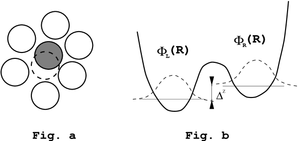
FIG. 1.: The TLS in an amorphous structure and the effective potential describing its motion.

In the following considerations we restrict ourselves to a single TLS and an electron band of the simplest shape. To obtain macroscopic quantities we shall treat each TLS as being independent of the other TLS’s and in the end of the calculation we perform an averaging over the distribution of the individual TLS parameters. The separation of this last summation is reliable at low TLS concentration, i.e., when they are far from one another and do not interact.

At low enough temperatures the Hamiltonian for a TLS could be described simply by a $2\times 2$ matrix acting in the space of the states $\phi_{l}(R)$ and $\phi_{r}(R)$. Nevertheless, for later convenience we rather describe the TLS motion in terms of an imaginary fermion (pseudofermion), initially introduced by Abrikosov [36] to make the second quantized formalism applicable for the Kondo problem. In this language the physical states $\phi_{l}(R)$ and $\phi_{r}(R)$ of the TLS correspond to the one particle pseudofermion states $b^{+}_{l}|0\rangle$ and $b^{+}_{r}|0\rangle$, respectively, $b^{+}_{l}$ and $b^{+}_{r}$ being the pseudofermion creation operators. The nonphysical zero pseudofermion state $|0\rangle$ gives no contribution to the electron scattering, while the two pseudofermion state $b^{+}_{l}b^{+}_{r}|0\rangle$ can be projected out by making it thermodynamically very improbable. This latter can be achieved if we choose the pseudofermion chemical potential $\lambda$ to be very high $\lambda\to\infty$. In this limit the leading terms to any physical quantity will be dominated by the one pseudofermion states and the two-fermion contributions will be suppressed by a factor $\sim e^{-\beta\lambda}$ with respect to them. Physical quantities must be normalized to the number of pseudofermions present, $2e^{-\beta\lambda}$.

The general form of a TLS Hamiltonian can be written as:

$$H_{\rm TLS}=\lambda\sum_{\alpha}b^{+}_{\alpha}b_{\alpha}+\sum_{i,\alpha,\alpha^{\prime}}\Delta^{i}b^{+}_{\alpha}\tau^{i}_{\alpha\alpha^{\prime}}b_{\alpha^{\prime}}\;,$$ (2)

the Pauli matrices $\tau^{i}_{\alpha\alpha^{\prime}}$ ($i=x,y,z$) denote the ’pseudospin’ of the TLS and $\alpha=l,r$ labels the states of the TLS. The coefficient $\Delta^{z}$ describes the asymmetry energy between the left- and right sides of the TLS while $\Delta^{x}$ and $\Delta^{y}$ stand for the tunneling transition (see Fig 1). The splitting of the lowest-lying two states of the TLS can be expressed via these quantities as $\Delta=2(\sum_{i}\Delta_{i}^{2})^{1/2}$.

As we shall see, only electrons close to the Fermi surface interact effectively with the TLS. Therefore, in the spirit of Landau’s Fermi-liquid theory [5] the conduction electrons are treated as noninteracting ones and their Hamiltonian is written as

$$H_{e}=\sum_{\epsilon,n,s}\epsilon a^{+}_{\epsilon ns}a_{\epsilon ns}\;,$$ (3)

where $a^{+}_{\epsilon ns}$ and $a_{\epsilon ns}$ are the electrons’ creation and annihilation operators with spin $s$ and energy $\epsilon$. The quantum number $n$ classifies the orbital structure of the states. It can be, e.g., a spherical wave index-pair $n=(l,m)$ in the free electron case, or a crystal field index reflecting the symmetry of the host.

In our calculations we mostly use a simplified density of states for the electrons,

$$\varrho(\epsilon)=\cases{\varrho_{0}&if $-D<\epsilon<D$,\cr 0&otherwise,}$$ (4)

where we assumed that the band can be characterized practically by only two parameters: the density of states at the Fermi level $\varrho_{0}$ and the band width $D$. The role of the energy dependence of the density of states will be discussed in Sec. VII.

The most general form of the interaction between the electrons and the TLS can be written as

$$H_{i}=\sum_{\textstyle{\epsilon,n,\epsilon^{\prime},n^{\prime},s\atop\mu,\alpha,\alpha^{\prime}}}a^{+}_{\epsilon ns}b^{+}_{\alpha}V^{\mu}_{nn^{\prime}}\tau^{\mu}_{\alpha\alpha^{\prime}}b_{\alpha^{\prime}}a_{\epsilon^{\prime}n^{\prime}s}\;,$$ (5)

where $\mu={0},x,y,z$ and $\tau^{0}_{\alpha\alpha^{\prime}}=\delta_{\alpha\alpha^{\prime}}$. In the following we use the convention that Greek indices, $\mu,\nu,..$, take the values $\{0,x,y,z\}$, while the Roman letters, $i,j,..$,will only be used for the components $x,y,z$. Note that in Eq. (5) the couplings $V^{\mu}_{nn^{\prime}}$ are assumed to be energy-independent. This assumption usually does not influence the infra-read behavior of logarithmically divergent models. The real electron spin $s$ plays the silent role of flavor, i.e., the couplings do not depend on it, but its multiplicity will essentially affect the ground state and the low temperature behavior of the system.

Assuming a simple two-body interaction between the TLS and the conduction electrons the coupling constants in Eq. (5) can be estimated by simple integrals.[18, 19] The physical interpretation of these coupling constants is as follows. $V^{0}\pm V^{z}$ describe the on site electron scattering on the two positions of the TLS. If the moving particle is an ion different from the host, then this part of the interaction may be strong, $\varrho_{0}V^{0}\pm\varrho_{0}V^{z}\sim 1$. These couplings are responsible for the generation of the Friedel-oscillations. The coupling $V^{z}$, also sometimes called the ’screening interaction’, describes the fact that the electrons are scattered differently if the TLS is sitting in its left- and right position, and if the distance $d$ between the two sites is small, $k_{F}d\ll 1$, then $V^{z}\ll V^{0}$. It is the coupling $V^{z}$ which is responsible for the eventual localization of the TLS discussed in the Introduction.

The terms proportional to $V^{x}\pm iV^{y}$ describe electron assisted tunneling of the heavy particle between the two TLS sites, i.e. processes where a conduction electron is scattered by the TLS flipping from one side to the other simultaneously. These processes are graphically depicted in Fig. 2. They are mostly generated by the fluctuations of the barrier of the TLS potential due to the local electronic charge fluctuations.[18, 19] Since they contain the overlap integral between the heavy particle states $\phi_{l}(R)$ and $\phi_{r}(R)$, they are much smaller then the on site terms: $V^{x}\pm iV^{y}\ll V^{z}$.[18]

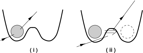
FIG. 2.: Sketch of the screening interaction (i) and the assisted tunneling process (ii).

III Logarithmic corrections in leading order and orbital Kondo effect

Having established our microscopic model we turn to the analysis of the perturbation series. We use the Matsubara-technique to handle the interacting electron-pseudofermion system. The following imaginary time Green’s functions are introduced for the two types of particles:[5]

$$G_{e}(\epsilon,n,\tau,\epsilon^{\prime},n^{\prime},\tau^{\prime})=-\bigl{\langle}\mathop{{\rm T}_{\tau}}\nolimits\bigl{[}a_{\epsilon ns}(\tau)a^{+}_{\epsilon^{\prime}n^{\prime}s}(\tau^{\prime})\bigr{]}\bigr{\rangle}\;,$$ (6)

$${\cal G}(\alpha,\tau,\alpha^{\prime},\tau^{\prime})=-\bigl{\langle}\mathop{{\rm T}_{\tau}}\nolimits\bigl{[}b_{\alpha}(\tau)b^{+}_{\alpha^{\prime}}(\tau^{\prime})\bigr{]}\bigr{\rangle}\;.$$ (7)

Here $\mathop{{\rm T}_{\tau}}\nolimits$ is the $\tau$-ordering operator, the operators $a_{\epsilon ns}(\tau)$ and $b_{\alpha}(\tau)$ are in Heisenberg representation and the angular brackets denote thermodynamic average. Then the unperturbed Green’s functions in Fourier representation are given by

$$G_{e}^{0}(\omega)=\bigl{(}\omega-\epsilon\bigr{)}^{-1}\;,$$ (8)

$${\cal G}^{0}(\omega)={\textstyle\bigl{(}\omega-\Delta^{i}\tau^{i}\bigr{)}}^{-1}\;,$$ (9)

where $\omega$ denotes a Matsubara frequency $\omega=i\omega_{n}$ and the pseudofermion frequency has been measured from the chemical potential $\lambda$. In Eq. (9) a short matrix notation was used for $G_{e}$ and ${\cal G}$ whose indices $\epsilon n$ and $\alpha$ have been suppressed, respectively.

As in the case of the Kondo effect, the perturbation theories lead to logarithmically divergent contributions to different quantities as the relevant energy scale or the temperature tends to zero. To demonstrate this we calculate the vertex corrections of the lowest order depicted in Fig. 3, where the solid lines stand for the electrons and the dotted lines stand for the pseudofermions. Their contribution is

$$\int_{-D}^{+D}\varrho_{0}\,d\epsilon\sum_{i,j,n_{1},\alpha_{1},\alpha_{2}}\biggl{(}V^{i}_{nn_{1}}V^{j}_{n_{1}n^{\prime}}\tau^{i}_{\alpha\alpha_{1}}\left({1-n(\epsilon)\over\omega-\epsilon-\Delta^{i}\tau^{i}}\right)_{\alpha_{1}\alpha_{2}}\tau^{j}_{\alpha_{2}\alpha^{\prime}}$$ (10)

$$\hskip 84.0pt-V^{j}_{nn_{1}}V^{i}_{n_{1}n^{\prime}}\tau^{i}_{\alpha\alpha_{1}}\left({n(\epsilon)\over\omega+\epsilon-\Delta^{i}\tau^{i}}\right)_{\alpha_{1}\alpha_{2}}\tau^{j}_{\alpha_{2}\alpha^{\prime}}\biggr{)}\;,$$ (11)

where $\omega$ is the initial energy of the incoming electron, $\varrho_{0}$ denotes the density of states at the fermi energy, and $n(\epsilon)$ is the Fermi distribution function at temperature $T$. (For the sake of simplicity we put the pseudofermion energy at the chemical potential $\lambda$: $\omega_{\rm ps}=0$.)

FIG. 3.: Lowest order vertex corrections in the perturbation theory.

The energy integral can be approximated by $\ln(D/\max\{|\omega|,T,\Delta\})$, where $\Delta=\bigl{(}\sum_{i}{\Delta^{i}}^{2}\bigr{)}^{1/2}$, and terms of the order of unity have been neglected with respect to the logarithm. For the sake of simplicity we will consider the case when $|\omega|$ is the largest energy scale. (The case $T>\Delta,|\omega|$ can be treated similarly while the discussion of the case $\Delta>T,|\omega|$ will be posponed to Sec. IV.) Then the vertex in the first order approximation (11) gets the form:

$$\underline{\Gamma}^{i}(\omega)={\underline{V}}^{i}-2i\varepsilon^{ijk}\varrho_{0}{\underline{V}}^{j}{\underline{V}}^{k}\ln(D/|\omega|)+\ldots$$ (12)

$$\underline{\Gamma}^{0}(\omega)={\underline{V}}^{0}\;,$$ (13)

where $\varepsilon^{ijk}$ is the Levi-Civitta symbol, the underlined quantities are matrices in the space of electron orbital states, $V^{i}_{nn^{\prime}}\to{\underline{V}}^{i}$, and summation must be carried out on the repeated indices. The logarithmic term occurs only if the commutator $\bigl{[}{\underline{V}}^{i},{\underline{V}}^{j}\bigr{]}_{-}$ does not vanish (noncommutative model). In the reality, the three matrices ${\underline{V}}^{x}$, ${\underline{V}}^{y}$ and ${\underline{V}}^{z}$ do not commute for a realistic TLS, and a commutative model can be relevant only if ${\underline{V}}^{x}$ and ${\underline{V}}^{y}$ are negligibly small. We note that the spin ${1\over 2}$ Kondo model is also an example of a noncommutative model, where the real spin state of the electrons takes over the role of the ’orbital spin’ $n$.

Continuing the calculation of higher order graphs, higher orders of logarithms arise: terms proportional to $V^{n}\ln^{n-m}(D/|\omega|)$, $m>0$, in general. According to the usual terminology vertex corrections with $m=1$ are called ’leading logarithmic’ while those with $m=2$ are referred to as ’next to leading logarithmic’ diagrams. One can prove that the leading logarithmic contribution is generated only by the so-called parquet diagrams – such vertex diagrams which can be cut in two separate parts by cutting one electron and one pseudofermion line in such a way that the two parts are also parquet diagrams.[36] In Fig. 4.a we show all the third order leading logarithmic diagrams. Up to third order only the diagram in Fig. 4.b gives a next to leading logarithmic contribution. Adding the total contribution of the diagrams in Fig. 4.a to the ones in Fig. 3 we obtain that the vertex function up to third order in the leading logarithmic approximation can be written as

$$\underline{\Gamma}^{i}(\omega) = {\underline{V}}^{i}-2i\varepsilon^{ijk}\varrho_{0}{\underline{V}}^{j}{\underline{V}}^{k}\ln(D/|\omega|)$$ (14)

$$- 2\varrho_{0}^{2}\bigl{\{}[{\underline{V}}^{l},{\underline{V}}^{i}]{\underline{V}}^{l}+{\underline{V}}^{l}[{\underline{V}}^{i},{\underline{V}}^{l}]\bigr{\}}\ln^{2}{D/|\omega|}+\ldots$$ (15)

At small energies the value of the logarithm can be fairly large $\ln(D/T)\sim 10$ which might damage the convergence of the expansion above. The standard way to make the sum still somehow convergent is to sum up an infinite number of diagrams in the perturbation series that can be achieved by the scaling or renormalization group method. The ’$M$th order scaling equations’ will sum all contributions for which $m\leq M$. In the present and the following Section we consider the cases $M=1$ and 2, called as leading logarithmic and next to the leading logarithmic approximations, respectively. In Section V we go even beyond these approximations.

FIG. 4.: Second order vertex corrections generating leading logarithmic (Fig. a.) and next to leading logarithmic (Fig. b.) contributions.

A simple derivation for the leading logarithmic or poor man’s scaling was given by Anderson for the Kondo problem,[34] which we now apply for the TLS problem. The scaling hypothesis assumes that there exist TLS’s having different individual parameters ${\underline{V}}^{i}$, $\Delta^{i}$, and $D$ but having the same low-energy properties, i.e. they have the same effective TLS-conduction electron interaction $\Gamma(\omega)$. The parameters of these equivalent systems are connected by the renormalization group transformation.

The easiest way to construct this transformation is to consider an infinitesimal transformation of the form ${{\underline{V}}^{\prime}}^{i}={\underline{V}}^{i}+d{\underline{V}}^{i}$, $D/D^{\prime}=1+dx$, and require the invariance of the vertex function (15) for arbitrary values of the dynamical variable $\omega$. As one can check explicitly, the transformation $D\to D^{\prime}$ and ${\underline{V}}^{i}\to{\underline{V}}^{i}-2i\epsilon^{ijk}\varrho_{0}{\underline{V}}^{j}{\underline{V}}^{k}\ln\left({D\over D^{\prime}}\right)$ really leaves the expression (15) invariant. The obtained transformation can be cast in the form of the following differential equation:

$${d{\underline{v}}^{i}\over dx}=-2i\varepsilon^{ijk}{\underline{v}}^{j}{\underline{v}}^{k}\;,$$ (16)

$${d{\underline{v}}^{0}\over dx}=0\;,$$ (17)

where $x=\ln D_{0}/D$, $D_{0}$ being the initial bandwidth cutoff, and the dimensionless couplings ${\underline{v}}^{\mu}=\varrho_{0}{\underline{V}}^{\mu}$ have been introduced. Thes ’leading logarithmic scaling equations’ have to be solved with the initial condiction that the couplings have their bare values at $D=D_{0}$. The vertex function (15) can be obtained by integrating these scaling equations from $x=0$ to $x=\ln{D_{0}\over\omega}$.

One can check that the integration of Eq. (16) really reproduces the higher order leading logarithmic terms, and an explicit summation of the parquet contributions leads to the same differential equations,[36] i.e., the scaling hypothesis is correct in leading logarithmic order. We remark that the scaling hypothesis is not proved in general for its thermodynamic applications, and its validity must usually be justified term by term in the perturbation series.

As we mentioned in Sec. II, $|{\underline{v}}^{x,y}|\ll|{\underline{v}}^{z}|$ for a realistic TLS. This property makes us possible to gain some insight to the low-energy properties of a TLS. Using the smallness of the assisted tunneling couplings Eq. (16) can be linearized in ${\underline{v}}^{\pm}={\underline{v}}^{x}\pm i{\underline{v}}^{y}$ to obtain

$${d{\underline{v}}^{\pm}\over dx}=\pm 2\bigl{[}{\underline{v}}^{\pm},{\underline{v}}^{z}\bigr{]}_{-}\;.$$ (18)

and ${\underline{v}}^{z}$ is constant in this approximation. Choosing the electron representation where ${\underline{v}}^{z}$ is diagonal, the solution of the previous equations is given by

$$v^{\pm}_{nn^{\prime}}(x)=v^{\pm}_{nn^{\prime}}(0)\exp\bigl{[}\pm 2x\bigl{(}v^{z}_{n^{\prime}n^{\prime}}(0)-v^{z}_{nn}(0)\bigr{)}\bigr{]}\;.$$ (19)

That matrix element, for which $\pm\bigl{(}v^{z}_{n^{\prime}n^{\prime}}(0)-v^{z}_{nn}(0)\bigr{)}$ is the largest, will soon outgrow the others. This gives a two dimensional subspace where the scaled couplings get the form of the anizotropic spin ${1\over 2}$ Kondo couplings:

$$v^{i}_{nn^{\prime}}=v^{i}\sigma^{i}_{nn^{\prime}}\;,$$ (20)

$\sigma^{i}_{nn^{\prime}}$ being a Pauli matrix acting in the relevant two dimensional electronic subspace. From this point the problem continues similarly to the anisotropical Kondo problem.[37] First the smaller couplings $v^{x}$ and $v^{y}$ approach $v^{z}$, then they grow further isotropically and diverge at the energy scale

$$T_{K}^{I}=D_{0}\biggl{(}{v^{x}_{0}\over 4v^{z}_{0}}\biggr{)}^{\textstyle{1\over 4v^{z}_{0}}}\;,$$ (21)

where $v^{x}_{0}$ and $v^{z}_{0}$ are some characteristic matrix elements of the unrenormalized couplings.[18] $T_{K}$ is called the Kondo temperature and its index $I$ refers to the leading logarithmic approximation. This divergence is clearly nonphysical, since it would imply a finite temperature phase transition in an effectively one-dimensional system[24] and, as we shall see later, it is only a consequence of the inaccuracy of leading logarithmic approximation.

IV Next to the leading logarithmic expansion

As we have seen in the previous Section the leading logarithmic approximation has several discrepancies: It produces an artificial divergency of the effective couplings at a finite energy scale, and it does not tell anything about the scaling of the energy splitting $\Delta$. As we know from the treatment of the Kondo problem, the leading logarithmic results can be considerably improved by going one more logarithmic order further and both the above-mentioned problems will be solved already at the next to leading logarithmic level.[39] Therefore in this Section we extend our previous calculation to the next to leading logarithmic order. The summation of the next to leading logarithmic diagrams will be performed in the framework of the multiplicative renormalization group.[40]

Like in the former Section, the multiplicative renormalization group scheme provides connection between equivalent physical systems with different parameters and it is formulated as an internal symmetry of the Green’s functions. In our case the physical systems are characterized by $D$, ${\underline{V}}^{\mu}$ and also $\Delta^{i}$ is involved because it gets perturbative contributions in this order. The main assumption of the multiplicative renormalization group is that the Green’s functions and vertex functions of the original and the scaled TLS’s have the same functional form, and they only differ by multiplicative factors $Z_{e}$ and $Z_{p}$, which are independent of $\omega$: [38]

$$G_{e}(\omega/D^{\prime},V^{\prime},\Delta^{\prime})=Z_{e}(D^{\prime}/D,V)G_{e}(\omega/D,V,\Delta)\;,$$ (22)

$${\cal G}(\omega/D^{\prime},V^{\prime},\Delta^{\prime})=Z_{p}(D^{\prime}/D,V){\cal G}(\omega/D,V,\Delta)\;,$$ (23)

$$\Gamma^{i}(\omega/D^{\prime},V^{\prime})=Z_{e}(D^{\prime}/D,V)^{-1}Z_{p}(D^{\prime}/D,V)^{-1}\Gamma^{i}(\omega/D,V)\;,$$ (24)

where the primed parameters are those of the renormalized system, and the renormalized electron- and pseudofermion Greens functions are

$$G_{e}=\bigl{(}\omega-\epsilon-\Sigma_{e}(\omega)\bigr{)}^{-1}\;,$$ (25)

$${\cal G}={\textstyle\bigl{(}\omega-\Delta^{i}\tau^{i}-\Sigma(\omega)\bigr{)}}^{-1}\;.$$ (26)

In Eqs. (22-26) the Green’s functions and the self-energies are matrices just like in Eq. (9). In our case one can easily convince himself that in a given diagram dressing an internal electron line by a pseudofermion self-energy results in subleading corrections in $e^{-\beta\lambda}$. Therefore it follows that in the $\lambda\to\infty$ limit the electronic wave function renormalization factor $Z_{e}$ is one:[18]

$$Z_{e}=1\;.$$ (27)

As in the previous Section the infinitesimal renormalization group transformations (22-24) can be written as differential equations for the different couplings of the model. The most general form of the scaling equation for the couplings $v$ is

$${dv\over dx}=\beta(v)\quad,$$ (28)

where $\beta(v)$ is a polynomial, which is determined by perturbation theory, and the different couplings are represented by a single symbol $v$. In the leading logarithmic approximation the polynomial is of second order, and it can be determined by taking the derivative of the vertex (11) with respect to $\ln D$. In this case Eq. (28) generates the leading logarithmic terms to all orders. To get the next, third order term in $\beta(v)$ the vertex and pseudofermion self-energy corrections must be treated simultaneously.

FIG. 5.: Diagrams generating the next to leading logarithmic contribution to the scaling equations.

The get some insight what the physical meaning of the scaled couplings is, let us assume for a moment that the temperature is the largest energy variable of the vertex function (i.e., we investigate scattering of electrons at the Fermi surface off the impurity), and apply the renormalization group transformation with the special choice $D^{\prime}=T$. Then, since $\ln{D^{\prime}\over T}\approx 0$ no vertex corrections appear for the scaled TLS with the primed parameters. Therefore ${\underline{\Gamma}}^{i}(T,D^{\prime},V^{\prime})\approx{{\underline{V}}^{\prime}}^{i}$. Thus the solution of Eq. (28) at the scale $x=\ln{D\over T}$, up to the numerical factor $Z_{p}$, is just the effective interaction of the TLS and the conduction electrons at temperature $T$. (Knowing the solution of Eq. (28) one can easily determine the factor $Z_{p}$ as well). Similar procedures can be applied to calculate physical quantities like the electronic scattering rate or the impurity specific heat.[22, 41]

Calculating the vertex and pseudofermion self-energy diagrams shown in Fig. 5, we obtain

$$\underline{\gamma}^{i}={\underline{v}}^{i}+\bigl{\{}-2i\varepsilon^{ijk}({\underline{v}}^{j}{\underline{v}}^{k})+N_{f}[2{\underline{v}}^{j}\mathop{\rm Tr}\nolimits({\underline{v}}^{i}{\underline{v}}^{j})-{\underline{v}}^{i}\mathop{\rm Tr}\nolimits({\underline{v}}^{j}{\underline{v}}^{j})]\bigr{\}}\ln(D/|\omega|)\;,$$ (29)

$$\Sigma(\omega)=-N_{f}\mathop{\rm Tr}\nolimits({\underline{v}}^{i}{\underline{v}}^{j})\tau^{i}\bigl{[}\omega I-\Delta^{k}\tau^{k}\bigr{]}\tau^{j}\ln(D/|\omega|)\;,$$ (30)

where $\gamma=\varrho_{0}\Gamma$ is the dimensionless vertex, the trace operator ${\rm Tr}\{...\}$ is acting in the electronic indices, and $N_{f}$ is the spin degeneracy of the conduction electrons ($N_{f}=2$ for the physical case). We remind the reader that underlined quantities denote matrices in the orbital indices of the electrons. The self-energy contains terms proportional to $\omega\ln{D\over\omega}$, which give a contribution to $Z_{p}$.

To construct the scaling equations, an infinitesimal step $D/D^{\prime}=1+dx$ $\bigl{(}x=\ln(D_{0}/D)\bigr{)}$ must be considered in Eqs. (22–24), (26), (29) and (30). Then plugging Eq. (30) into Eq. (26) the renormalization factor $Z_{p}$ can easily be determined by comparing the $\sim 1/\omega$ terms on the two sides of Eq. (23) :

$$Z_{p}(D^{\prime}/D,V^{\prime})=1-N_{f}\ln(D^{\prime}/D)\mathop{\rm Tr}\nolimits({\underline{v}}^{i}{\underline{v}}^{i})\;.$$ (31)

Knowing $Z_{p}$ one can also read off the infinitesimal transformations of $\Delta^{i}$ from Eq. (23) and (30):

$${\Delta^{\prime}}^{i}=\Delta^{i}+2N_{f}\ln(D^{\prime}/D)\bigl{[}\Delta^{i}\mathop{\rm Tr}\nolimits({\underline{v}}^{j}{\underline{v}}^{j})-\Delta^{j}\mathop{\rm Tr}\nolimits({\underline{v}}^{i}{\underline{v}}^{j})\bigr{]}+{\cal O}(v^{3})\;,$$ (32)

which can be written in a differential form as

$${d\,\Delta^{i}\over dx}=-2N_{f}\bigl{[}\Delta^{i}\mathop{\rm Tr}\nolimits({\underline{v}}^{j}{\underline{v}}^{j})-\Delta^{j}\mathop{\rm Tr}\nolimits({\underline{v}}^{i}{\underline{v}}^{j})\bigr{]}\;.$$ (33)

This equation describes the renormalization of the TLS splitting as a function of the temperature. One can easily prove that the $\Delta^{i}$’s are always decreased under the scaling transformation.

The scaling equations for the couplings ${\underline{v}}^{i}$ can be generated in the same way using Eqs. (31), (29), and (24):

$${d{\underline{v}}^{i}\over dx}=-2i\varepsilon^{ijk}{\underline{v}}^{j}{\underline{v}}^{k}-2N_{f}\bigl{[}{\underline{v}}^{i}\mathop{\rm Tr}\nolimits({\underline{v}}^{j}{\underline{v}}^{j})-{\underline{v}}^{j}\mathop{\rm Tr}\nolimits({\underline{v}}^{j}{\underline{v}}^{i})\bigr{]}\;.$$ (34)

These scaling equations can be solved with some realistic restrictions on the initial couplings ${\underline{v}}^{i}$ and it can be shown just like in the leading logarithmic case that the relevant electron subspace is two-dimensional in the weak coupling regime of the scaling.[18] As we will show in Sec. V this statement remains valid even below $T_{K}$ and the only stable fixed point of Eq. (34) is where the interaction has the same structure as the spin ${1\over 2}$ Kondo coupling, $v_{nn^{\prime}}^{i}\sim\sigma^{i}_{nn^{\prime}}$.

FIG. 6.: Scaling of the dimensionless couplings and the splittings for a simplified TLS with ${\underline{v}}^{i}=v^{i}\underline{\sigma}^{i}$ in the leading- (dashed lines) and next to leading logarithmic (continuous lines) approximation.

Typical scaling curves are given in Fig. 6, for the special case where the ${\underline{v}}^{i}$’s are proportional to some Pauli matrix ${\underline{v}}^{i}=v^{i}\underline{\sigma}^{i}$ (no summation). As it is shown in Ref. [18] this is a fairly good approximation for a TLS interacting with a free electron band. Both the leading logarithmic and the next to leading logarithmic scaling trajectories are presented. As one can see from the Figure, due to the presence of the third order terms in the scaling equations the couplings ${\underline{v}}^{i}$ do not diverge anymore, but they scale to a finite value.

Then the orbital Kondo temperature is identified by the characteristic energy scale, where the couplings approach their fixed point value, and it can be expressed as

$$T_{K}^{II}=D_{0}\bigl{(}v_{0}^{x}v_{0}^{z}\bigr{)}^{N_{f}/4}\biggl{(}{v_{0}^{x}\over 4v_{0}^{z}}\biggr{)}^{\textstyle{1\over 4v_{0}^{z}}}\;,$$ (35)

where the indices $II$ and $0$ refer to the next to leading logarithmic approximation and the initial value of the parameters, respectively. This Kondo scale like is invariant under scaling.

Due to the appearance of the prefactor this Kondo temperature is considerably smaller than the one obtained in the leading logarithmic approximation, Eq. (21). While for reasonable parameters $T_{K}^{I}$ is of the order of $\sim 10K$ in the next to leading logarithmic approximation $T_{K}^{II}\sim 1K-0.1K$.

To close this Section we estimate the renormalization of the tunneling amplitude $\Delta^{x}$. To be specific we consider a symmetrical TLS with $\Delta^{z}=\Delta^{y}=0$, and the above-mentioned simplified couplings ${\underline{v}}^{i}=v^{i}\underline{\sigma}^{i}$. Then the scaling equation for $\Delta^{x}$ can be written as

$${d\,\ln\Delta^{x}\over dx}=-4N_{f}\bigl{[}(v^{y})^{2}+(v^{z})^{2}\bigr{]}\;.$$ (36)

The scaling procedure should be stopped by $\Delta^{x}$ for very small $x$, where the splitting becomes the dominating low-energy scale in the argument of the logarithms (see the discussion below Eq. (11)). The corresponding energy scale is defined by the implicit equation $\Delta^{x}(\ln(D_{0}/T^{*}))=T^{*}$. Below this energy scale the motion of the TLS is frozen out and $\Delta^{x}$ remains constant for $D<T^{*}$. Taking into account that in most of the scaling procedure $v^{z}\approx v^{z}_{0}\gg v^{x}$ in Eq. (36), the ’freezing temperature’ $T^{*}$ can be roughly estimated as

$$T^{*}=\Delta_{0}\biggl{(}{\Delta_{0}\over D_{0}}\biggr{)}^{\textstyle{2N_{f}{v^{z}_{0}}^{2}\over 1-2N_{f}{v^{z}_{0}}^{2}}}\;.$$ (37)

$T^{*}$ is sometimes also referred to as the renormalized or effective splitting of the TLS.[16] For realistic parameters $T^{*}/\Delta^{x}_{0}$ can be as small as $10^{-2}$. Taking into account, however, that in the noncommutative model $v^{z}$ and $v^{x}$ also depend on $x$ one obtains that $\Delta^{x}$ can be reduced by several orders of magnitude for large enough $v^{z}$’s as can be seen in Fig. 6. A more detailed discussion shows that the renormalization of $\Delta^{z}$ is usually much smaller, and the more symmetric the potential the larger is the reduction of energy splitting.

V Stability of the two-channel Kondo fixed point: $1/N_{F}$ expansion

As we have seen in the previous Sections the noncommutative TLS shows a strongly correlated behavior at low temperature. This behavior manifests in the appearance of logarithmic singularities in the vertex function which can be associated to the formation of a Kondo-like ground state with a binding energy of the order of $T_{K}$. Using the multiplicative renormalization group method we were able to handle these logarithmic singularities. In the next to leading logarithmic approximation the artificial divergence of the vertex function has been removed and we could also account for the renormalization of the TLS splittings. However, for small values of $N_{f}$ (including the physical case $N_{f}=2$) the next to leading logarithmic approximation breaks down in the vicinity of the fixed point, as the higher order terms of the $\beta$ function in Eq. (28) become comparable with the first ones. The main purpose of the present Section is to go below the Kondo scale, and see what happens to the TLS at energy scales $T,\omega<T_{K}$. We shall circumvent the above-mentioned difficulty by making a $1/N_{f}$ expansion.

We have seen in the previous Sections that at high temperatures there are two orbital electron channels which dominate the scattering. The logarithmic anomalies are essentially due to these two channels and the other orbital channels give only a small contribution. We have also shown that if only these two channels are considered, then in the weak coupling region the (now $2\times 2$) matrices ${\underline{v}}^{i}$ scale towards simple spin 1/2 operators ${\underline{v}}^{i}\sim{\underline{\sigma}}^{i}=2S_{e}^{i}$ with $S_{e}=1/2$.[14, 18] Gided by these facts it has been conjectured in Ref. [18] that at the low energy fixed point the electron-TLS interaction is described by a simple effective exchange interaction in the orbital degrees of freedom $\sim\tau^{i}S_{e}^{i}$, and thus the model is equivalent to that of the two-channel spin Kondo problem [3] which exhibits non-Fermi liquid properties. The double degeneracy of the two ’channels’ in the latter model corresponds to the real spin indices of the conduction electrons in the TLS case, and the splitting $\Delta$ of the TLS acts as a local magnetic field at the imputity site in the two-channel Kondo analogy (See also Table I an Sec. V). Several recent experiments on metallic point contacts[44, 45, 46] have been interpreted in terms of the complete equivalence of the aforementioned two models (See also Sec. VIII). This ’complete equivalence’ is, however, far from being trivial. As indicated above, the mentioned results of Vladár and Zawadowski are only trustworthy in the high-energy (weak coupling) region where the renormalized couplings are small, and their approximations loose their meaning in the strong-coupling region $T,\omega\sim T_{K}$.

Vladár and Zawadowski have already remarked that the TLS model has other fixed points which differ from the previously mentioned one by the number of orbital channels coupled to the TLS. An example of such fixed points is given by ${\underline{v}}^{i}\sim S^{i}_{e}$ with $S_{e}>1/2$. Simple estimations show that the coupling of the different orbital electron channels is strong thus one would naively expect that as soon as the couplings of the two orbital channels dominant at $T\gg T_{K}$ become of the order of unity all the other couplings start growing up as well. Therefore, considering for instance three different orbital channels one could imagine that although there are two dominant channels at high temperatures ($T>T_{K}$), the third channel becomes also important below the Kondo temperature $T_{K}$, and the low temperature scattering is described by an $S_{e}=1$ orbital electron spin corresponding to the $2S_{e}+1=3$ orbital channels. Thus, naively, one could expect a series of Kondo effects corresponding to the increase of the couplings of the different orbital channels. Vladár and Zawadowski have also remarked already in their early work[18] that below $T_{K}$ higher angular momentum scattering might be relevant.

Furthermore, as it is wellknown from renormalization group theory,[42] the low temperature behavior of a model is not only determined by the structure of the stable fixed points it scales to, but also by their operator content. Therefore, to identify two models one must be very careful and has to consider the operator content of the two models as well. There are several models, which possess a simple fixed point, but have nontrivial operator content. An example is the fixed point found by H. Pang for a generalized two channel Kondo problem [25] which has a spectrum composed from two independent Fermi liquid spectra, however, its thermodynamical properties are claimed to be determined by a non-Fermi-liquid leading irrelevant operator.

Our purpose in this Section is to establish a more rigorous correspondence between the two models and to show that the stable low-energy fixed point of the model is correctly described by the conduction electron orbital spin $S_{e}=1/2$. For this purpose we investigate an $N_{f}$-flavor TLS Hamiltonian (3) and (5) with a general spin degeneracy $N_{f}$ and develop a systematic $1/N_{f}$ expansion. Then we classify all the possible fixed points of the model and investigate their stability and operator content. We find, that the only stable fixed point is the $S_{e}=1/2$ fixed point independently of $N_{f}$ and the number of orbital channels considered. While we find that the operator content of the $N_{f}$-flavor TLS model is much richer than that of the $N_{f}$-channel spin 1/2 Kondo model, the dimension of the leading irrelevant operators, and thus the thermodynamical and dynamical behavior of the two models is qualitatively the same. Since our result are exact in the limit where $N_{f}$ is large and they are independent of the special value of $N_{f}$ we expect that these results are also valid even for the $N_{f}=2$ case.

In these considerations we first neglect the role of the splitting of the TLS which serves as a lower cotoff in the scaling procedure. The role of this splitting will be discussed later. First we describe the calculation in the $1/N_{f}$ order. Then we discuss the technicalities of the extension of the calculation to $1/N_{f}^{2}$ order, and finally we exploit the mapping found to describe the non-Fermi liquid properties of the TLS in terms of the 2-channel Kondo model.

A The $1/N_{f}$ order analysis of the scaling equations

The next to leading logarithmic scaling equations for the $N_{f}$-flavor TLS model have been derived in Sec. IV:

$${d{\underline{v}}^{i}\over dx}=-2i\epsilon^{ijk}{\underline{v}}^{j}{\underline{v}}^{k}-2N_{f}{\underline{v}}^{i}\mathop{\rm Tr}\nolimits\left\{{\underline{v}}^{j}{\underline{v}}^{j}\right\}+2N_{f}{\underline{v}}^{j}\mathop{\rm Tr}\nolimits\left\{{\underline{v}}^{i}{\underline{v}}^{j}\right\}\;.$$ (38)

We remind the reader that the $N_{f}$ factor appearing in the last two terms of Eq. (38) are due to the presence of the electron loops in the third order vertex correction and the pseudofermion self energy in Fig. 5. We stress that the scaling equation (38) is very general. To derive it one has to assume only that some sort of Fermi surface exists and that the conduction electrons can be described in terms of the Fermi liquid theory. The special choice of the density of states has no effect on the universal properties of the system up to this order.

The fixed points of Eq.(38) are determined by the condition that its right-hand side vanishes. From the presence of the factor $N_{f}$ immediately follows that the fixed point couplins of the TLS should be of the order of $\sim 1/N_{f}$. Therefore, as observed first by Nozières and Blandin for the overscreened Kondo model,[3] in the $N_{f}\to\infty$ limit the scaled couplings remain in the small coupling region and the scaling equations give exact results. (This should be contrasted to the $N_{f}=1$ ’simple Kondo’ case where it can be shown with other methods that the couplings scale to infinity.[6])

The fact that the fixed point coupling is of the order of $1/N_{f}$ makes also possible to develop a systematic $1/N_{f}$ expansion for our $N_{f}$-flavor TLS model.[43, 41, 22] To understand this point let us investigate an $n$’th order logarithmic vertex correction in the perturbation series. Around the fixed point each vertex is of the order $1/N_{f}$ which results in a factor $1/N_{f}^{n}$. This small factor is partially compensated by the electron loops present in the diagram bringing up a factor $N_{f}^{L}$, where $L$ denotes the number of electron loops in the diagram. Since this last number is always smaller than $n/2$ up to a given order in $1/N_{f}$ there exist only a finite number of diagrams which may generate corrections to the scaling equations around the fixed point. This analysis can be extended to terms generated by the pseudofermion self-energy corrections. Therefore, if one wants to calculate the fixed point coupling or the scaling exponent of the different operators up to a given order in $1/N_{f}$ only a finite number of diagrams must be considered (see also Subsection V B). A quick analysis shows that the lowest order diagrams in $1/N_{f}$ are exactly the ones generating the next to leading logarithmic scaling equations shown in Fig. 5.

Now we turn to the analysis of the classification of the fixed points of Eq. (38). It is easy to show that the last term in Eq.(38) can be eliminated from the fixed point equation by making an orthogonal transformation ${\underline{v}}^{i}\rightarrow\sum_{j}O_{ij}{\underline{v}}^{j}$, $O$ being an orthogonal matrix. Therefore, it is enough to consider the first two terms on the right-hand side of Eq.(38):

$$\sum_{j,k}\epsilon^{ijk}{\underline{v}}^{j}{\underline{v}}^{k}=iN_{f}{\underline{v}}^{i}\sum_{j\not=i}Tr\left\{{\underline{v}}^{j}{\underline{v}}^{j}\right\}\;.$$ (39)

Multiplying Eq.(39) by ${\underline{v}}^{i}$ and taking its trace one obtains the following equations:

$$iN_{f}\alpha_{i}\bigl{(}\sum_{j\not=i}\alpha_{j}\bigr{)}=\beta\;,\phantom{nnn}(i=x,y,z)\;,$$ (40)

where $\alpha_{i}=Tr\{{\underline{v}}^{i}{\underline{v}}^{i}\}$ ($i=x,y,z$) and $\beta=Tr\{{\underline{v}}^{x}{\underline{v}}^{y}{\underline{v}}^{z}-{\underline{v}}^{z}{\underline{v}}^{y}{\underline{v}}^{x}\}$. From Eq.(40) immediately follows that either at least two of the $\alpha_{i}$’s are zero at the fixed point or they are all equal: $\alpha_{x}=\alpha_{y}=\alpha_{z}=\alpha$. The first case corresponds to the commutative TLS, where the assisted tunneling is ignored and the couplings ${\underline{v}}^{x}$ and ${\underline{v}}^{y}$ identically vanish. This is evidently an unstable fixed point. In the second case it is worth introducing the matrices $J^{i}={1\over 2N_{f}\alpha}{\underline{v}}^{i}$. Then Eq.(39) tells us that the $J^{i}$’s satisfy the SU(2) Lie algebra

$$[J^{i},J^{j}]=i\epsilon^{ijk}J^{k}\;.$$ (41)

Therefore the general form of the $J^{i}$’s at the fixed point can be given by a direct sum of finite dimensional irreducible representations of the SU(2) spin algebra

$$J^{i}=\bigoplus\limits_{k=1}^{n}S^{i}_{(k)}\;,$$ (42)

where the $S_{(k)}$’s denote integer or half-integer spin representations and $n$ is the number of irreducible representations involved. The $S^{i}_{(k)}$’s in Eq.(42) are acting only in a finite dimensional subspace of the total electronic phase space, and in the rest of the phase space the $J^{i}$’s give identically zero. The value of $\alpha$ can easily be determined using its definition:

$$\alpha={3\over 4N_{f}^{2}\sum_{k}S_{(k)}(S_{(k)}+1)(2S_{(k)}+1)}\;.$$ (43)

It is obvious from Eq.(43) that the value of $\alpha$ depends in an essential way on the electronic orbital spin structure of the fixed point approached by the ${\underline{v}}^{i}$’s. Carrying out the scaling all the $\alpha_{i}$’s become equal and they scale to a special value of $\alpha$ characteristic to the fixed point.

The real low-energy properties of a TLS can only be described by some stable fixed points. The presence of the other unstable fixed points could only be observed if the paramaters of the TLS are finetuned, but they cannot produce a universal scaling of the different physical quantities.[47] Therefore, having found all the fixed points of Eq. (38), we turn to the stability analysis of the fixed points.

1. The unstable fixed points

We first show that the only possible stable fixed point is the one which is equivalent to a single $S_{e}=1/2$ orbital electron spin. The proof proceeds in two steps. First we show that the ’composite’ fixed points where the representation $J^{i}$ is reducible and contains several different spin representations are unstable. In the second step we prove that the fixed points where the $J^{i}$’s are irreducible but are equivalent to an $S_{e}>1/2$ spin representation are also unstable. Therefore, one can conclude that only that fixed point can be stable where the couplings ${\underline{v}}^{i}$ contain a single $S_{e}=1/2$ spin representation. The stability of this latter will be proved in the next Subsection.

To prove the instability of a fixed point our strategy is to find a single unstable scaling trajectory running out from the fixed point. If the ${\underline{v}}^{i}$’s are composed from at least two spin representations we can chose two of them, $S_{(1)}$ and $S_{(2)}$, and consider small deviations from the fixed point ${\underline{v}}^{i}=(2N_{f}\alpha)\sum_{k}S_{(k)}^{i}$ of the form

$$\delta{\underline{v}}^{i}=2N_{f}(\delta\alpha_{1}S^{i}_{(1)}+\delta\alpha_{2}S^{i}_{(2)})\;.$$ (44)

These special scaling trajectories lie in the subspace expanded by the two arbitrarily chosen spin representations $S_{(1)}$ and $S_{(2)}$. Linearizing the scaling equations one obtains a closed system of equations for the $\delta\alpha_{i}$’s which can be solved easily. Then it is trivial to show that the operator

$$\delta{\underline{v}}^{i}\sim\left(\alpha_{1}S^{i}_{(1)}-\alpha_{2}S^{i}_{(2)}\right)$$ (45)

with $1/\alpha_{k}=4N_{f}^{2}S_{(k)}(S_{(k)}+1)(2S_{(k)}+1)/3$ scales like $\sim e^{4N_{f}\alpha x}\sim D^{-4N_{f}\alpha}$ and is relevant at small energy scales (low temperatures) $D\to 0$. Therefore, any ’composite’ fixed point is unstable.

Now we proceed by proving that the ’irreducible fixed point’ ${\underline{v}}^{i}\sim S^{i}$ is also unstable for $S\geq 1$. To prove this it is enough to find a relevant operator in the space of the ${\underline{\delta v}}^{i}$’s. A detailed discussion of the construction of such an operator is given in Ref. [21], here we only give its explicit form:

$${\cal O}_{\rm rel} \sim {\delta\alpha}(2N_{f})\{-{3\over 2}[\tau^{x}(S^{z}S^{x}+S^{x}S^{z})+\tau^{y}(S^{z}S^{y}+S^{y}S^{z})]$$ (46)

$$+ \tau^{z}({S^{x}}^{2}+{S^{y}}^{2}-2{S^{z}}^{2})\}\;.$$ (47)

Substituting this expression into the scaling equations we find that ${\cal O}_{\rm rel}$ scales like $\sim T^{-8N_{f}\alpha}$ and is relevant.

It is obvious from Eq.(47) that the above considerations break down for an $S=1/2$ orbital electron spin, since for $S=1/2$ the operators appearing in (47) vanish identically as a consequence of the special properties of the $S=1/2$ spin algebra. Thus, we can conclude that any low temperature fixed point of Eq.(38) which is composed from several spins or corresponds to an $S\geq 1$ spin representation is unstable.

2. Stability analysis of the $S_{e}=1/2$ fixed point

We now prove that this fixed point is really stable. To examine the stability we chose a basis in which the ${\underline{v}}^{i}$’s at the fixed point can be written in the blockmatrix form

$$({\underline{v}}^{i})_{\rm fp}={1\over 2N_{f}}\left(\matrix{{\underline{\sigma}}^{i}&{\underline{0}}\cr{\underline{0}}&{\underline{0}}\cr}\right)\;,$$ (48)

where ${\underline{\sigma}}^{i}$ ($i=x,y,z$) denote the Pauli matrices. For the sake of simplicity we assume that only a finite but arbitrarily large number $N_{o}$ of orbital channels are considered, thus the ${\underline{v}}^{i}$’s appearing in Eq.(48) are $N_{o}\times N_{o}$ matrices. Then the deviation of the ${\underline{v}}^{i}$’s from their fixed point values can be written in the form

$$\delta{\underline{v}}^{i}=\left(\begin{array}[]{cc}{\underline{\eta}}^{i}&{\underline{t}}^{i}\\ {{\underline{t}}^{i}}^{+}&{\underline{M}}^{i}\end{array}\right)\;,$$ (49)

where ${\underline{\eta}}^{i}$, ${\underline{M}}^{i}$, ${\underline{t}}^{i}$ and ${{\underline{t}}^{i}}^{+}$ denote $2\times 2$, $(N_{o}-2)\times(N_{o}-2)$, $2\times(N_{o}-2)$ and $(N_{o}-2)\times 2$ matrices, respectively. The matrices ${\underline{\eta}}^{i}$ and ${\underline{M}}^{i}$ are Hermitian while ${\underline{t}}^{i}$ and ${{\underline{t}}^{i}}^{+}$ are Hermitian conjugates of each-other. The linearization of the scaling equations is lengthy but straightforward and one obtains the following set of equations:

$${d{\underline{M}}^{i}\over dx} = -{2\over N_{f}}{\underline{M}}^{i}\;,$$ (50)

$${d{\underline{\eta}}^{i}\over dx} = -{i\over N_{f}}\sum_{j,k}{\epsilon^{ijk}}({\underline{\sigma}}^{j}{\underline{\eta}}^{k}+{\underline{\eta}}^{j}{\underline{\sigma}}^{k})-{2\over N_{f}}{\underline{\eta}}^{i}-{\underline{\sigma}}^{i}{1\over N_{f}}\sum_{j\not=i}{Tr\{{\underline{\sigma}}^{j}{\underline{\eta}}^{j}\}}$$ (51)

$$+ \sum_{j\not=i}{{\underline{\sigma}}^{j}{1\over 2N_{f}}Tr\{{\underline{\sigma}}^{i}{\underline{\eta}}^{j}}+{\underline{\sigma}}^{j}{\underline{\eta}}^{i}\}\;,$$ (52)

$${d{\underline{t}}^{i}\over dx} = -{i\over N_{f}}\sum_{j,k}\epsilon^{ijk}{\underline{\sigma}}^{j}{\underline{t}}^{k}-{2\over N_{f}}{\underline{t}}^{i}\;.$$ (53)

The matrices ${{\underline{t}}^{i}}^{+}$ satisfy the Hermitian conjugate of Eq.(53).

The detailed stability analysis of the linearized scaling equations is rather tedious.[21] However, due to the complete decoupling of Eqs.(50), (52), and (53) all the scaling exponents can be calculated exactly. Eqs. (50 — 53) have an infinite number of marginal solutions remaining unscaled under the linear approximation. A thorough analysis reveals that these marginal operators do not affect the $SU(2)$ spin algebra of the matrices $({\underline{v}}^{i})_{\rm fp}$ and they correspond to the rotations of the pseudospin of the TLS or the two-dimensional electronic orbital subspace, where the $SU(2)$ algebra is realized.[21] All the other operators scale like $\sim e^{-{\Delta}x}\sim(D/T_{K})^{\Delta}$ to zero as $D\to 0$ with an exponent ${\Delta}>0$ and are irrelevant at low energies.

FIG. 7.: Sketch of the attractive $S_{e}=1/2$ manifold embedded into the space of the couplings ${\underline{v}}^{i}$ ($i=1,2,3$). The $S_{e}=1/2$ fixed manifold is represented by a heavy continuous line while the scaling trajectories are indicated by arrows. A marginal perturbation corresponds to moving along the heavy continous line.

Accordingly, the $S_{e}=1/2$ ’fixed point’ of the scaling equation is rather an attractive ’fixed manifold’ embedded in the manifold of the general couplings ${\underline{v}}^{i}$. This situation is sketched in Fig. 7. The unitary transformations of the $S_{e}=1/2$ spin algebra are associated to trajectories lying in this attractive fixed manifold and correspond to zero exponents. The number of leading irrelevant operators is also infinite. These leading irrelevant operators associated to the exponent ${\Delta}=2/N_{f}$ are given by the following expressions:

$${\cal O}_{M} \sim \sum_{i}\tau^{i}{\underline{M}}^{i}\;,$$ (54)

$${\cal O}_{J} \sim \sum_{i}J^{i}\tau^{i}{\underline{\sigma}}^{i}\;,$$ (55)

$${\cal O}_{Q} \sim \left(\sum_{i}Q^{i}\tau^{i}\right){\underline{\sigma}}^{0}\;,$$ (56)

where the $Q^{i}$’s and $J^{i}$’s denote arbitrary small constants, and ${\underline{\sigma}}^{0}$ is the unit matrix acting in the $2\times 2$ block of the matrices in Eq.(48). The operator ${\cal O}_{M}$ appears due to the presence of the other orbital channels of the conduction electrons. The second operator, ${\cal O}_{J}$ corresponds to the leading irrelevant operator of an anisotropic $N_{f}$ channel Kondo problem.[41, 24, 48] Finally, the third operator describes the splitting of the TLS generated by the two dominant electron channels coupled to the heavy particle.

Fig. 8a

Fig. 8b

FIG. 8.: The scaling trajectory of the matrix norms $\alpha_{i}=Tr\{{{\underline{v}}^{i}}^{2}\}$ ($i=x,y,z$) for the $N_{f}=3$ case (Fig. 8a) and their relaxation to their fixed point value (Fig. 8b) for $N_{f}=2$ (curve a.), $N_{f}=3$ (curve b.) and $N_{f}=4$ (curve c.) in a logarithmic scale.

The statements above have also been tested numerically. In Fig. 8 we show the scaling of the norm $\alpha_{i}=Tr\{({\underline{v}}^{i})^{2}\}$. The initial values of the couplings have been estimated by assuming a screened Coulomb interaction between the conduction electrons and the TLS.[18, 22] As one can see these scale to their fixed point value $\alpha={1\over 2N_{f}^{2}}$ with the power law dependence $\sim D^{2/N_{f}}$ in agreement with Eqs. (43) and the scaling dimension of the leading irrelevant operators. The Kondo effect can be identified as the breakdown of the curves.

B Scaling analysis up to the order $1/N_{F}^{2}$

To obtain the $1/N_{f}^{2}$ order scaling equations one has to determine the vertex function and the pseudofermion self-energy up to the orders $1/N_{f}^{3}$ and $1/N_{f}^{2}$, respectively. The corresponding self-energy and vertex diagrams are shown in Figs. 9 and 10. They can, in principle, be calculated easily using Abrikosov’s pseudofermion technique, however, there are some technicalities which are crucial to obtain the correct results.

FIG. 9.: The pseudofermion self-energy corrections up to the order $\sim 1/N_{f}^{2}$. The dashed and the continuous lines denote the pseudofermion and the conduction electron propagators, respectively. The cross indicates the contribution of the counterterm, which must be calculated up to the order $\sim 1/N_{f}$.

The first poblem one has to face is the appearance of spurious divergencies in the perturbation series. The second order self-energy diagram, Fig. 9.a contains a logarithmic contribution but it also gives a constant term $\delta\lambda=-2\;D\;\ln 2\;N_{f}{\rm Tr}\{{\underline{v}}^{i}{\underline{v}}^{i}\}$ which renormalizes the chemical potential (’mass’) of the pseudofermions. One knows from quantum field theory that such terms proportional to $D$ are artificial and can be scaled out by introducing (up to second order) a counterterm in the Hamiltonian

$$H_{\rm count}=-\delta\lambda\sum_{\alpha}b^{+}_{\alpha}b_{\alpha}\;.$$ (57)

This counterterm is then canceling the spurious divergencies in the different diagrams, and guarantees that the pole of the pseudofermion Green’s function remains unshifted. It has to be determined order by order up to the desired order accuracy in the perturbation theory. The inner loop in the self-energy diagram of Fig. 9.d, e.g., contains a constant part which results in an artificial contribution to this diagram. This artificial contribution is then canceled by the diagram 9.e. If one uses this counterterm procedure then the Abrikosov projection [36] of the $\sum b^{+}_{\alpha}b_{\alpha}=1$ subspace should be carried out with the original $\lambda$ parameter in the Hamiltonian.

Another crucial problem is the separation of the different logarithmic terms in the perturbation series. In the perturbative expansion each term of the perturbation series can be expanded in terms of the polinomials $\omega^{n}\ln^{m}\left(\omega/D\right)$ where $\omega$ represents the relevant energy variable. In a similar, way the total vertex and self-energy functions can also be expanded in terms of such polinomials, and they can be written schematically as

$$\Sigma(\omega) = \sum_{n,m}\Sigma_{nm}\;\omega^{n}\ln^{m}\left(\omega/D\right)\;,$$ (58)

$$\Gamma(\omega) = \sum_{n,m}\Gamma_{nm}\;\omega^{n}\ln^{m}\left(\omega/D\right)\;,$$ (59)

where the coefficients are some complicated matrix functions of the couplings. Put in another way, the renormalization group hypothesis Eqs. (22–24) assumes that one can change $D\to D^{\prime}$ and ${\underline{v}}^{i}\to{{\underline{v}}^{\prime}}^{i}$ in such a way that the expansion above remains invariant up to a constant multiplicative factor. This holds to all the terms appearing in the expansion, which are all, we stress again, well-defined functions of the couplings. If one consideres the $\Gamma_{02}\ln^{2}(\omega/D)$ vertex corrections, e.g., rescaling $D$ one generates terms of the type $\sim\ln(\omega/D)\ln(D/D^{\prime})$, that renormalize only coefficients like $\Gamma_{01}$. The scaling equations can be, of course, obtained equally well from the comparison of the terms $\Gamma_{01}$ and $\Gamma_{02}$. These latters are, however, much more difficult to calculate than the coefficients $\Gamma_{00}$ and $\Gamma_{01}$. Therefore the easiest way to generate the scaling equations is to collect the $\sim\ln(D/\omega)$ vertex corrections only. The difficulty appearing now is to separate such contributions. The contribution of the self energy diagram Fig. 9.d together with the regularizing counterterm contribution 9.e, e.g., can be calculated as

$$\Sigma_{{\ref{fig:se_diagrams}}.d+e}=-\omega\;\left(-{1\over 2}\ln^{2}{D\over-\omega}+(\ln 2-2)\ln{D\over-\omega}\right)N_{f}^{2}\left({\rm Tr}\{{\underline{v}}^{i}{\underline{v}}^{i}\}\right)^{2}+{\rm cnst.}\;,$$ (60)

and it contains both $\omega\ln^{2}\omega$ and $\omega\ln\omega$ contributions from which only the second one contributes to the wave function renormalization factor $Z_{p}$ in Eq. (23) and thus the scaling equations. This example shows, that in order to get the right scaling equations one has to determine all the subleading contributions very carefully. It also demonstrates, that Eqs. (22–23) and (59) must be taken very seriously.

FIG. 10.: The vertex corrections up to the order $\sim 1/N_{f}^{3}$. For the sake of simplicity only diagrams without counterterm correction are shown. The missing diagrams can be generated by reversing the pseudofermion and the electron lines.

Apart from these subtilities the calculation is straightforward and after a rather tedious calculation the inverse pseudofermion Green’s function can be expressed as ($T=0$):

$${\cal G}^{-1} = \omega\bigl{\{}1+(1-\ln 2)N_{f}O^{jj}+\ln(D/\omega)\bigl{[}N_{f}O^{jj}+12N_{f}\beta$$ (61)

$$- (5-3\ln 2)N_{f}^{2}O^{jj}O^{kk}-(4\ln 2-6)N_{f}^{2}O^{jk}O^{kj}\bigr{]}\bigr{\}}\;,$$ (62)

where $O^{ij}={\rm Tr}({\underline{v}}^{i}{\underline{v}}^{j})$, $\beta=-i\,{\rm Tr}({\underline{v}}^{x}{\underline{v}}^{y}{\underline{v}}^{z}-{\underline{v}}^{z}{\underline{v}}^{y}{\underline{v}}^{x})$ and a summation must be carried out over the repeated indices. Only the leading term proportional to $\ln(D/\omega)$ is given explicitly in Eq. (62) and we have taken into account that the couplings are of the order of $\sim 1/N_{f}$. The leading terms of the vertex function are given by

$$\Gamma^{i} = {\underline{v}}^{i}-\ln 2\,N_{f}\bigl{(}2O^{ij}{\underline{v}}^{j}-O^{jj}{\underline{v}}^{i}\bigr{)}-\ln(D/\omega)\bigl{[}2i\epsilon^{ijk}{\underline{v}}^{j}{\underline{v}}^{k}-N_{f}\bigl{(}2O^{ij}{\underline{v}}^{j}-O^{jj}{\underline{v}}^{i}\bigr{)}$$ (63)

$$- 4(2-\ln 2)N_{f}i\epsilon^{jkl}O^{ij}{\underline{v}}^{k}{\underline{v}}^{l}+2\ln 2\,N_{f}i\epsilon^{ijk}O^{ll}{\underline{v}}^{j}{\underline{v}}^{k}+(2+5\ln 2)N_{f}^{2}O^{jj}O^{kk}{\underline{v}}^{i}$$ (64)

$$- (8+12\ln 2)N_{f}^{2}O^{kk}O^{ij}{\underline{v}}^{j}+(8+12\ln 2)N_{f}^{2}O^{ij}O^{jk}{\underline{v}}^{k}$$ (65)

$$- (2+4\ln 2)N_{f}^{2}O^{jk}O^{kj}{\underline{v}}^{i}\bigr{]}\;,$$ (66)

where $\epsilon^{ijk}$ denotes the Levi-Civita symbol.

Having determined the vertex function and the pseudofermion Green’s function we can generate the scaling equations by plugging them into Eqs. (22–23) in a selfconsistent way and we finally obtain

$${d{\underline{v}}^{i}\over dx} = 2i\epsilon^{ijk}{\underline{v}}^{j}{\underline{v}}^{k}+2N_{f}(O^{jj}{\underline{v}}^{i}-O^{ij}{\underline{v}}^{j})-8(1-\ln 2)N_{f}i\epsilon^{jkl}O^{ij}{\underline{v}}^{k}{\underline{v}}^{l}$$ (67)

$$+ 16\ln 2\,N_{f}\beta{\underline{v}}^{i}+8N_{f}^{2}O^{ij}O^{jk}{\underline{v}}^{k}-8N_{f}^{2}O^{kk}O^{ij}{\underline{v}}^{j}\;,$$ (68)

where the scaling variable $x=\ln(D/D^{\prime})$ has been used. One can easily check that with the substitution ${\underline{v}}^{i}\to j\sigma^{i}/4$ these equations simplify to the scaling equation derived by Gan et al. for the $N_{f}$-channel Kondo model.[41]

The stability analysis follows exactly the same lines as in the previous Section. The only stable fixed point of Eq. (68) is identical with the fixed point of the $N_{f}$-channel Kondo model:[41]

$$v_{\rm fp}^{i}={1\over 2N_{f}}\left(1-{2\ln 2\over N_{f}}\right)\left(\matrix{{\underline{\sigma}}^{i}&0\cr 0&0\cr}\right)\;,$$ (69)

where the Pauli matrices ${\underline{\sigma}}^{i}$ are acting in a two-dimensional subspace in the electronic orbital space. In order to determine the leading irrelevant operators one has to linearize the scaling equations around the fixed point (69). For this purpose it is convenient to write the deviation from the fixed point again in the form (49) and then the linearized equations become:

$${d{\underline{M}}^{i}\over dx}=-{\Delta}\,{\underline{M}}^{i}\;,$$ (70)

$${d{\underline{\varrho}}^{i}\over dx}=-{i\over 2}{\Delta}\sum_{j,k}{\epsilon^{ijk}}({\underline{\sigma}}^{j}{\underline{\varrho}}^{k}+{\underline{\varrho}}^{j}{\underline{\sigma}}^{k})-{\Delta}\,{\underline{\varrho}}^{i}$$ (71)

$$\kern 20.39996pt-{1\over 2}{\Delta}\,{\underline{\sigma}}^{i}\sum_{j\not=i}{{\rm Tr}\{{\underline{\sigma}}^{j}{\underline{\varrho}}^{j}\}}+{1\over 4}{\Delta}\sum_{j\not=i}{{\underline{\sigma}}^{j}\,{\rm Tr}\{{\underline{\sigma}}^{i}{\underline{\varrho}}^{j}}+{\underline{\sigma}}^{j}{\underline{\varrho}}^{i}\}\;,$$ (72)

$${d{\underline{t}}^{i}\over dx}=-{i\over 2}{\Delta}\sum_{j,k}\epsilon^{ijk}{\underline{\sigma}}^{j}{\underline{t}}^{k}-{\Delta}\,{\underline{t}}^{i}\;,$$ (73)

where the critical exponent ${\Delta}=(2-4/N_{f})/N_{f}$ is characteristic to the stable fixed point. These equations have the same structure as Eqs. (50–53) the only difference is the appearance of the exponent ${\Delta}$ instead of the factor $2/N_{f}$. Therefore all the conclusions concerning the operator content of the fixed point remain in principle unchanged. It is worth mentioning that, while the fixed point couplings (69) contain a factor $\ln 2$ reminiscent of the special band structure used, there is no similar factor in the expression of the critical exponent ${\Delta}$, which is universal.

Similarly to the $1/N_{f}$-order case, there exist an infinite number of leading irrelevant operators, in contrast to the multichannel Kondo model. Theoretically, these new leading irrelevant operators could change the low temperature properties of the model compared to the Kondo model. However, calculations of different measurable quantities indicate that while they give a contribution to the physical quantities, they do not change their critical exponent. For the free energy, for example, we find a $\sim T^{2{\Delta}+1}$ behavior, while the scattering rate of the conduction electrons scales as $\sim T^{\Delta}$. With elementary considerations one can also derive the scaling of the ’impurity magnetization’, $M_{\Delta}=\partial F_{\rm imp}/\partial\Delta$ and the ’impurity susceptibility’ $\chi_{\Delta}=\partial^{2}F_{\rm imp}/\partial\Delta^{2}$ as a function of the splitting $\Delta$ and the temperature $T$. All these results are in agreement with the exact ones obtained for the $N_{f}$-channel Kondo model discussed in the next Section.[24, 51] However, it would be interesting to find some measurable quantity (like the Wilson ratio,[42] for example) where the presence of these operators is manifest.

Naturally, the $1/N_{f}$ expansion breaks down in the physical limit, $N_{f}\to 2$. However, the structures of the leading irrelevant operators being independent of the value of $N_{f}$ we think that — similarly to the $N_{f}$-channel Kondo model [42] — they are correctly given by Eqs. (54), (55), and (56). Therefore we think that the properties of a physical TLS with $N_{f}=2$ could be determined by conformal field theory methods [24] using a two-channel Kondo model, where these leading operators are also included as perturbations around the fixed point. We also expect that the scaling exponent of these operators remains degenerate even for $N_{f}\to 2$ and that for $N_{f}=2$ they coincide with the exact Kondo exponent, ${\Delta}_{\rm exact}=2/(N_{f}+2)$.[24, 51]

C Analogy with the 2-channel Kondo model and scaling behavior

In the previous Sections we have basically established a mapping of the TLS model to the $N_{f}$-channel Kondo model. We have shown that at the fixed point the couplings ${\underline{v}}^{i}$ take the particulary simple form (69), $v^{i}_{nn^{\prime}}=v\sigma^{i}_{nn^{\prime}}$, where the indices $n$ and $n^{\prime}$ label the two relevant orbital (angular momentum) channels. Thus the TLS effective Hamiltonian can be written as

$$H_{\rm int}^{\rm eff}=v\sum_{\textstyle{\epsilon,n,\epsilon^{\prime},n^{\prime},s\atop i,\alpha,\alpha^{\prime}}}a^{+}_{\epsilon ns}b^{+}_{\alpha}\sigma^{i}_{nn^{\prime}}\tau^{i}_{\alpha\alpha^{\prime}}b_{\alpha^{\prime}}a_{\epsilon^{\prime}n^{\prime}s}\;.$$ (74)

As the calculation in Sec. IV demonstrates, the TLS Hamiltonian becomes isotropical in the couplings ${\underline{v}}^{x}$, ${\underline{v}}^{y}$, and ${\underline{v}}^{z}$ even above $T_{K}$. Moreover, we have shown in the previous Subsections that the leading irrelevant operators of the TLS have the same scaling dimension as the operator (74). Therefore we conclude that the effective Hamiltonian (74) is adequate to describe the TLS at temperatures around and below $T_{K}$.

Now the main observation is that the Hamiltonian (74) is formally equivalent to the one of the $N_{f}$-channel Kondo model[3]

$$H_{\rm Kondo}=J\sum_{f=1}^{N_{f}}\sum_{\epsilon,\epsilon^{\prime},\sigma,\sigma^{\prime},i}S^{i}\sigma^{i}_{\sigma,\sigma^{\prime}}a^{+}_{\epsilon\sigma;f}a_{\epsilon^{\prime}\sigma^{\prime};f}\;,$$ (75)

where now the $1/2$ inpurity spin is coupled to the real magnetic spins ($\sigma=\pm$) of $N_{f}$ independent electron channels via an antiferromagnetic exchange interaction. The correspondence between the two models is explained in Table I.

multichannel Kondo model		TLS model
$H_{\rm i}=J\sum S^{i}\sigma^{i}_{\sigma,\sigma^{\prime}}a^{+}_{\epsilon\sigma;f}a_{\epsilon^{\prime}\sigma^{\prime};f}$		$H_{\rm i}^{\rm eff}=v\sum a^{+}_{\epsilon ns}b^{+}_{\alpha}\sigma^{i}_{nn^{\prime}}\tau^{i}_{\alpha\alpha^{\prime}}b_{\alpha^{\prime}}a_{\epsilon^{\prime}n^{\prime}s}$
impurity spin $\;\;S^{i}$		TLS pseudospin $\;\;\tau^{i}$
electron spin $\sigma$		electrons’ angular momentum $n=s,p,..$
flavor $f=1,..,N_{f}$		electrons’ real spin $s=1,..,N_{f}$
local magnetic field $h$		TLS splitting $\Delta$

TABLE I. Correspondence between the multichannel Kondo and the TLS model.

The multichannel Kondo model has already been studied by a variety of methods and its properties are well-understood.[8, 49, 50, 51, 24, 25, 26, 27, 28] Therefore our analogy between the two models is particularily useful to understand the behavior of a TLS-model in details and translate the exact results obtained for the multichannel Kondo model to the TLS case.

For the sake of simplicity let us discuss first the case, $N_{f}=2$. As we discussed above the physical TLS model is mapped to the two-channel Kondo model, which, in contrast to the usual single channel Fermi liquid Kondo model, belongs to the class of overcompensated spin models and exhibits a non-Fermi liquid behavior. The origin of the non-Fermi liquid behavior can easily be understood as follows. In the single channel case, as the temperature is lowered below $T_{K}$, a conduction electron is bound to the impurity spin by the antiferromagnetic interaction, and they form together a spin singlet state (see Fig. 11.a). This composit singlet without inner degree of freedom is a ’dead body’ for the rest of the electrons, which are only slightly scattered by it, and therefore the ground state of the system is properly described by a Fermi liquid theory.

On the other hand in the two-channel Kondo model around $T_{K}$ both channels couple to the impurity spin antiferromagnetically and therefore, as shown in Fig. 11.b, they form a bound state with an effective spin $1/2$ pointing to the opposite direction as the impurity spin. A careful analysis shows that the resulting bound object is coupled again antiferromagnetically to the rest of the conduction electrons, and generates a new Kondo effect.[3] Thus, in this picture the non-Fermi liquid behavior can be viewed as a never-ending series of Kondo efects at different energy scales.

FIG. 11.: Comparison of the single channel Kondo model and the two-channel Kondo model. In the two-channel Kondo model case the impurity spin is overcompensated by the conduction electrons.

The fact that the conduction electrons cannot screen the impurity spin in the multichannel Kondo model is reflected in the appearance of a nonzero residual entropy due to the degeneracy of the ground state:[3, 49, 50, 51]

$$\Delta S_{\rm imp}^{\rm(2CKM)}=k_{B}{1\over 2}\ln 2\;.$$ (76)

Eq. (76) also gives the correct entropy for the TLS model in the temperature range $T^{*}<T<T_{K}$, $T^{*}$ being the freezing temperature.[47] However, for a real TLS the splitting acts like a local magnetic field in the two-channel Kondo model, and splits up the degeneracy of the ground state. therefore the splitting drives finally the TLS towards a Fermi liquid state and the residual entropy vanishes due to the presence of the splitting as $T\to 0$:

$$\Delta S_{\rm imp}^{\rm(TLS)}=0\;.$$ (77)

From the theory of the two-channel Kondo model we know that the specific heat and the different susceptibilities show logarithmic anomalies[49, 50, 51] and that the resistivity scales like $T^{1/2}$ below $T_{K}$.[24] These results can be translated for the TLS case without difficulty keeping in mind the analogy (Table I.) of the different quantities. The behavior of the corresponding physical quantities for the TLS model is summerized in Table II. both for the cases $N_{f}=2$ and $N_{f}>2$, where the relevant energy variables, $\Delta$ and $T$, are assumed to be larger than the freezing temperature $T^{*}$ but smaller than $T_{K}$.

		$N_{f}>2$		$N_{f}=2$
$\chi_{\rm imp}^{\Delta}(\Delta,T=0)$		$\sim\left(\Delta\over T_{K}\right)^{2/N_{f}\;-1}$		$\sim\ln\left(\Delta/T_{K}\right)$
$\chi_{\rm imp}^{\Delta}(\Delta=0,T)$		$\sim\left(T\over T_{K}\right)^{(2-N_{f})/(N_{f}+2)}$		$\sim\ln\left(T/T_{K}\right)$
$c_{\rm imp}/T$		$\sim\left(T\over T_{K}\right)^{(2-N_{f})/(N_{f}+2)}$		$\sim\ln\left(T/T_{K}\right)$
$\Delta R_{\rm imp}$		$\sim\left({T\over T_{K}}\right)^{2/(2+N_{f})}$		$\sim\left({T\over T_{K}}\right)^{1/2}$

TABLE II. Low temperature behavior of the impurity ’orbital susceptibility’ $\chi_{\rm imp}^{\Delta}=\partial^{2}F_{\rm imp}/\partial\Delta^{2}$, specific heat $c_{\rm imp}$ and resistivity $R_{\rm imp}$ of a TLS. The energy scales, $T^{*}$, $T$, $\Delta$, are assumed to be smaller than the Kondo energy $T_{K}$.

VI Generalization to the case of an $M$-state system

In the previous Section we discussed the special case of two-level systems. We have seen that at small energy scales these can be discribed by the two-channel Kondo model. The TLS model is appropriate to describe tunneling centers in amorphous metals,[35] where the probability of having a three-state system is much smaller than that of having a TLS. However, it breaks down in systems, where the tunneling centers are formed by some substitutional impurities, and the heavy particle is tunneling between 3, 6 or 8 equivalent positions. Tipical examples of such alloys are the narrow gap semiconductor ${\rm Pb}_{1-x}{\rm Ge}_{x}{\rm Te}$ or insulating ${\rm K}_{1-x}{\rm Li}_{x}{\rm Cl}$ alloys.[52, 53] Three-state systems have also been observed in MOSFET devices where most of the tunneling defects are TLS’s due to some random structure.[54] Therefore it is natural to ask what is the low temperature behavior of an M-level system (MLS) which strongly interacts with the conduction electrons.

To answer this question we first have to generalize our TLS model. Assuming that the temperature (or the relevant energy scale) is low enough and thus the motion of the heavy particle is now restricted to the lowest lying $M$ states corresponding to the $M$ spatial positions of the heavy particle the TLS Hamiltonian (2) will be replaced by

$$H_{hp}=\sum_{i,j=1}^{M}b^{+}_{i}\Delta^{ij}b_{j}\;,$$ (78)

where $b^{+}_{i}$ creates a heavy particle at site $i$ and $\Delta^{ij}$ is the tunneling amplitude between positions $i$ and $j$. If we assume that no external stress is present and that the $M$ positions are completely equivalent thus $\Delta^{ii}=0$. This assumption is, however not necessary for the considerations below.

Similarlly to the TLS case the we consider a general electron spin $s$ taking the values $s=1\ldots N_{f}$ and we shall develop a $1/N_{f}$ expansion around the fixed point. The kinetic part of the Hamiltonian remains unchanged and the most general two-particle interaction generated by some effective interaction (screened Coulomb interaction or a pseudopotential) between the heavy particle and the conduction electrons now takes the form:

$$H_{\rm int}=\sum_{\scriptstyle i,j,n,m\atop\scriptstyle\epsilon,\epsilon^{\prime}}b^{+}_{i}V_{nm}^{ij}b_{j}a^{+}_{\epsilon ns}a_{\epsilon^{\prime}ms}\;.$$ (79)

For the sake of simplicity we also assume a constant density of states per flavor $\varrho_{0}$ between the high- and low-energy cutoffs $D$ and $-D$, for all flavor numbers. Naturally, both the couplings $V^{ij}_{nm}$ and the tunneling amplitudes $\Delta^{ij}$ are connected by the symmetry properties of the MLS which will be exploited later on.

In the MLS case the pseudofermion propagator ${\cal G}^{ij}(\omega)$ and the vertex function ${\underline{\Gamma}}^{ij}(\omega)$ are $M\times M$ matrices in the pseudofermion indices. Calculating these functions in a perturbative way it turns out that they do not satisfy the simple multiplicative renormalization group (RG) equations (22—24) and the following generalized renormalization group transformation must be used ($T=0$):[21]

$${\cal G}(\omega,{\underline{v}}^{\prime},\Delta^{\prime},D^{\prime}) = A\;{\cal G}(\omega,{\underline{v}},\Delta,D)\;A^{+}\;,$$ (80)

$${\underline{\Gamma}}(\omega,{\underline{v}}^{\prime},\Delta^{\prime},D^{\prime}) = [A^{+}]^{-1}{\underline{\Gamma}}(\omega,{\underline{v}},\Delta,D)\;A^{-1}\;,$$ (81)

where the matrix notations $\varrho_{0}V^{ij}_{mn}\rightarrow{\underline{v}}^{ij}\rightarrow{\underline{v}}$, $\Gamma^{ij}_{mn}\rightarrow{\underline{\Gamma}}^{ij}\rightarrow{\underline{\Gamma}}$, and $\Delta^{ij}\rightarrow\Delta$ have been introduced, $D^{\prime}$ stands for the scaled bandwidth and $A$ is an $M\times M$ matrix acting in the heavy particle indices. Note that $A=A({\underline{v}}^{\prime},\Delta^{\prime},D^{\prime}/D)$ is independent of the dynamical variable $\omega$.

This transformation has the following properties:

• For $A^{ij}=Z^{1/2}\delta^{ij}$ it is identical with the usual multiplicative renormalization group transformation.

• The symmetry Eq. (81) is generated by the ’microscopical’ transformation ${\underline{v}}\to(A^{+})^{-1}{\underline{v}}A^{-1}$, $\Delta\to(A^{+})^{-1}\Delta A^{-1}$, ${\cal G}_{0}\to A{\cal G}_{0}A^{+}$, ${\cal G}_{0}$ being the bare heavy particle Green’s function.

• The transformations (81) form a semi-group.

• Eq. (81) leaves the Hamiltonian Hermitian.

While for finite $D/D^{\prime}$ the matrix $A$ has a rather complicated structure, still there exist such physical quantities like the electronic scattering rate or the impurity free energy, which are invariant under the transformation (81) and can be calculated easily. It is important to note that for an infinitesimal change of $D$ the matrix $A$ can be chosen to be Hermitian and Eq. (81) can be cast in the form of a scaling equation for the dimensionless couplings ${\underline{v}}^{ij}$.

In the following we assume for the sake of simplicity that the relevant energy variable is $\omega$, i.e., $\omega\gg|\Delta^{ij}|,T$. In this case the inverse heavy particle propagator and the vertex functions can be expressed in the next to leading logarithmic order [18] as

$$({\cal G}^{-1})^{ij} = \omega\;\delta^{ij}-\Delta^{ij}+N_{f}\ln{D\over\omega}\;(\delta^{ij}\;\omega\;{\rm Tr}\{{\underline{v}}^{kl}{\underline{v}}^{lk}\}-{\rm Tr}\{{\underline{v}}^{ik}\Delta^{kl}{\underline{v}}^{lj}\})$$ (82)

$$\varrho_{0}{\underline{\Gamma}}^{ij} = {\underline{v}}^{ij}-\ln{D\over\omega}\;\Big{(}[{\underline{v}}^{ik},{\underline{v}}^{kj}]-N_{f}{\rm Tr}\{{\underline{v}}^{ik}{\underline{v}}^{lj}\}{\underline{v}}^{kl}\Big{)}\;,$$ (83)

where $[\phantom{m},\phantom{m}]$ denotes the commutator. Plugging (83) into Eq. (81) one can easily generate the scaling equations in a selfconsistent way and after some algebra one finds:

$${d\Delta^{ij}\over dx} = -{1\over 2}N_{f}\Big{[}{\rm Tr}\{{\underline{v}}^{ik}{\underline{v}}^{kl}\}\Delta^{lj}+\Delta^{ik}{\rm Tr}\{{\underline{v}}^{kl}{\underline{v}}^{lj}\}-2{\rm Tr}\{{\underline{v}}^{ik}\Delta^{kl}{\underline{v}}^{lj}\}\Big{]}\;$$ (84)

$${d{\underline{v}}^{ij}\over dx} = -[{\underline{v}}^{ik},{\underline{v}}^{kj}]+{1\over 2}N_{f}\Big{(}2{\rm Tr}\{{\underline{v}}^{ik}{\underline{v}}^{lj}\}{\underline{v}}^{kl}-{\rm Tr}\{{\underline{v}}^{ik}{\underline{v}}^{kl}\}{\underline{v}}^{lj}-{\underline{v}}^{ik}{\rm Tr}\{{\underline{v}}^{kl}{\underline{v}}^{lj}\}\Big{)},$$ (85)

where $x=\ln{(D_{0}/D)}$ denotes the scaling variable. It is important to note that in the next to leading logarithmic level the scaling of the ${\underline{v}}^{ij}$’s is completely independent of the splittings $\Delta^{ij}$, while the scaling of these latters is driven by the couplings ${\underline{v}}^{ij}$.

These scaling equations are very complicated and, apart from some particular cases, one can solve them only numerically. However, to exploit the symmetry properties of the MLS it is useful first to introduce a site representation in the orbital indices of the conduction electrons. We do this by taking some linear combinations of the most strongly scattered angular momentum channels and hybridize them using group theoretical methods. For a regular 3-state system in the $xy$ plane and a free electron band, e.g., one can use the three orthogonal electron states:

$$|\epsilon\;1\rangle = {1\over\sqrt{3}}|\epsilon\;s\rangle+\sqrt{2\over 3}|\epsilon\;p_{x}\rangle\;,$$ (86)

$$|\epsilon\;2\rangle = {1\over\sqrt{3}}|\epsilon\;s\rangle-{1\over\sqrt{6}}|\epsilon\;p_{x}\rangle+{1\over\sqrt{2}}|\epsilon\;p_{y}\rangle\;,$$ (87)

$$|\epsilon\;3\rangle = {1\over\sqrt{3}}|\epsilon\;s\rangle-{1\over\sqrt{6}}|\epsilon\;p_{x}\rangle-{1\over\sqrt{2}}|\epsilon\;p_{y}\rangle\;,$$ (88)

where the states $|p_{x}\rangle$ and $|p_{y}\rangle$ are defined in the usual way from the angular momentum states $\langle{\bf r}|\epsilon\;l\;m\rangle=\int(d^{3}{\bf k}/(2\pi)^{3})Y_{lm}({\hat{\bf k}})e^{i{\bf kr}}\delta(\epsilon-\epsilon_{\bf k})$ with $l=1$. Working with only those electron states which are directed to the impurity positions the ${\underline{v}}$ becomes an $M^{4}$-dimensional tensor. However, the number of independent couplings is largely reduced by symmetry. For a heavy particle tunneling between the six corners of a regular octahedron, e.g., the $6^{4}=1296$ couplings may be replaced by 32 independent couplings which makes a numerical solution reasonably fast.

FIG. 12.: Scaling of the norm of the dimensionless couplings, $u=\sum||{\underline{v}}^{ij}||$ (dashed line), and of the algebra coefficient $\alpha$ (continuous line) for a 6-state system with $N_{f}=2$. The initial couplings have been chosen to be $v^{11}_{11}=0.8$, $v^{11}_{22}=0.2$, $v^{11}_{66}=0.1$, $v^{11}_{12}=0.05$, $v^{11}_{16}=0.03$, $v^{12}_{21}=v^{12}_{12}=0.0005$, $v^{12}_{11}=0.005$, $v^{16}_{11}=0.003$, $v^{16}_{61}=v^{16}_{16}=0.0005$. The other nonzero couplings have been generated by symmetry transformations.

In Fig. 12 we show the typical scaling of the norm of the dimensionless couplings, $u=\sum||v^{ij}||$, (dashed line), where the initial couplings have been estimated similarly to Refs. [18, 20]. One can show similarly to the multichannel Kondo problem that both the infinite and the weak coupling fixed points are unstable and the system scales to an intermediate strong coupling fixed point.[3, 24, 25] The Kondo energy can be defined as the crossover energy from the weak to strong coupling regimes: $T_{K}=D_{0}\;e^{-x_{c}}$, $x_{c}$ being the crossover value of the scaling parameter. We foud that for realistic initial parameters this Kondo temperature can easily be found in the experimentally observable region, $T_{K}\sim\;1-10\;K$.

Similarly to the TLS case we would like to determine the properties of the MLS model in the regime $T^{*}<T,\omega\ll T_{K}$. (Below the freezing temperature $T^{*}$ the dynamics of the MLS becomes trivial in most cases.[55]) To that purpose we have to determine the low-temperature effective model, i.e., the stable fixed points of Eq. (85). Obviously, the scaling equation has an infinite number of fixed points. Similarly to the TLS case any representation of the $SU(M)$ Lie algebra will define a possible fixed point. Trivially, the TLS fixed points, where two MLS states are completely decoupled from the other $M-2$ states, are fixed points of Eq. (85) as well. Numerical investigations show that, apart from the fixed point where the ${\underline{v}}^{ij}$’s realize the defining representation of the $SU(M)$ Lie algebra, all these fixed points are unstable. The special fixed point corresponding to the defining representation is equivalent to the the $SU(M)\times SU(N_{f})$ Coqblin-Scrieffer model.[23]

In the following we shall show that the above-mentioned Coqblin-Schrieffer model is really stable. To this end we first remark that the operators $\delta^{ij}\sum_{k}{\underline{v}}^{kk}_{nm}$ are invariant under scaling. Therefore the ${\underline{v}}^{ij}$’s can be written as ${\underline{v}}^{ij}_{mn}={\tilde{v}}^{ij}_{mn}+M^{ij}_{mn}$, where the matrix $M$ is a constant of motion depending on the initial parameters and $\sum_{i}{\tilde{v}}^{ii}_{nm}=0$. Then one can easily show that the right-hand side of Eq. (85) disappears provided

$${\tilde{v}}_{0}^{ij}={1\over N_{f}}\left(\matrix{L^{ij}&0\cr 0&0\cr}\right)\;,$$ (89)

where the $L^{ij}$’s are unitary equivalent to the generators of the $SU(M)$ Lie algebra,

$$[L^{ij},L^{kl}]=\delta^{il}L^{kj}-\delta^{kj}L^{il}\;.$$ (90)

with $L^{ij}_{nm}\sim\delta^{i}_{m}\delta^{j}_{n}-{1\over M}\delta^{ij}\delta_{nm}$. To demonstrate that an MLS scales to this fixed point in Fig. 12 we show the scaling of the ’algebra coefficient’ $\alpha=\sum_{i,j,k,l}||N_{f}^{2}[{\tilde{v}}^{ij},{\tilde{v}}^{kl}]-N_{f}\delta^{il}{\tilde{v}}^{kj}+N_{f}\delta^{kj}{\tilde{v}}^{il}||$, which measures in a natural way how well the fixed point algebra (90) is satisfied. For $D<T_{K}$ (i.e. for $x>x_{c}$) the coefficient $\alpha$ scales to zero. Thus we conclude that below the Kondo temperature an MLS scales to the $SU(M)\times SU(N_{f})$ Coqblin-Schrieffer model, which is a non-Fermi-liquid model and has a different scaling behavior than the 2-channel Kondo model.[24, 32]

To show that fixed point (89) is stable and to analyze its operator content we follow the lines of the stability analysis of the TLS fixed point and write the deviations of the couplings from their fixed point value in form

$$\delta{\underline{v}}^{il}=\left(\begin{array}[]{cc}{\underline{\varrho}}^{ij}&{\underline{t}}^{ij}\\ ({\underline{t}}^{ji})^{+}&{\underline{M}}^{ij}\end{array}\right)\;,$$ (91)

where the couplings ${\underline{\varrho}}^{ij}$, ${\underline{t}}^{ij}$, and ${\underline{\varrho}}^{ij}$ are $M\times M$, $M\times\infty$, and $\infty\times\infty$ matrices, respectively. Like the TLS case the linearized equations for ${\underline{\varrho}}^{ij}$, ${\underline{t}}^{ij}$, and ${\underline{\varrho}}^{ij}$ decouple completely,

$${d{\underline{\varrho}}^{il}\over dx} = {1\over N_{f}}\left(\delta^{ij}{\underline{\varrho}}^{kk}-M{\underline{\varrho}}^{il}\right)\;,$$ (92)

$${d{\underline{\varrho}}^{il}\over dx} = -{1\over N_{f}}\left([L^{ik},{\underline{\varrho}}^{kl}]+[{\underline{\varrho}}^{ik},L^{kl}]\right)+{1\over 2N_{f}}\Bigl{\{}2\delta^{il}{\underline{\varrho}}^{kk}+2L^{jk}{\rm Tr}\{{\underline{\varrho}}^{ij}L^{kl}+L^{ij}{\underline{\varrho}}^{kl}\}$$ (93)

$$- 2M{\underline{\varrho}}^{il}-L^{ij}{\rm Tr}\{{\underline{\varrho}}^{jk}L^{kl}+L^{jk}{\underline{\varrho}}^{kl}\}-{\rm Tr}\{{\underline{\varrho}}^{ij}L^{jk}+L^{ij}{\underline{\varrho}}^{jk}\}L^{kl}\Bigr{\}}$$ (94)

$${d{\underline{t}}^{il}\over dx} = -{1\over N_{f}}\left(L^{ik}{\underline{t}}^{kl}-L^{kl}{\underline{t}}^{ik}\right)+{1\over N_{f}}\left(\delta^{il}{\underline{t}}^{kk}-M{\underline{t}}^{il}\right)\;,$$ (95)

and they can be solved exactly due to the simple structure of the $L^{ij}$’s. The linearized equations have an infinite number of zero modes; a finite number of them correspond to potential scattering while the others can be identified with the generators of the unitary transformations connecting the different possible $M$-dimensional subspaces where the $SU(M)$ Lie-algebra is realized. These 0-modes can be shown, of course, to leave the Lie-algebra (90) invariant. All the other modes can be shown to be irrelevant, which proves the stability of the fixed point (89).

As we have pointed out in the previous Section, the universal properties of a model are determined by the operator content of its stable fixed points. Therefore, in order to determine the properties of the MLS in the region $T^{*}<T<T_{K}$, $T^{*}$ being the freezing temperature, we have to determine the operator content associated to the fixed point (89). The analysis of Eq. (95) shows that for $M\geq 3$ the leading irrelevant operators can be written as

$${\cal O}_{l}\sim\left(\begin{array}[]{cc}0&C^{ij}\\ (C^{ji})^{+}&0\end{array}\right)\;,$$ (96)

where the $C^{ij}$’s satisfy $\sum_{l}(C^{kl}_{mn}-C^{ml}_{kn})=0$. These operators scale like $\sim D^{{\Delta}_{l}}$ with ${\Delta}_{l}=(M-1)/N_{f}$, and they describe scattering between channels which are not taken into account in the usual Coqblin-Schrieffer model. While they dominate the thermodynamical quantities like the specific heat, e.g., which scales as $c_{\rm imp}\sim T^{2{\Delta}_{l}}$ they do not contribute to the resistivity, which scales like $\sim T^{{\Delta}_{sl}}$ with ${\Delta}_{sl}=M/N_{f}$, and is determined by subleading operators of the form

$${\cal O}_{sl}\sim\left(\begin{array}[]{cc}Q^{ij}&0\\ 0&S^{ij}\end{array}\right)\;,$$ (97)

where the matrices $Q^{ij}$ and $S^{ij}$ satisfy $\sum Q^{ii}=\sum S^{ii}=0$ and $Q^{ij}_{mn}=Q^{ij}_{nm}$. It is important to note that the operators (96) do not exist in the TLS case ($M=2$), which explains why the low-energy properties of a TLS can be described by the two-channel Kondo model.[22]

It is an open qestion whether the leading irrelevant operators found in the next to leading logarithmic approximation really exsist for the physical case $N_{f}=2$. Our results become, like the TLS case, exact in the $N_{f}\to\infty$ limit. However, we expect from conformal field theory[31] and noncrossing approximation (NCA) results[32] that the $1/N_{f}$ expansion breaks down at $N_{f}=M$. Comparing the previous results with the exponents of the conformal field theory and recent Bethe Ansatz calculations[33] $SU(M)\times SU(N_{f})$ model we can identify the exponents $M/N_{f}$ and $(M-1)/N_{f}$ with the exact ones $M/(M+N_{f})$ and $(M-1)/(M+N_{f})$. The expansion of the latters with respect to $1/N_{f}$ breaks down at $M=N_{f}$. Similarly, the NCA gives the result that the $M>N_{f}$ and $M<N_{f}$ models behave in a different way and that the $M=N_{f}$ case is marginal. We expect that, similarly to the TLS case or the anisotropic Kondo model, the fixed point symmetry remains the same even for $N_{f}<M$, however, the dimension of the different operators and the operator content might drastically change as we go to the region $M>N_{f}$. Therefore the role and the physical interpretation of the new leading irrelevant operators in the $N_{f}=2$ case is still rather obscur and needs some clarification.

Up to now we have ignored the effect of the MLS splitting. These splittings, as mentioned before, can be taken into account as infraread cutoffs and they finally stop the scaling towards the $SU(M)\times SU(N_{f})$ non-Fermi liquid fixed point at the freezing temperature now defined by $T^{*}\sim\max_{\;i,j}|\Delta^{ij}(T^{*})|$. Much below this scale the MLS is frozen into its ground state. Usually this ground state is nondegenerate[55] and therefore, if $T^{*}>T_{K}$ then the non-Fermi liquid properties associated to the fixed point (89) can not be observed. Therefore, the estimation of the splitting parameters and their renormalization under the scaling procedure is very important.

FIG. 13.: Scaling of the dimensionless hopping amplitude, $\Delta^{12}/D_{0}$ for the same 6-state system as in Fig. 1. Inset: Numbering of the sites of the 6-state system.

To estimate the renormalization of $\Delta^{ij}$ we solved Eq. (85) numerically. As shown in Fig. 13, for realistic model parameters $\Delta^{12}(T_{K})/\Delta^{12}(D_{0})$ can be as small as $\sim 10^{-3}$, and therefore, even for very large splittings $\Delta^{12}\sim 100K$ the splitting is strongly reduced and since $\Delta^{12}(T_{K})\ll T_{K}$ the MLS can get easily into the vicinity of the 2-channel Coqblin-Schrieffer fixed point. We stress at this point that, similarly to the TLS asymmetry energy $\Delta^{z}$, the renormalization of the diagonal part of the pseudofermion (MLS) self-energy $\sim(\Delta^{ii}-\Delta^{jj})$ is much smaller than that of the tunneling amplitude $\Delta^{ij}$ ($i\not=j$). However, for an MLS, (if there is no stress in the material, and the concentration of MLS’s is small), the previous ones may be quite small due to the symmetry of the MLS, and the formation of a Kondo-like ground state with $T^{*}<T_{K}$, i.e., with observable non-Fermi liquid behavior becomes quite reasonable. For a TLS in an amourphous material no such symmetry exsists and the non-Fermi liquid properties are very probably smeard out in the bulk system unless a very peculiar distribution of the TLS splittings exists.

Unfortunately, metallic samples containing such highly symmetrical MLS’s due to some interstitials are not too numerous. One example of them displaying a more or less unambigous Kondo effect under preassure is the narrow gap semiconductor ${\rm Pb}_{1-x}{\rm Ge}_{x}{\rm Te}$.[52] In this material the relatively small $Ge^{2+}$ ions form 8-level systems and interact with the conduction electrons. Alas, this material is a very complicated one and its preparation was, at the time of the measurements, not well controlled neither. In these samples the concentration of the MLS’s is rather high and their interaction probably results in the nonvanishing of the difference of the MLS site energies, $\Delta^{ii}-\Delta^{jj}$, which hinders the observation of the non-Fermi liquid properties. Moreover in the ${\rm Pb}_{1-x}{\rm Ge}_{x}{\rm Te}$ alloy the spin-orbit interaction is also large and may result in a cross-scattering between the two spin-channels. This process also spoils the non-Fermi liquid behavior. Thus, in order to observe the predicted non-Fermi liquid property of an MLS one should find some better candidate.

One of the other possibilities is to use nanotechnology to construct devices to realize the $SU(M)\times SU(2)$ models. Such a realization of the $SU(3)\times SU(2)$ model has been suggested in Ref. [33] by means of a double dot structure.

VII Short review of new theoretical developments

In the previous Sections we mainly concentrated on the mapping of an MLS model to the $SU(M)\times SU(N_{f})$ Coqblin-Schrieffer model by using the multiplicative renormalization group technique. These issues, however, constitute only a fraction of the presently available results for tunneling Kondo impurities. The aim of the present Section is to review in a concise way such techniques and results that lie out of the scope of the present work. To get a deeper understanding of them the interested reader is referred to the original works.

A Path integral treatment

One of the drowbacks of the multiplicative renormalization group treatment of the TLS (MLS) model is that it is only reliable in the small coupling region where the perturbative expansion is meaningful. On the other hand, simple estimations show[18] that for reasonable TLS parameters the screening interaction $v^{z}$ might be quite strong, $v^{z}\sim 0.4$, where the multiplicative renormalization group is already not applicable. This discrepancy of the multiplicative renormalization group has partially been cured in Ref. [26] where a Yuval-Anderson type scaling analysis[56] has been applied to the TLS model.

In this approach, as a first step, one devides the Hamiltonian into two parts, $H_{\rm noflip}$ and $H_{\rm flip}$, where all the terms associated to the flip of the TLS ($v^{x}$, $v^{y}$, $\Delta^{x}$, and $\Delta^{y}$) are grouped in the part $H_{\rm flip}$. The main observation is that $H_{\rm noflip}$ contains all the large parameters of the model and can be solved exactly. Therefore, calculating the partition function $Z$ of the model, one can develop a perturbation theory in the small TLS-flipping interactions. Due to the relatively simple structure of $H_{\rm noflip}$ one can integrate out the electronic degrees of freedom in each term of the perturbation series. As a result of this procedure one is left with an effective action for the TLS pseudospin only.

As usually, this effective action is fairly complicated and containes logarithmic retarded interactions between the different TLS flips. However, one can use it to generate renormalization group equations even if $v^{z}$ is large, by requiring the invariance of the partition function under the renormalization group transformation. The prcedure is, however, very sensitive to the exact way of elimination of the high energy degrees of freedom and needs lots of care.[57] Several different elimination shemes exist and some of them leave the partition function invariant but not the different dynamical Green’s functions. Another disadvantage is that the expansion of $Z$ is not systematic and by construction does not treat the different couplings on equal footing. Up to now no-one succeded to derive the next to leading logarithmic scaling equations with this method.

The TLS model has also been studied recently by a bosonization technique combined with scaling analysis with somewhat different results from the previous ones.[58] In this method the electronic degrees of freedom are represented by their bosonic charge (spin, flavor, and spin-flavor) density fluctuations which makes the problem easier to handle. Very probably most of the aformentioned differences arize from the fact that in Refs. [58] such an elimination scheme has been used that mixes together the TLS and conduction electron degrees of freedom in an artificial way.[57] On the other hand, the bosonization procedure uses a very special cutoff scheme and it is presently not clear for us if the anomalous dimension of the different couplings is correctly given by it at a finite phase shift for an arbitrary process such as multi-electron scattering.

The Anderson-Yuval technique has also been succesfully applied to the problem of the tunneling of a heavy particle on a lattice.[59] For the noncommutative case, however, the scaling equations become very involved and little physical information can be obtained from them. This problem has also been studied using the multiplicative renormalization group method in Ref. [60].

B Role of the excited states

In the previous Sections we simply ignored the excited states of the TLS by the handwaving argument that they are completely frozen out at the low temperatures we are interested in and only the lowest-lying nearly degenerate states must be kept. These excited states, however, influence the low-energy behavior of the TLS. Even if the temperature is low virtual processes consisting of several ’assisted hoppings’ to the excited states like the one shown in Fig. 14 are allowed, generating an effective assisted tunneling process from one well to the other. Since the overlap of the states $|l\rangle$ ($|r\rangle$) and $|ex\rangle$ is large compared to that of $|l\rangle$ and $|r\rangle$, these processes cannot be neglected. To take them into account one can easily generalize the Hamiltonians (2) and (5) to

$$H_{\rm TLS} = \sum_{i}E_{i}b^{+}_{i}b_{i}\;,$$ (98)

$$H_{\rm int} = \sum_{\textstyle{\epsilon,n,\epsilon^{\prime},n^{\prime}\atop i,j,s}}a^{+}_{\epsilon ns}b^{+}_{\alpha}V^{ij}_{nn^{\prime}}b^{+}_{i}b_{j}a_{\epsilon^{\prime}n^{\prime}s}\;,$$ (99)

where now the operators $b^{+}_{i}$ create a state with the heavy particle in the exact eigenstate of the double well potential $|i\rangle$ with energy $E_{i}$, where $E_{1}=0\approx E_{2}\ll E_{3}<E_{4}<..$.

Fig. 14a

Fig. 14b

FIG. 14.: Fig. a: Sketch of a double well potential and the states $|r>$, $|l>$, and the first excited state $|ex>$. Fig. b: A diagram generating the assisted tunneling via virtual transitions to the excited states.

A careful estimation of the assisted hopping matrix elements and a multistep scaling analysis[20] reveal that for a typical TLS the presence of the excited states may increase the Kondo temperature by a factor of $10-100$ thereby giving $T_{K}\sim 1-10K$ which is in much better agreement with the experimental results as our previous estimation (35). It has also been shown in Ref. [20] that at low temperatures the assisted hopping to the excited states can be taken into account by the redefinition of the couplings $V^{\mu}_{nn^{\prime}}$ in Eq. (5). Thus one can ignore formally the excited states but then the TLS-electron couplings ${\underline{v}}^{\mu}$ should be viewed as some effective couplings incorporating the influance of them as well.

C A TLS with spin

To obtain a non-Fermi-liquid scaling of the TLS it has been crucial that the scattering of the conduction electrons be diagonal in ther real spin ($\sim$ flavor), $s=1,..,N_{f}$. In this case the Hamiltonian possessed an additional $SU(N_{f})$ symmetry associated to the flavor degrees of freedom. From the group theoretical point of view[24] it is this additional $SU(N_{f})$ symmetry that is responsible for the non-Fermi liquid behavior of the model. Therefore it is natural to ask what happens if the tunneling particle has also a spin which is coupled to the conduction electrons by a local exchange interaction $\sim JS^{i}\sigma^{i}({\bf R})$, $\sigma^{i}({\bf R})$ being the local spin density of the conduction electrons at the heavy particle’s location ${\bf R}$. In this case, in addition to the usual interaction (5) an exchange interaction term appears of the form

$$\sum_{\scriptstyle i,\mu,s,s^{\prime},n,n^{\prime}\atop\scriptstyle\epsilon,\epsilon^{\prime},\sigma,\sigma^{\prime},\alpha,\alpha^{\prime}}J^{\mu}_{nn^{\prime}}b^{+}_{\alpha s}\tau^{\mu}_{\alpha\alpha^{\prime}}S^{i}_{ss^{\prime}}b_{\alpha^{\prime}s^{\prime}}(a^{+}_{\epsilon n\sigma}\sigma_{\sigma\sigma^{\prime}}^{i}a_{\epsilon^{\prime}n^{\prime}\sigma^{\prime}})\;.$$ (100)

This interaction obviously breaks the $SU(2)$ symmetry in the electronic spin, and it mixes together the two electronic spin channels. A simpler version of Eq. (100) has already been studid in Ref. [25] in the context of magnetic impurities in crystal field.

A straightforward renormalization group study of the model Eq. (100) shows[61] that, as one could guess it from the outset, the coupling to the impurity spin always drives the system to a Fermi liquid ground state even in the absence of the TLS splitting $\Delta$. The nature of this ground state may, however, depend on the initial parameters of the model.

Fig. 15a

Fig. 15b

FIG. 15.: The scaling trajectory of the relative norms $||v||/(||j||+||v||)$ (dashed line) and $||j||/(||j||+||v||)$ (solid line) in a logarithmic scale for two different set of initial couplings. The scaling trajectories go from right to left, and $x_{c}=\ln(D_{0}/T_{K})$. In Fig.a the exchange interaction dominates the fixed point behavior of the model. For the small exchange coupling case in Fig.b. a different fixed point appears, characterized by a finite universal ratio $||j||/||v||$.

In Fig. 15 the scaling of the relative norms of the dimensionless couplings ${\underline{j}}^{\mu}$ and ${\underline{v}}^{\mu}$ is shown for two sets of initial couplings in the leading logarithmic approximation. In Fig. 15 the model scales to a fixed point where the couplings $v^{\mu}$ can be neglected compared to the exchange couplings. In this case the generalized exchange coupling (100) generates a dynamical splitting for the TLS and therefore the orbital motion of the TLS is frozen out at low temperatures, and the low-energy behavior of the model can be appropriately described by a spin $1/2$ single channel magnetic Kondo model.[61]

On the other hand in Fig. 15b we show another situation where the ratio $||j||/||v||$ scales to a finite value. In this case at the fixed point both the orbital and magnetic degrees of freedom are coupled to the TLS in a symmetrical way and the low-energy effective model can be shown to be equivalent to the single channel $SU(4)$ Coqblin-Schrieffer model.

The tunneling spin problem has also been treated very recently using conformal field theory methods which resulted similar results to the present ones.[62]

VIII Review of the experimental situation

Presently there are only a few systems where Kondo-like anomalies attributed to TLS’s or other tunneling centers have been observed.

Logarithmic anomalies due to TLS’s formed probably by dislocations have been found in some amorphous systems like Al_1-xMg_x or Al_1-xGe_x [63] In these materials the typical splitting of the TLS’s is large ($\sim 1-10K$) and a wide distribution of the TLS splitting is present, therefore the non-Fermi-liquid regime can never be observed. These anomalies are not sensitive to magnetic field and they disappear upon annealing.

Another extensively studied system containing Kondo-like tunneling centers is the alloy ${\rm Pb}_{1-x}{\rm Ge}_{x}{\rm Te}$ that we already discussed in detail at the end of Section VI. While in some circumstances an unambigous logarithmic anomaly due to TLS’s can be observed in this material,[52] it is too complex from the theoretical point of view and the interplay of different fenomena (phonon softening, resonant scattering from phonons, ferroelectric phase transitions) make it very difficult to analyse.

FIG. 16.: Universal scaling behavior of the unannealed $Cu$ point contact spectrum from Ref.  [45]

The most promising experiments concerning TLS Kondo impurities have been performed on metallic point contacts.[44, 45] In these experiments only scattering on a few TLS’s in the contact region influences the signal of the device, and the differential conductance of the point contact is directly proportional to the temperature and energy dependent scattering rate of the electrons on these TLS’s,[64] $G(V,T)={dI\over dV}\sim{1\over\tau(T,V)}$. In these measurements not only a logarithmic temperature and voltage dependence at high energies has been observed but also a universal scaling $\sim[\max(T,V)]^{1/2}$ of the conductance curves shown in Fig. 16 has been found. The two-channel Kondo scaling curves calculated by noncrossing approximation[65] and conformal field theory[66] fit very well the observed scaling curves.

Altshuler et al. suggested that a similar scaling behavior could result from electron-electron interaction in localization theory.[67] However this explanation has several constituents which are clearly in contradiction with the experimental facts (an anomalously short estimated mean free path being in contradiction with the good resolution of the phonon peak, disappearance of the signal with increased static disorder, magnetic field independence of the signal in some experiments[68]).[69] We should mention, however, that while one could see in some experiments the cutoff of the scaling by some intrinsic splitting at low energies in complete agreement with the TLS theory,[68] in others no violation of the universal scaling has been observed at $T\sim 1K$. This should imply that TLS’s with small renormalized splittings $\Delta^{*}<1K$ are very likely to occur in the latter systems. This might be due to some special origin of the TLS’s but it is presently not well-understood.

FIG. 17.: The squares and triangles correspond to $\Delta G(V)$ calculated from curve 3 in Fig. 2 and the curve of Fig. 4 of Ref. [70]. The continuous curves are fits with the Kondo theory (the dashed line has been fitted by scattering from two TLS’s). The inset shows curves calculated with the Kozub-Kulik theory[72] incompatible with the experimental results.

Finally, we discuss the results of a very recent measurement on amorphous break junctions by Keijsers et al.[70] giving a very nice possibility to observe directly a single noncommutative TLS. In these experiments Keijsers et al. found that the zero-bias anomaly $G(V)$ ($R(V)$) of the point contact fluctuated slowly between two values, $G_{1}(V)$ and $G_{2}(V)$. Since the zero-bias anomaly is thought to be due to the fast two-level systems present in the contact area these fluctuations can be explained in terms of a slow fluctuator that influances the parameters of the fast TLS’s.[70] One can also argue that the difference $\Delta G=G_{1}(V)-G_{2}(V)$ should be due to only a few possibly only one fast TLS with modified parameters.[71] Since it is the asymmetry parameter $\Delta^{z}$ of a TLS that is most sensitive to external stress, it should be possible to fit the difference $\Delta G(V)$ by changing the splitting parameters $\Delta_{i}\to\Delta_{i}^{\prime}$ for just a few TLS Kondo curves.[71] Our fit to $\Delta G(V)$ is shown in Fig. 17, and is in very good agreement with the experimental curves, thus supporting the existence of fast Kondo-like two-level systems in amorphous metals.

IX Conclusions

In the present paper we tried to give a comprehensive and somewhat detailed review of the present understanding of TLS Kondo impurities. While we mainly concentrated on the multiplicative renormalization group approach and to the mapping of M-level systems to the much simpler $SU(M)\times SU(N_{f})$ model we also attempted to review shortly other theoretical and experimental results in the field. To understand these more in detail the interested reader is adviced to consult the given References directly. Of course, this review is far from being complete since the TLS literature is growing very fast. The role of excited states is still not well understood, very little is known about the influence of Kondo TLS’s on the other properties of the material and the properties of M-level systems.

We hope that we managed to convince the reader that tunneling Kondo impurities deserve further studies and provide very promising realizations for the two-channel Kondo model, even though the discussions are not settled about them yet.

- [1] For a recent review, see M.B. Maple et al., L. Low Temp. Phys. 99, 223 (1995).
- [2] For a review see J. Sólyom, Adv. in Phys. 28, 201 (1979).
- [3] P. Nozières and A. Blandin, J. Phys. (Paris) 41, 193 (1980).
- [4] D. L. Cox and A. Zawadowski, to be submitted to the Rev. Mod. Phys.
- [5] See e.g. A.A. Abrikosov, L.P. Gorkov, and I.E. Dzyaloshinskii: Methods of Quantum Field Theory in Statistical Physics, (Dover Publications, New York, 1963).
- [6] P. Nozières, J. Low Temp. Phys. 17, 31 (1974); K. Yamada, Prog. Theor. Phys. 53, 970 (1975); K. Yamada and K. Yoshida, Prog. Theor. Phys. 53, 1286 (1975).
- [7] N. Read and D.M. Newns, Adv. in Physics 36, 799 (1987).
- [8] N.E. Bickers, Rev. Mod. Phys. 59, 845 (1987).
- [9] Th. Pruschke et al., Adv. in Physics 42, 187 (1995); A. Georges et al., Rev. Mod. Phys. 68, 1 (1996).
- [10] A. Schiller and K. Ingersent, Phys. Rev. Lett. 75, 113 (1995).
- [11] D.L. Cox et al., Phys. Rev. Lett. 62, 2188 (1989); T. Giamarchi te al., Phys. Rev. Lett. 70, 3967 (1993); V.J. Emery and S. Kivelson, Phys. Rev. Lett. 71, 3701 (1993).
- [12] N. V. Prokofev, Int. J. of Mod. Phys. B 7, 3327 (1993).
- [13] J. Kondo, Physica B 84 (Amsterdam), 40 (1976).
- [14] A. Zawadowski, Phys. Rev. Lett. 45, 211 (1980).
- [15] A. J. Leggett et al., Rev. Mod. Phys. 59, 1 (1987).
- [16] Yu. Kagan and N. V. Prokof’ev, in Quantum Tunneling in Condensed Media, edited by Yu. Kagan and A. J. Leggett (North-Holland, Amsterdam, 1992).
- [17] J.L. Black, K. Vladár, and A. Zawadowski, Phys. Rev. B 26, 1559 (1982).
- [18] K. Vladár and A. Zawadowski, Phys. Rev. B 28, 1564, 1582, 1596 (1983); A. Zawadowski and K. Vladár, in Quantum Tunneling in Condensed Media, edited by Yu. Kagan and A.J. Leggett (North-Holland, Amsterdam, 1992).
- [19] G. Zaránd, Solid State Comm. 86, 413 (1993).
- [20] G. Zaránd and A. Zawadowski, Phys. Rev. Lett. 72, 542 (1994); G. Zaránd and A. Zawadowski, Phys. Rev. B 50, 932 (1994).
- [21] G. Zaránd, Phys. Rev. Lett. 77, 3609 (1996).
- [22] G. Zaránd, Phys. Rev. B 51, 273 (1995); G. Zaránd and K. Vladár, Phys. Rev. Lett. 76, 2133 (1996).
- [23] B. Coqblin and J. R. Schrieffer, Phys. Rev. 185, 847 (1969).
- [24] A. W. W. Ludwig and I. Affleck, Phys. Rev. Lett. 67, 3160 (1991); I. Affleck and A.W.W. Ludwig, Phys. Rev. B 48, 16301 (1993).
- [25] A. W. Mirtschin and P. Lloyd, J. Phys C 17, 5399 (1984); D. M. Cragg, P. Lloyd and P. Nozières, J. Phys C 13, 803 (1980); H. B. Pang and D. L. Cox, Phys. Rev. B 44, 9454 (1991); I. Affleck, A. W. W. Ludwig, H. B. Pang, and D. L. Cox, Phys. Rev. B 45, 7918 (1992); H. Pang, Phys. Rev. Lett. 73, 2736 (1994).
- [26] G.T. Zimányi, K. Vladár, and A. Zawadowski, Phys. Rev. Lett 56, 286 (1986); K. Vladár, A. Zawadowski, and G. T. Zimanyi Phys. Rev. B 37, 2001, 2015 (1988).
- [27] M. Fabrizio, A. O. Gogolin, and Ph. Nozières, Phys. Rev. Lett. 74, 4503 (1995).
- [28] V. J. Emery and S. Kivelson, Phys. Rev. B 47, 10812 (1992).
- [29] N. Andrei, K. Furuya and J. H. Lowenstein, Rev. Mod. Phys. 32, 331 (1983).
- [30] A. M. Tsvelik and P. B. Wiegmann, Adv. Phys. 32, 453 (1983).
- [31] I. Affleck and A. W. W. Ludwig, Nucl. Phys. B 428, 545 (1994).
- [32] D.L. Cox and A. E. Ruckenstein, Phys. Rev. Lett. 71, 1613 (1993).
- [33] N. Andrei, A. Jérez, and G. Zaránd (unpublished).
- [34] P.W. Anderson, J. Phys. C 3, 2436 (1970).
- [35] W. A. Phillips, J. Low Temp. Phys. 7, 161 (1971); P. W. Anderson, B. I. Halperin, and C. M. Varma, Philos. Magn. 25, 1 (1972) and for a review see J. L. Black in Metallic Glasses, edited by H. J. Gntherodt, and H. Beck (Springer, New York, 1981).
- [36] A.A. Abrikosov, Physics 2, 5 (1965).
- [37] H. Shiba, Prog. Theor. Phys. 43, 601 (1970).
- [38] J. Sólyom, J. Phys F 4, 2269 (1974).
- [39] A. A. Abrikosov and A. A. Migdal, J. Low Temp. Phys. 3, 519 (1970); M. Fowler and A. Zawadowski, Solid State Commun. 9, 471 (1971).
- [40] For a general introduction see e.g. C. Itzykson and J.B. Zuber, Quantum Field Theory, McGrow-Hill International Editions (Singapore, 1980).
- [41] J. Gan, N. Andrei, and P. Coleman, Phys. Rev. Lett. 70, 686 (1993).
- [42] K.G. Wilson and J. Kogut, Rev. Mod. Phys. 47, 773 (1975).
- [43] A. Muramatsu and F. Guinea, Phys. Rev. Lett. 57, 2337 (1986).
- [44] D.C. Ralph and R.A. Buhrman, Phys. Rev. Lett. 69, 2118 (1992).
- [45] D.C. Ralph, A.W.W. Ludwig, Jan von Delft, and R.A. Buhrman, Phys. Rev. Lett. 72, 1064 (1994); D.C. Ralph and R.A. Buhrman, Phys. Rev. B 51, 3554 (1995).
- [46] For a detailed discussion of the point contact measurements see Jan von Delft et al., (preprint).
- [47] A. Jérez and N. Andrei, Phys. Rev. Lett. 74, 4507 (1995).
- [48] Jinwu Ye, Phys. Rev. Lett. 77, 3224 (1996).
- [49] N. Andrei and C. Destri, Phys. Rev. Lett. 52, 364 (1984).
- [50] P.B. Wiegman and A.M. Tsvelik, Pis’ma Zh. Exp. Teor. Fiz. 38, 489 (1983) [JETP Lett. 38, 591 (1983)].
- [51] For a recent review of the Bethe Ansatz results for the -channel Kondo problem see P. Schlottmann and P.D. Sacramento, Advances in Physics 42, 641 (1993).
- [52] S. Katayama, S. Maekawa, and H. Fukuyama, J. Phys. Soc. Jpn. 50, 694 (1987).
- [53] M. Tornow et al., Physica B 194-196, 1063 (1994).
- [54] D.H. Cobden and B. A. Muzykantskii, Phys. Rev. Lett. 75, 4274 (1995).
- [55] It has been suggested in Ref. [58] that the ground state of an MLS could be degenerate due to some dynamical Jahn-Teller effect, this is, however not very likely to occur in reality.
- [56] G. Yuval an P.W. Anderson, Phys. Rev. B 1, 1522, 4464 (1970).
- [57] A. Zawadowski, G. Zaránd, P. Nozières, G.T. Zimányi, and K. Vadár (preprint).
- [58] A. Moustakas and D. Fisher, Phys. Rev. B. 53, 4300 (1996); ibid. 55, 6832 (1997).
- [59] K. Vladár, Phys. Rev. B 44, 1019 (1991).
- [60] A. Zawadowski, Phys. Rev. Lett.59, 467 (1987).
- [61] G. Zaránd, Phys. Rev. B 52, 13459 (1995).
- [62] Jinwu Ye, (preprint, Cond-Mat 9609058).
- [63] T. Endo and T. Kino, J. Phys. F 18, 2203 (1988).
- [64] For some reviews on point contacts see I.K. Yanson and O. I. Shklyarevskii, Fiz. Nizk. Temp. 12, 899 (1986) [Sov. J. Low Temp. Phys. 12, 509 (1986); A. G. Jansen, A. P. van Gelder and P. Wyder, J. Phys. C 13, 6073 (1980).
- [65] M. H. Hettler, J. Kroha, and S. Hershfield, Phys. Rev. Lett. 73, 1967 (1994).
- [66] Jan von Delft and A.W.W. Ludwig, (preprint).
- [67] N.S. Wingreen, B.L. Altshuler, and Y. Meir, Phys. Rev. Lett. 75 769 (1995).
- [68] S. K. Upadhyay, R. N. Louie, and R. A. Buhrman (unpublished).
- [69] D. C. Ralph, A. W. W. Ludwig, Jan von Delft, and R. A. Buhrman, Phys. Rev. Lett. 75, 770 (1995).
- [70] R. J. P. Keijsers et al., Phys. Rev. Lett. 77, 3411 (1996).
- [71] Jan von Delft, G. Zaránd, and A. Zawadowski (unpublished).
- [72] V.I. Kozub, Fiz. Tverd. Tela (Leningrad) 26, 1995 (1984) [Sov. Phys. Solid State 26, 1186 (1984)]; V.I. Kozub and I. O. Kulik, Zh. Eksp. Teor. Fiz. 91, 2243 (1986) [Sov. Phys. JETP 64,1332 (1986)]