Electron Transport in Mesoscopic Disordered SNS Junctions

Abstract

We have generalized the scattering–matrix theory of multiple Andreev reflections in mesoscopic Josephson junctions to the multi-mode case, and applied it to short superconductor/normal metal/superconductor junctions with diffusive electron transport. Both the dc and ac current-voltage characteristics are analyzed for a wide range of bias voltages $V$. For voltages smaller than the supeconducting gap the dc differential conductance of the junction diverges as $1/\sqrt{V}$.

Considerable interest, both in experiments [1, 2, 3, 4, 5, 6] and in theory [7, 8, 9], is attracted currently to finite-voltage transport properties of mesoscopic Josephson junctions with high electron transparency. The mechanism of conduction in such junctions is the process of multiple Andreev reflections (MAR) [10, 11] that takes place at the interfaces of the junction scattering region, and bulk superconducting electrodes. Phenomelogically, the MAR processes manifest themselves in the so-called “subharmonic gap structure” (SGS) in the current-voltage ($IV$) characteristics of the junction: current singularities at voltages $V_{n}=2\Delta/en$, $n=1,2,...$, where $\Delta$ is the superconducting energy gap of the junction electrodes. Recently developed quantitative description of MAR in junctions with arbitrary electron transparency $D$ [8] is based on the usual scattering approach for Bogolyubov-de Gennes equations [12, 13, 14], combined with the idea of acceleration of quasiparticles in the junction by non-vanishing bias voltage. Point contacts fabricated with the controllable break junction technique [2, 6, 15] allow for accurate comparison between theory and experiment. In particular, the most recent experiment [6] found that the $I-V$ characteristics of aluminum point contacts can be well explained by theory for the whole range of the contact transparencies $D$, from the tunnel junction limit $D\rightarrow 0$ all the way to the ballistic contacts with $D\rightarrow 1$.

So far the scattering theory of MAR has been formulated only for junctions with one propagating electron mode. The aim of this work is to extend the theory to the multi-mode case and apply it to diffusive SNS junctions. We show that if the scattering matrix $S$ of the junction does not depend on energy on the scale of $\Delta$, the time-dependent current in the junction can be represented as a sum of independent contributions from individual transverse modes. Therefore, the current depends only on the distribution of the transmission probabilities $D_{m}$ of these modes.

We assume that the junction length $L$ (Fig. 1) is smaller than the coherence length $\xi$ of the superconducting electrodes of the junction and inelastic scattering length $l_{in}$:  $L\ll\xi,\,l_{in}$. In this case the transport properties of the junction are determined by the interplay of scattering inside the junction characterized by the scattering matrix $S$, and the Andreev reflection with amplitude $a(\varepsilon)$ at the two interfaces between the junction scattering region and bulk superconducting electrodes which are in equilibrium,

$$a(\varepsilon)=\frac{1}{\Delta}\left\{\begin{array}[]{ll}\varepsilon-\mbox{sign}(\varepsilon)(\varepsilon^{2}-\Delta^{2})^{1/2}\,,&\mid\varepsilon\mid>\Delta\,,\\ \varepsilon-i(\Delta^{2}-\varepsilon^{2})^{1/2}\,,&\mid\varepsilon\mid<\Delta\,.\end{array}\right.$$ (1)

Here $\varepsilon$ is the quasiparticle energy relative to the Fermi level of the electrode. The scattering matrix $S$ is a unitary and symmetric matrix $2N\times 2N$, where $N$ is the number of propagating transverse modes supported by the junction, and can be written in terms of reflection and transmission $N\times N$ matrices $r$, $t$:

$$S=\left(\begin{array}[]{cc}r&t\\ t^{\prime}&r^{\prime}\end{array}\right)\,,$$ (2)

where $t^{\prime}=t^{T}$, $r^{\prime}=-(t^{*})^{-1}r^{\dagger}t$, and $tt^{\dagger}+rr^{\dagger}=1$.

Due to acceleration of quasiparticles by the applied bias voltage, an electron with energy $\varepsilon$ emerging from one of the electrodes generates electron and hole states at energies $\varepsilon+2neV$ with arbitrary $n$. Thus, the electron and hole wavefunctions in regions I and II of the junction (Fig. 1) can be written as follows:

$$\mbox{(I)}\;\;\;\;\begin{array}[]{l}\psi_{el}=\sum_{n}[(a_{2n}A_{n}+J\delta_{n0})e^{ikx}+B_{n}e^{-ikx}]e^{-i(\varepsilon+2neV)t/\hbar}\,,\\ \psi_{h}=\sum_{n}[A_{n}e^{ikx}+a_{2n}B_{n}e^{-ikx}]e^{-i(\epsilon+2neV)t/\hbar}\,,\end{array}$$ (3)

$$\mbox{(II)}\;\;\;\;\begin{array}[]{l}\psi_{el}=\sum_{n}[C_{n}e^{ikx}+a_{2n+1}D_{n}e^{-ikx}]e^{-i(\varepsilon+(2n+1)eV)t/\hbar}\,,\\ \psi_{h}=\sum_{n}[a_{2n+1}C_{n}e^{ikx}+D_{n}e^{-ikx}]e^{-i(\varepsilon+(2n+1)eV)t/\hbar}\,,\end{array}$$ (4)

where $a_{n}\equiv a(\varepsilon+neV)$. In these equations we took into account that the amplitudes of electron and hole wavefunctions are related via Andreev reflection. Furthermore, we neglected variations of the quasiparticle momentum $k$ with energy assuming that the Fermi energy in the electrodes is much larger than $\Delta$. The quasiparticle energies in regions I and II are measured relative to the Fermi level in the left and right electrode, respectively.

The amplitudes of electron and hole wavefunctions have transverse mode index $m$ not shown in eqs. (3) and (4), e.g., $A_{n}\equiv\{A_{n,m}\}$, $m=1,...,N$. The source term $J$ describes an electron generated in the $j$th transverse mode by a quasiparticle incident on the constriction from the left superconductor: $J(\varepsilon)=(1-\mid\!a_{0}\!\mid^{2})^{1/2}\delta_{mj}$. The current $I(t)$ in the constriction can be calculated in terms of the wavefunction amplitudes. Equation (3) and (4) imply that the current oscillates with the Josephson frequency $\omega_{J}=2eV/\hbar$ and can be expanded in Fourier components: $I(t)=\sum_{k}I_{k}e^{ik\omega_{J}}$. Summing the contributions to the current from electrons incident both from the left and right superconductors at different energies $\varepsilon$ we obtain the Fourier components $I_{k}$:

$\displaystyle I_{k}=-\frac{e}{\pi\hbar}\int_{-\mu-eV}^{\mu}d\epsilon\tanh\{\frac{\epsilon}{2T}\}\mbox{Tr}[(JJ^{\dagger}\delta_{k0}+a_{2k}^{*}JA_{k}^{\dagger}+a_{-2k}A_{-k}J^{\dagger}+$

$$\left.+\sum_{n}(1+a_{2n}a_{2(n+k)}^{*})(A_{n}A_{n+k}^{\dagger}-B_{n}B_{n+k}^{\dagger}))]\right|_{\mu\rightarrow\infty}\,,$$ (5)

where Tr is taken over the transverse modes.

Amplitudes of the wavefunctions (3) and (4) are related via the scattering matrix $S$. Taking into account that the scattering matrix for the holes is the time-reversal of the electron scattering matrix $S$, we can write:

$$\left(\begin{array}[]{c}B_{n}\\ C_{n}\end{array}\right)=S\left(\begin{array}[]{c}a_{2n}A_{n}+J\delta_{n0}\\ a_{2n+1}D_{n}\end{array}\right)\,,$$ (6)

$$\left(\begin{array}[]{c}A_{n}\\ D_{n-1}\end{array}\right)=S^{*}\left(\begin{array}[]{c}a_{2n}B_{n}\\ a_{2n-1}C_{n-1}\end{array}\right)\,,$$ (7)

Eliminating $A_{n}$ between eq. (6) and inverse of eq. (7), we find a relation between the amplitudes $B_{n}$ and $D_{n}$. Combining this relation with the expression for $D_{n}$ in terms of $B_{n}$ that follows from the inverse of eq. (6) and eq. (7) we arrive at the following recurrence relation for $B_{n}$:

$\displaystyle tt^{\dagger}\left(\frac{a_{2n+2}a_{2n+1}}{1-a_{2n+1}^{2}}B_{n+1}-(\frac{a_{2n+1}^{2}}{1-a_{2n+1}^{2}}+\frac{a_{2n}^{2}}{1-a_{2n-1}^{2}})B_{n}+\frac{a_{2n}a_{2n-1}}{1-a_{2n-1}^{2}}B_{n-1}\right)-$

$$-[1-a_{2n}^{2}]B_{n}=-rJ\delta_{n0}\,.$$ (8)

Since the hermitian matrix $tt^{\dagger}$ can always be diagonalized by an appropriate unitary transformation $U$, the recurrence relation (8) implies that the structure of the amplitudes $B_{n}$ as vectors in the transverse-mode space is:

$$B_{n}=U^{\dagger}f_{n}(D)UrJ\,,$$ (9)

where $D=Utt^{\dagger}U^{\dagger}$ is the diagonal matrix of transmission probabilities $D_{m}$, $m=1,...,N$. The functions $f_{n}(D)$ are determined by the solution of the recurrence relation (8) with the diagonalized transmission matrix $tt^{\dagger}$.

Equation (9) shows that the contribution of the amplitudes $B_{n}$ to the currents (5) can be written as

$\displaystyle\mbox{Tr}[B_{n}B_{n^{\prime}}^{\dagger}]=(1-\mid\!a_{0}\!\mid^{2})\mbox{Tr}[f_{n}(D)f_{n^{\prime}}^{*}(D)(1-D)]\,,$

i.e., it can be represented as a sum of independent contributions from different transverse modes with the transparencies $D_{m}$. Following similar steps we can show that the same is true for the amplitudes $A_{n}$. Therefore, the Fourier components (5) of the total current can be written as sums of independent contributions from individual transverse modes:

$$I_{k}=\sum_{m}I_{k}(D_{m})\,,$$ (10)

where the contribution of one (spin-degenerate) mode is:

$\displaystyle I_{k}(D)=\frac{e}{\pi\hbar}\left[eVD\delta_{k0}-\int d\epsilon\tanh\{\frac{\epsilon}{2T}\}(1-|a_{0}|^{2})(a_{2k}^{*}A_{k}^{*}+a_{-2k}A_{-k}\right.$

$$\left.+\sum_{n}(1+a_{2n}a_{2(n+k)}^{*})(A_{n}A_{n+k}^{*}-B_{n}B_{n+k}^{*}))\right]\,.$$ (11)

with the integral over $\varepsilon$ taken in large symmetric limits. The amplitudes $B_{n}$ in this equation are determined by the recurrence relation which follows directly from eq. (8):

$\displaystyle D\frac{a_{2n+2}a_{2n+1}}{1-a_{2n+1}^{2}}B_{n+1}-[D(\frac{a_{2n+1}^{2}}{1-a_{2n+1}^{2}}+\frac{a_{2n}^{2}}{1-a_{2n-1}^{2}})+1-a_{2n}^{2}]B_{n}+$

$$+D\frac{a_{2n}a_{2n-1}}{1-a_{2n-1}^{2}}B_{n-1}=-R^{1/2}\delta_{n0}\,,\;\;\;R\equiv 1-D\,.$$ (12)

Instead of using similar independent recurrence relation for $A_{n}$, it is more convenient to determine these coefficients from an equivalent relation that can be obtained from a single-mode version of eqs. (6) and (7) [8]:

$$A_{n+1}-a_{2n+1}a_{2n}A_{n}=R^{1/2}(B_{n+1}a_{2n+2}-B_{n}a_{2n+1})+a_{1}\delta_{n0}\,,$$ (13)

Equations (10) – (13) completely determine the time-dependent current in a short constriction with arbitrary distribution of transmission probabilities. In particular, we can use them to calculate the current in a short disordered SNS junction with large number of transverse modes $N\gg 1$ and diffusive electron transport in the N region. In this case, the distribution of transmission probabilities is quasicontinuous, and is characterized by the density function $\rho(D)$ (see, e.g., [17] and references therein):

$$\sum_{m}...=\int_{0}^{1}dD\rho(D)...\,,\;\;\;\;\rho(D)=\frac{\pi\hbar G}{2e^{2}}\frac{1}{D(1-D)^{1/2}}\,,$$ (14)

where $G$ is the normal-state conductance of the N region.

Figure 2 shows the results of the numerical calculations of the dc current-voltage ($IV$) characteristics and differential conductance of the short SNS Josephson junction based on eqs. (11) – (14). We see that the $IV$ characteristics have all qualitative features of highly transparent Josephson junctions: subgap current singularities at $eV=2\Delta/n$ and excess current $I_{ex}$ at $eV\gg 2\Delta$. It is instructive to compare quantitatively these features to those in the $IV$ characteristics of a single-mode Josephson junctions plotted in [8]. Such a comparison shows that the magnitude of the excess current in the SNS junction, as well as the overall level of current in the sub-gap region correspond approximately to a single-mode junction with large transparency $D\simeq 0.8$. At the same time, the subharmonic gap structure and the gap feature at $eV=2\Delta$ are much more pronounced than in a single-mode junction of this transparency. The amplitude of the oscillations of the differential conductance corresponds roughly to the junction with $D\simeq 0.4$ (although this comparison is not very accurate because of the different shapes of the curves). This “discrepancy” reflects the two-peak structure of the transparency distribution (14) of the diffusive conductor: the abundance of nearly ballistic modes leads to large excess and subgap currents, while the peak at low transparencies determines the SGS features.

At large and small bias voltages the time-dependent current through the constriction $I(\varphi)$, where $\varphi=2eVt/\hbar$, can be found analytically. At large voltages, $eV\gg\Delta$, the probability of MAR cycles decreases rapidly with the number of Andreev reflections in them. This implies that the higher-order harmonics $I_{k}$ of the current decrease rapidly with increasing $k$, and we can limit ourselves to the first harmonic:

$\displaystyle I(\varphi)=I(V)+2\mbox{Re}{I_{1}}\cos(\varphi)+2\mbox{Im}{I_{1}}\sin(\varphi)\,$

Truncating then the recurrence relations (12) and (13) at the coefficients $B_{\pm 1}$ and $A_{0,1}$ we can solve them explicitly and find the current from eq. (11). For a single mode at $T\ll\Delta$ we get:

$$I(V) = \frac{eD}{\pi\hbar}\left[eV+\frac{\Delta D}{R}(1-\frac{D^{2}}{2\sqrt{R}(1+R)}\ln(\frac{1+\sqrt{R}}{1-\sqrt{R}}))-\frac{\Delta^{2}}{2eV}\right]\,,$$ (15)

$$\mbox{Im}{I_{1}}(V) = \frac{\Delta^{2}}{\hbar V}\frac{DR}{1+R}\,,$$ (16)

$$\mbox{Re}{I_{1}}(V) = -\frac{D\Delta^{2}}{\pi\hbar V}[R\ln{\frac{eV}{\Delta}}+\frac{1+R}{2}\ln{2}+\frac{D}{2}(1+\frac{1+R}{R}\ln{D})]\,.$$ (17)

Expression for the excess current (second term in $I(V)$) was obtained before in [18, 19]. Asymptotics of the ac components of the current agree both with the known results for the tunnel junction limit ($D\rightarrow 0$) and ballistic junction ($D\rightarrow 1$) [8].

Averaging eqs. (16) with the distribution (14) we obtain the large-voltage asymptote of the current in the SNS junction:

$$I(V)=G[V+\frac{\Delta}{e}(\frac{\pi^{2}}{4}-1)-\frac{\Delta^{2}}{2eV})]\,,$$ (18)

$\displaystyle\mbox{Im}{I_{1}}(V)=\frac{\pi G\Delta^{2}}{e^{2}V}(1-\frac{\pi}{4})\,,\;\;\;\;\;\mbox{Re}{I_{1}}(V)=-\frac{G\Delta^{2}}{3e^{2}V}[\ln{(\frac{eV}{4\Delta})}+\frac{7}{3}]\,.$

The second term in equation for $I(V)$ represents the excess current and was first found in [16] by the quasiclassical Green’s function method. It can be checked that the asymptote (18) agrees well with the numerically calculated zero-temperature $IV$ characteristic shown in Fig. 2a.

Analytical results at low voltages, $eV\ll\Delta$ can be obtained using the understanding[8] that the small voltage $V$ drives the Landau-Zener transitions between the Andreev-bound states of the modes with small reflection coefficients $R\ll 1$. Averaging the nonequilibrium voltage-induced contribution to the current (eq. (11) of Ref. [8]) with the distribution (14) we find the nonequilibrium part of the dynamic current-phase relation of a short SNS junction at $eV\ll\Delta$:

$$I(\varphi)=\frac{\pi G\Delta\eta(\Delta)}{e}\left\{\begin{array}[]{ll}0\,,&0<\varphi<\pi\,,\\ \sqrt{eV/\Delta}\sin(\varphi/2)\,,&\pi<\varphi<2\pi\,,\end{array}\right.$$ (19)

where $\eta(\Delta)\equiv\tanh{(\Delta/2T)}$. (Equilibrium part of the current-phase relation has been found before in [20].) From this equation we can find the voltage dependence of the Fourier harmonics of the time-dependent current at low voltages. The amplitudes of the first harmonics calculated numerically for arbitrary voltages are shown in Fig. 3. The curves agree with the high-voltage (16) and low-voltage (19) asymptotics and exhibit the SGS singularities at intermediate voltages. In general, the curves look qualitatively similar to those for the single-mode junction with intermediate transparency $D$ (see Figs. 2b,c in Ref. [8]).

Equation (19) implies that the dc differential conductance of the junction has the square-root singularity at $V\rightarrow 0$.

$$G(V)=\frac{dI}{dV}=\frac{\eta(\Delta)}{2}G\sqrt{\Delta/eV}\,.$$ (20)

This singularity reflects directly the high-transparency peak in the distribution (14) and is not unique to the diffusive SNS junctions. A junction with the strongly disordered tunnel barrier [21] should exhibit the same $1/\sqrt{V}$ singularity with the prefactor $1/2$ in eq. (20) replaced with $2/\pi$. Physically, the origin of this conductance singularity is overheating of electrons in the junction by MAR. Electrons with energies inside the energy gap traverse the junction many times and as a result are accelerated to energies much larger the $eV$. This means that the effective voltage drop across the junction is much larger than $V$, leading to increased conductance. This mechanism of conductance enhancement is qualitatively similar to the so-called “stimulation of superconductivity”[22] (which is one of the plausible explanations of the zero-bias conductance singularities [23] in long semiconductor Josephson junctions), although quantitatively the phenomena are quite different. The fact that the singularity (20) is caused by electron overheating implies that at very low voltages it should be regularized by any mechanism of inelastic scattering. Nevertheless, in junctions shorter than inelastic scattering length $l_{in}$, there should be a voltage range where the conductance follows the $1/\sqrt{V}$ behavior.

In summary, we have developed a theory of multiple Andreev reflections in multi-mode Josephson junctions and applied it to the diffusive SNS junctions and disordered tunnel barriers. The hallmark of the MAR processes in these systems is the zero-bias $1/\sqrt{V}$ singularity of the dc differential conductance. We have also calculated the low- and high-voltage asymptotes of the ac components of the time-dependent current in the SNS junctions.

We would like to thank K. Likharev for fruitful discussions. This work was supported by DOD URI through AFOSR Grant # F49620-95-I-0415 and by ONR grant # N00014-95-1-0762.

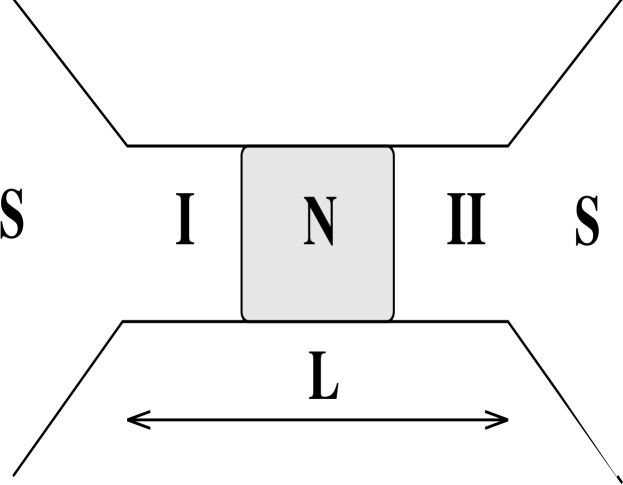
FIG. 1.: Schematic diagram of the mesoscopic disordered Josephson junction. I and II denote the portions of the contact region separated by the scattering region (hatched) where the motion of the quasiparticles is diffusive.

FIG. 2.: The quasiparticle current (a) and the differential conductance (b) versus voltage at various temperatures, for a disordered SNS junction. From top to bottom $T=0,1,2,3\Delta$. At low voltages, the dc current (a) has a square root dependence on voltage, while at high voltages exhibits excess current. The conductance (b) posseses subharmonic singularities, diverges at low voltages, and at high voltages asympotically tends to the normal state conductance of the disordered region.

FIG. 3.: The cosine (a) and sine (b) part of the first Fourier component of the ac current. From top to bottom (b) and from bottom to top (a) $T=0,1,2,3\Delta$. The slope at small voltages diverges as $(\Delta/V)^{1/2}$. See text for discussion about the high voltage behavior.

REFERENCES

- [1] A.W. Kleinsasser, R.E. Miller, W.H. Mallison and G.D. Arnold, Phys. Rev. Lett. 72, 1738 (1994).
- [2] N. van der Post, E.T. Peters, I.K. Yanson and J.M. van Ruitenbeek, Phys. Rev. Lett. 73, 2611 (1994).
- [3] A. Frydman and Z. Ovadyahu, Solid State Commun. 95, 79 (1995).
- [4] L.C. Mur, C.J.P.M. Harmans, J.E. Mooij, J.F. Carlin, A. Rudra, and M. Ilegems, Phys. Rev. B 54, R2327 (1996).
- [5] J. Kutchinsky, R. Taboryski, T. Clausen, C.B. Sorensen, A. Kristensen, P.E. Lindelof, J.B. Hansen, C.S. Jacobsen, and J.L. Skov, Phys. Rev. Lett. 78, 931 (1997).
- [6] E. Scheer, P. Joyez, D. Esteve, C. Urbina, and M.H. Devoret, Phys. Rev. Lett. 78, 3535 (1997).
- [7] E.N. Bratus’, V.S. Shumeiko, and G. Wendin, Phys. Rev. Lett. 74, 2110 (1995).
- [8] D. Averin and A. Bardas, Phys. Rev. Lett. 75, 1831 (1995).
- [9] U. Gunsenheimer and A.D Zaikin, Phys. Rev. B 50, 6317 (1994).
- [10] T.M. Klapwijk, G.E. Blonder, and M. Tinkham, Physica B 109-110, 1657 (1982).
- [11] A. Zaitzev, Sov. Phys. - JETP 51, 111 (1980).
- [12] A. Furusaki and M. Tsukada, Sol. State Commun. 78, 299 (1991).
- [13] C.W.J. Beenakker, Phys. Rev. Lett. 67, 3836 (1991).
- [14] S. Datta, P.F. Bagwell, M.P. Anatram, Phys. Low-Dim. Struct. 3, 1 (1996).
- [15] M.C. Koops, G.V. van Duyneveldt, and R. de Bruyn Ouboter, Phys. Rev. Lett. 77, 2542 (1996).
- [16] S.N. Artemenko, A.F. Volkov, and A.V. Zaitsev, Sov. Phys. - JETP 49, 924 (1979).
- [17] Yu. V. Nazarov, Phys. Rev. Lett. 73, 134 (1994).
- [18] A. Martín-Rodero, A. Levy Yeyati, and F.J. García-Vidal, Phys. Rev. B 53, R8891 (1996).
- [19] V.S. Shumeiko, E.N. Bratus’ and G. Wendin, Low Temp. Phys. 23, 181 (1997).
- [20] I.O. Kulik and A.N. Omel’yanchuk, JETP Lett. 21, 96 (1975).
- [21] K.M. Schep and G.E.W. Bauer, Phys. Rev. Lett. 78, 3015 (1997).
- [22] L.G. Aslamazov and A.I. Larkin Sov. Phys. - JETP 43, 698 (1976).
- [23] C. Nguyen, H. Kroemer, and E.L. Hu, Phys. Rev. Lett. 69, 2847 (1992).