Universality of the Gunn effect: self-sustained oscillations mediated by solitary waves

Abstract

The Gunn effect consists of time-periodic oscillations of the current flowing through an external purely resistive circuit mediated by solitary wave dynamics of the electric field on an attached appropriate semiconductor. By means of a new asymptotic analysis, it is argued that Gunn-like behavior occurs in specific classes of model equations. As an illustration, an example related to the constrained Cahn-Allen equation is analyzed.

In semiconductors where the local current density as a function of the local electric field is N-shaped, the Gunn effect is an ubiquitous phenomenon [1, 2, 3, 4, 5]. The Gunn effect [6] consists of time-periodic oscillations of the electric current flowing through an external purely resistive circuit attached to a semiconductor sample subject to dc voltage bias. The current oscillations correspond to the generation, one-dimensional motion and annihilation of solitary waves of the electric field inside the semiconductor. Besides this, the onset of the Gunn effect can be quite interesting, as the current may display intermittency accompanied by spatio-temporal structures of the electric field inside the semiconductor [7]. Recently the onset of the Gunn instability has been analyzed by singular perturbation methods which provide the governing amplitude equation for long semiconductors [8]. Gunn-like phenomena may also explain the experimentally-observed self-sustained oscillations of the current in doped weakly-coupled superlattices [9] whose dominant transport mechanism is resonant tunneling between adjacent quantum wells [10]. In these cases, the oscillations are due to recycling of electric field wavefronts (charge monopoles) instead of solitary waves [10]. The difference in the type of the waves may be tracked to the boundary condition at the injecting contact [11, 12]. Gunn-like phenomena have also been numerically observed in a driven diffusive lattice gas model of hopping conductivity [13].

A natural question that comes to mind in relation with these phenomena concerns their universality: Given that the Gunn instability appears in widely different semiconductor systems and models, what are the features a given model has to have in order to present the Gunn instability? Notice that the Gunn effect is in principle a nonequilibrium phenomenon which may happen far from any bifurcation points. Thus the question of its universality may not be related to linearization about fixed points of a renormalization transformation. Nevertheless a new asymptotic analysis allow us to understand deeply the Gunn effect and to try to give a precise meaning to the notion of universality far from equilibrium. This paper tries to give an answer to the universality question and it also puts the Gunn instability into perspective by comparing it to phenomena occurring in other pattern forming systems [14].

From the study of the Gunn instability in semiconductor models, we can extract the following common features that seem to be necessary for its occurrence:

1. The model should be able to support solitary waves moving in a privileged direction on a large enough spatial support.

2. It should include an integral (over space) constraint.

3. It should have appropriate boundary conditions (Dirichlet, Neumann, mixed, …) which render unstable the stationary solutions for certain values of the integral constraint.

We shall illustrate these points by constructing a simple model that displays the Gunn instability:

$$\frac{\partial u}{\partial t}+K\frac{\partial u}{\partial x}=\frac{\partial^{2}u}{\partial x^{2}}+J-g(u),$$ (1)

$${1\over L}\,\int_{0}^{L}u\,dx=\phi.$$ (2)

In these equations the unknowns are $u(x,t)$ and $J(t)$, with $t>0$ and $0<x<L$; $g(u)$ is a function having a local maximum $g_{M}=g(u_{M})$ followed by a local minimum $g_{m}=g(u_{m})$ for $u>0$ ($0<u_{M}<u_{m}$), while $K$ and $\phi$ are non-negative parameters. Equations (1)-(2) are to be solved with an appropriate initial condition for $u(x,0)\geq 0$ and Dirichlet boundary conditions:

$$u(0,t)=u(L,t)=\rho J(t),\ {g_{m}\over u_{m}}<{1\over\rho}<{g_{M}\over u_{M}}\,.$$ (3)

In semiconductor models $u$, $J$ and $\phi L$ correspond to the electric field, total current density and dc voltage bias, respectively. The boundary conditions (3) correspond to Ohm’s law relating the electric field and the current at the injecting and receiving contacts. (We assume that both contacts have identical resistivity $\rho>0$ for simplicity). Other boundary conditions (fixed $u$, mixed boundary conditions) do not qualitatively change the character of the solutions [1, 11].

FIG. 1.: (a) The function $J(t)$ for $g(u)=100(u-0.2)(u-0.4)(u-0.6)$. Parameter values are $K=2$, $L=100$, $\rho=1.5$ and $\phi=0.32$. (b) The corresponding profiles of $u(x,t)$ evaluated at the times marked in Part (a) of this figure. The minimum value of $J$ corresponds to $J^{*}=0$, whereas the plateau at intermediate values of $J$ corresponds to the solution of $2c_{+}(J)=c_{-}(J)$.

The model represented by Equations (1)-(2) with $K=0$ and zero-flux boundary conditions instead of (3) is known as the constrained Cahn-Allen equation, and it was recently introduced by Rubinstein and Sternberg as a nonlocal reaction-diffusion model of nucleation akin to the mass-conserving fourth-order Cahn-Hilliard equation [15, 16]. Equation (1) with a fixed constant $J$ and $K=0$ is the well-known bistable Fisher-Kolmogorov-Petrovskiǐ-Piskunov (FKPP) equation, which includes among its possible solutions a variety of traveling fronts and pulses (solitary waves) moving on an infinite 1 D spatial support [17, 14]. The pulses of the FKPP equation are unstable solutions: they either shrink or expand when an infinitesimal disturbance is added [17]. The global integral constraint (2) and Dirichlet boundary conditions (3) convert the FKPP equation in a model very similar to the typical semiconductor ones: the constrained Cahn-Allen equation. This model does not present the Gunn instability if $K=0$ because the $x\leftrightarrow-x$ symmetry implies no preferred direction of motion for traveling waves. A large enough nonzero convective term $K>0$ breaks the $x\leftrightarrow-x$ symmetry and it privileges waves moving from left to right. The resulting model satisfies the conditions 1 to 3 above and it displays the Gunn effect; see Fig. 1. It may be observed that the present model is also related to Kroemer’s model of the Gunn effect in n-GaAs [2]: we just change the convection coefficient to a constant $K$ in Ampère’s law and set the diffusivity equal to one in the dimensionless Kroemer’s model studied in Ref. [12]. These changes exclude the straightforward extension of our previous asymptotic analysis, as we cannot use the shock waves and particular solutions specific of Kroemer’s model to describe the Gunn effect [12].

To understand these results, we shall assume that $\epsilon=1/L\ll 1$. Then it is convenient to rewrite Equations (1)-(2) in terms of the ‘slow’ variables $s=\epsilon t$ and $y=\epsilon x$. The result is

$$\epsilon\frac{\partial u}{\partial s}+\epsilon K\frac{\partial u}{\partial y}-\epsilon^{2}\frac{\partial^{2}u}{\partial y^{2}}=J-g(u),$$ (4)

$$\int_{0}^{1}u\,dy=\phi.$$ (5)

In the limit $\epsilon\to 0$ the solutions of this system are piecewise constant: on most of the y-interval $u$ is equal to one or another of the zeros of $g(u)-J$, separated by transition layers that connect them. At $y=0$ and $y=1$ there are boundary layers (quasi-stationary most of the time), which we will call injecting and receiving layers, respectively. Let us assume that $u_{M}<\phi<u_{m}$ and denote by $u_{1}(J)<u_{2}(J)<u_{3}(J)$ the three zeros of $g(u)-J$. Let the initial profile $u(y,0)$ satisfying (5) be a square bump $u=u_{3}(J)$ for $Y_{1}(0)<y<Y_{2}(0)$ and $u=u_{1}(J)$ elsewhere plus terms of order $\epsilon$, as in the time marked by (1) in Fig. 1(b). Located at $y=Y_{1}$ and $y=Y_{2}$, $Y_{1}<Y_{2}$, there are sharp wavefronts of width $O(\epsilon)$ connecting $u=u_{1}(J)$ and $u=u_{3}(J)$. This initial profile will naturally evolve into the Gunn effect as time goes on (see below). The initial value of $J$ follows from (5):

$$\phi=u_{1}(J)+[u_{3}(J)-u_{1}(J)]\,(Y_{2}-Y_{1})+O(\epsilon).$$ (6)

The boundary layers and the fronts connecting $u_{1}(J)$ and $u_{3}(J)$ are built from trajectories of the phase plane:

$$\frac{du}{d\xi}=v;\ \frac{dv}{d\xi}=\mu v+g(u)-J,$$ (7)

where $\xi=\epsilon^{-1}[y-Y_{i}(s)]$, $c=dY_{i}/ds$ and $\mu=K-c$. The boundary layers are separatrices connecting the vertical line $u=\rho J$ in the phase plane $(u,v)$ to the saddles $(u_{1},0)$ or $(u_{3},0)$ for $c=0$: $u(x)\to u_{i}(J)$ as $x\to\infty$ and $u(x)\to u_{i}(J)$ as $(x-L)\to-\infty$ ($i=1,3$) are the matching conditions. For each fixed value of $J$ between $g_{m}$ and $g_{M}$ we can find a unique value $c_{+}(J)$ such that $u(-\infty)=u_{1}(J)$ and $u(\infty)=u_{3}(J)$ [corresponding to a heteroclinic orbit connecting $(u_{1},0)$ to $(u_{3},0)$ with $v>0$] and a unique value $c_{-}(J)$ such that $u(-\infty)=u_{3}(J)$ and $u(\infty)=u_{1}(J)$ [a heteroclinic orbit connecting $(u_{3},0)$ to $(u_{1},0)$ with $v<0$]. The functions $c_{\pm}(J)$ are depicted in Fig. 2. They intersect when $J=J^{*}$ given by

$$J^{*}=\frac{1}{u_{3}-u_{1}}\,\int_{u_{1}}^{u_{3}}g(u)\ du,\quad c_{\pm}=K.$$ (8)

FIG. 2.: The functions $c_{\pm}(J)$ for $K=2$, and $g(u)$ as in Fig. 1. When $J_{c}>J^{{\dagger}}$ (vertical line at $J=J^{{\dagger}}$) only one wave is shed during each period, whereas multiple shedding may occur for $J^{*}<J_{c}<J^{{\dagger}}$.

Starting at $s=0$, the fronts $Y_{i}(s)$ move with speeds

$${dY_{1}\over ds}=c_{+}(J),\quad{dY_{2}\over ds}=c_{-}(J),$$ (9)

whereas their positions are related to the bias $\phi$ through (6). We find an equation for $J$ by differentiating (6) and then inserting (9) in the result:

$${dJ\over ds}=A(J)\,[c_{+}(J)-c_{-}(J)],$$ (10)

$$A=\frac{(u_{3}-u_{1})^{2}}{{\phi-u_{1}\over g^{\prime}_{3}}+{u_{3}-\phi\over g^{\prime}_{1}}}\,>0,$$ (11)

where $g^{\prime}_{i}\equiv g^{\prime}(u_{i})$ and we have used that $g(u_{i}(J))=J$ implies $\partial u_{i}/\partial J=1/g^{\prime}(u_{i})$. This is a simple equation for $J$ demonstrating that $J$ tends to $J^{*}$ exponentially fast. Notice that this is a very simple explanation of the well-known observation that a pulse detached from the boundaries moves at constant speed and $J$, given by the equal area rule (8).[1]

After a certain time, the wavefront $Y_{2}$ reaches 1 and we have a new stage governed by (6) with $Y_{2}=1$ and $Y_{1}$ given by (9). The equation for $J$ becomes $dJ/ds=A\,c_{+}>0$ and its solution increases [compare $J$ and $u$ at time (2) in Fig.  1] until it surpasses the value $J_{c}$ such that $u_{2}(J)=\rho J$. (At $J_{c}$, $[\partial u/\partial x]_{x=0}$ changes sign and the quasistationary injecting layer becomes unstable)[12]. Let $s_{1}$ be the earliest time at which $J=J_{c}$. After $s=s_{1}$, the profile of $u$ changes within the boundary layer at $y=0$: this injecting layer becomes unstable and it sheds a new wave during a fast stage described by the time scale $\tau=(s-s_{1})/\epsilon$. To find what happens next we need to perform a more complicated analysis keeping $O(\epsilon)$ terms in the outer (bulk) expansion of $u$ and $J$ and just the leading-order term in all inner expansions (boundary layers and wavefronts). This calculation has been performed in detail for a semiconductor model. [18] It can be shown that the shedding of a new wave from the injecting layer is governed by the following semi-infinite problem for $x>0$, $-\infty<\tau<\infty$: $u(x,\tau)$ (far from the old wave dying at $y=1$) solves (1) and $u(0,\tau)=\rho J(\tau;\epsilon)$, with $J(\tau;\epsilon)=J_{c}+\epsilon J^{(1)}(\tau)$,

$$J^{(1)}(\tau)=h^{\prime}(\tau)+\alpha h(\tau)-\gamma\int_{-\infty}^{\tau}e^{-\beta(\tau-t)}\,h(t)\,dt,$$ (12)

$$h(\tau)=(u_{3}-u_{1})\,c_{+}\,(\tau-\tau_{0})-\int_{0}^{\infty}[u(x,\tau)-u_{1}]\,dx,$$ (13)

(in this equation all functions of $J$ are calculated at $J=J_{c}$; $\tau_{0}$ is a constant and $\alpha$, $\beta$ and $\gamma$ are positive parameters)[18] and the following matching condition on an appropriate overlap domain: $u(x,\tau)-u_{0}(x;J(s))\ll 1$, as $\tau\to-\infty,\,s\to s_{1}-$. Here $u_{0}(x;J(s))$ is the quasistationary injecting layer solution of (7) with $\mu=K$ such that $u_{0}(0;J(s))=\rho J(s)$ and $u_{0}(\infty;J(s))=u_{1}(J(s))$ for $s<s_{1}$, $J(s_{1})=J_{c}$. The function $h(\tau)$ is the area lost due to the motion of the old front during the time $\tau$ minus the instantaneous excess area under the injecting layer.

The solution of the previous semi-infinite problem reveals the formation, growth and motion of a new pulse in the injecting layer, driven by $h(\tau)$ through the effective excess current (12). This process ends when the new pulse is bounded by two well-formed wavefronts (detached from the injecting layer) which are located at $Y_{3}$ and $Y_{4}$, $Y_{3}<Y_{4}$ [see the $u$-profile at time (3) in Fig.  1(b) in which $Y_{3}$ and $Y_{4}$ have already moved from their initial positions $O(\epsilon\ln\epsilon)$ at the beginning of this stage]. It may be seen that the injecting layer becomes unstable and sheds a new wave when its width reaches a critical size $\Delta y=O(\epsilon\ln\epsilon)$ [18].

If $\phi$ is large enough, we have a stage where the old wavefront located at $Y_{1}<1$ coexists with the newly formed pulse bounded by the two wavefronts located at $Y_{3}$ and $Y_{4}$:

$$\phi=u_{1}(J)+[u_{3}(J)-u_{1}(J)]\,(1-Y_{1}+Y_{4}-Y_{3})$$ (14)

$$+O(\epsilon).$$ (15)

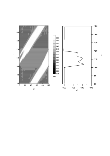
FIG. 3.: (a) Density plot for u(x,t) with $\rho=4$, $\phi=0.3$ and $g(u)$ as in Fig. 1 (lighter color means larger $u$). Here multiple shedding of pulses occurs at the injecting layer: two pulses are formed during each period. The secondly shed reaches and overtakes the first one. (b) The corresponding profile of $J(t)$.

Differentiating this equation and using that $Y_{1}$ and $Y_{3}$ move with speed $c_{+}$ whereas $Y_{4}$ moves with speed $c_{-}$, we obtain $dJ/ds=A\,(2c_{+}-c_{-})$. Starting from $J_{c}$, $J$ decreases further to $J^{{\dagger}}$ [the zero of $(2c_{+}-c_{-})$] if $2c_{+}(J_{c})<c_{-}(J_{c})$ (the stable case with $J_{c}>J^{{\dagger}}$ in Fig. 2). After the old wave reaches $y=1$, we get again Equations (6)-(10) and recover the initial situation. Thus a full period of the Gunn oscillation is described; see Fig. 1. On the other hand, if $2c_{+}(J_{c})>c_{-}(J_{c})$ ($J^{*}<J_{c}<J^{{\dagger}}$), $J$ increases after the formation of the new pulse and it is possible for the injecting layer to shed more waves into the bulk as shown by the numerical simulations of Fig. 3. How many waves are shed depends both on the value of $J_{c}$ (and therefore on the injecting resistivity $\rho$) and on the length $L$. A rough estimation would give $(n+1)\,c_{+}(J_{c})=n\,c_{-}(J_{c})$ as $\epsilon\to 0$ for the number $n$ of shed waves. This shedding mechanism seems to have the effect of breaking the spatial coherence of the sample which may lead to complex spatio-temporal phenomena (intermittencies with a varying number of pulses present in the sample at different times). The unstable case will be further analyzed in the near future.

In conclusion we have investigated what are the main features that a given model should have in order to present the Gunn effect. These features are demonstrated by studying a simple model by means of a general asymptotic analysis corroborated by direct numerical simulations. As a result the Gunn effect is reduced to solving a sequence of very simple problems (one equation for $J$ each time) plus a canonical problem for shedding new pulses. Our asymptotic analysis explains qualitative and quantitativally the formation, motion and annihilation of pulses in the Gunn effect. This work sheds light on several puzzling aspects of the Gunn oscillations (see the Chapter on open problems in Ref. [22]): (i) why do pulses move with the well-known equal-area-rule velocity at constant $J$ when they are far from the contacts? [the corresponding current is a stable equilibrium of (10)]; (ii) how does the wavespeed change when it arrives to the receiving contact?; (iii) how are new waves created at the injecting contact? In addition we have described a new instability mechanism consisting of multiple pulse shedding during each oscillation of $J$, which appears for appropriate values of the boundary parameters at the injecting contact. Similar work has been performed in diverse semiconductor models: Gunn oscillations in ultrapure closely compensated p-Ge [18], Kroemer’s model of Gunn oscillations in bulk n-GaAs [19] and slow oscillations in semi-insulating GaAs [20]. A modification of the asymptotic method presented here describes the charge monopole recycling responsible for the self-oscillations in n-doped weakly coupled superlattices [21]. Irrespective of the physical mechanism responsible for the existence of wavefront and pulses, our asymptotic method describes the Gunn oscillations in these models. The model presented here perhaps illustrates in the simplest way what the method consists of: (i) find the equations and boundary conditions which characterize the shape of the wavefronts and their speed as functions of the current density $J$; (ii) derive the equations which determine $J$ as a function of the slow time scale depending on the number of wavefronts present in the sample. The field profile follows adiabatically the evolution of $J$; and (iii) add the semiinfinite problems responsible for wave shedding at the contacts. Solution and matching of these problems yields an approximation to the Gunn effect in the given model. Of course solving some of these steps may be in itself a rather complicated technical problem for particular models requiring special asymptotics [20].

- [1] M. P. Shaw, V. V. Mitin, E. Schöll and H. L. Grubin, The Physics of Instabilities in Solid State Electron Devices, (Plenum Press, 1992, New York).
- [2] H. Kroemer, in Topics in Solid State and Quantum Electronics, edited by W. D. Hershberger (John Wiley, N. Y. 1972), p. 20.
- [3] M. J. Bergmann, S. W. Teitsworth, L. L. Bonilla and I. R. Cantalapiedra, Phys. Rev. B 53, 1327 (1996).
- [4] H. Le Person, C. Minot, L. Boni, J. F. Palmier, and F. Mollot, Appl. Phys. Lett. 60, 2397 (1992).
- [5] V. A. Samuilov, in Nonlinear Dynamics and Pattern Formation in Semiconductors and Devices, edited by F.-J. Niedernostheide (Springer Verlag, Berlin, 1995), p. 220.
- [6] J. B. Gunn, Solid State Commun. 1, 88 (1963).
- [7] A. M. Kahn, D. J. Mar and R. M. Westervelt, Phys. Rev. B 43, 9740 (1991) and Phys. Rev. B 45, 8342 (1992).
- [8] L. L. Bonilla and F. J. Higuera, SIAM J. Appl. Math., 55, 1625 (1995).
- [9] J. Kastrup, H.T. Grahn, R. Hey, K. Ploog, L. L. Bonilla, M. Kindelan, M. Moscoso, A. Wacker and J. Galán, Phys. Rev. B 55, 2476 (1997).
- [10] L. L. Bonilla, in Nonlinear Dynamics and Pattern Formation in Semiconductors and Devices, edited by F.-J. Niedernostheide (Springer Verlag, Berlin, 1995), p. 1.
- [11] H. Kroemer, IEEE Trans. ED-15, 819 (1968).
- [12] F. J. Higuera and L. L. Bonilla, Physica D 57, 161 (1992).
- [13] C. Maes and W. Vanderpoorten, Phys. Rev. B 53, 12889 (1996).
- [14] M. C. Cross and P. C. Hohenberg, Rev. mod. Phys. 65, 851 (1993).
- [15] J. Rubinstein and P. Sternberg, IMA J. Appl. Math. 48, 249 (1992).
- [16] While the Cahn-Hilliard equation is the simplest gradient flow which conserves mass and is local, the constrained Cahn-Allen equation is a simple nonlocal gradient flow that conserves mass. See a discussion and comparison of the two models in Ref. 15. A nice analysis of the front motion in the 1 D Cahn-Allen model can be found in the paper: L. G. Reyna and M. J. Ward, European J. Appl. Math. 5, 495 (1994).
- [17] J. D. Murray, Mathematical Biology, Biomathematics 19, (Springer Verlag, 1990, New York), Chapter 11. P. C. Fife, Mathematical Aspects of Reacting and Diffusing Systems, Lecture Notes in Biomathematics 28, (Springer Verlag, 1979, New York).
- [18] L. L. Bonilla, P. J. Hernando, M. A. Herrero, M. Kindelan and J. J. L. Velázquez, Physica D (1997), to appear.
- [19] L. L. Bonilla, I. R. Cantalapiedra, G. Gomila and J. M. Rubí, Phys. Rev. E (1997), to appear, manuscript EC6362. See also, G. Gomila, J. M. Rubí, I. R. Cantalapiedra and L. L. Bonilla, Phys. Rev. E (1997), to appear, manuscript EC6361.
- [20] L. L. Bonilla, P. J. Hernando and M. Kindelan, unpublished.
- [21] L. L. Bonilla, M. Kindelan, M. Moscoso and S. Venakides, SIAM J. Appl. Math. 57(6) (1997), to appear.
- [22] V. L. Bonch-Bruevich, I. P. Zvyagin and A. G. Mironov, Domain electrical instabilities in semiconductors, (Consultants Bureau, 1975, New York).