Neural Networks

Abstract

We review the theory of neural networks, as it has emerged in the last ten years or so within the physics community, emphasizing questions of biological relevance over those of importance in mathematical statistics and machine learning theory.

1 Introduction

Understanding at least some of the functioning of our own brain is certainly an extraordinary scientific and intellectual challenge and it requires the combined effort of many different disciplines. Each individual group can grasp only a limited set of aspects, but its particular methods, questions and results can influence, stimulate and hopefully enrich the thoughts of others. This is the frame in which the following contribution, written by theoretical physicists, should be seen.

Statistical physics usually deals with large collections of similar or identical building blocks, making up a gas, a liquid or a solid. For the collective behavior of such an assembly most of the properties of the individual elements are only of marginal relevance. This allows to construct crude and simplified models which nevertheless reproduce certain aspects with extremely high accuracy. An essential part of this modeling is to find out which of the properties of the elements are relevant and what kind of questions can or cannot be treated by such models. The usual goal is to construct models as simple as possible and to leave out as many details as possible, even if they are perfectly well known. The natural hope is that the essential properties can be understood better on a simple model. This, on the other hand, seems to contrast the ideals of modeling in other disciplines and this can severely obstruct the interdisciplinary exchange of thoughts.

Our brain ([Brai]) is certainly not an unstructured collection of identical neurons. It consists of various areas performing special tasks and communicating along specific pathways. Even on a smaller scale it is organized into layers and columns. Nevertheless the overwhelming majority of neurons in our brain belongs to one of perhaps three types. Furthermore, on an even smaller scale, neurons seem to interact in a rather disordered fashion, and the pathways between different areas are to some degree diffuse. Keeping in mind that models of neural networks with no a priori structure are certainly limited, it is of interest to see how structures can evolve by learning processes and what kind of tasks they can perform.

Over the last ten or more years, abstract and simplified models of brain functions have been a target of research in statistical physics ([Amit]; [HKP]). A model of an associative memory was proposed by Hopfield in 1982, following earlier work by Caianello and Little. This model is not only based on extremely simplified neurons (McCulloch-Pitts, 1943), it also serves a heavily schematized task, the storage and retrieval of uncorrelated random patterns. This twofold idealization made it, however, tractable and accessible for quantitative results. In the meantime there have been many extensions of this model, some of which will be discussed later on. One of the essential points of this model is the fact that information is stored in a distributed fashion in the synaptic connections among the neurons. Each synapse carries information about each pattern stored, such that destruction of part of the synapses does not destroy the whole memory. The storage of a pattern requires a learning process which results in a modification of the strength of all synapses. The original model was based on a simple learning rule, essentially the one proposed by Hebb, which is in a sense a neuronal manifestation of Pawlow’s ideas of conditional reflexes. Regarding learning, again more sophisticated rules have been investigated and are discussed later.

Even restricting ourselves to this kind of models, we can sketch only a small part of what has been worked out in the past, and only small parts also of the progress in getting those models closer to biology. It is interesting to note that artificial neural nets, in the form of algorithms or hardware, have found many technical applications. This aspect will, however, be left aside almost completely.

Before entering the discussion of learning or memory, we want to give a brief overview over the biological background of neurons, their basic functioning and their arrangement in the brain ([Brai]; [Abe]).

2 Biological vs. Formal Neural Nets

2.1 Biological Background

A typical neuron, e.g. a pyramidal cell (see Fig. 1 next page), consists of the cell body or soma; extending from it there is a branched structure of about 2 mm diameter, called dendrite, and the nerve fiber or axon, which again branches and can have extensions reaching distant parts of the brain. The branches of the axon end at so called synapses which make contact to the dendrites of other neurons. There are of course also axons coming in from sensory organs or axons reaching out to the motor system. Compared to the number of connections within the brain, their number is rather small. This amazing fact indicates perhaps that the brain is primarily busy analyzing the sparse input or shuffling around internal information.

The main purpose of a neuron is to receive signals from other neurons, to process the signals and finally to send signals again to other cells. What happens in more detail is the following. Assume a cell is excited, which means that the electrical potential across its membrane exceeds some threshold. This creates a short electric pulse, of about 1 msec duration, which travels along the axon and ultimately reaches the synapses at the ends of its branches. Having sent a spike, the cell returns to its resting state. A spike arriving at a synapse releases a certain amount of so called neuro–transmitter molecules which diffuse across the small gap between synapse and dendrite of some other cell. The neuro–transmitters themselves then open certain channel proteins in the membrane of the postsynaptic cell and this finally influences the electrical potential across the membrane of this cell. The neuro–transmitters released from pyramidal cells have the effect of driving the potential of the postsynaptic cell towards the threshold, their synapses are called excitatory. There are, however, also inhibitory cells with neuro–transmitters having the opposite effect. The individual changes of the potential caused by the spikes of the presynaptic cells are collected over a period of about 10 msec and if the threshold is reached the postsynaptic cell itself fires a spike. Typically 100 incoming spikes within this period are necessary to reach this state.

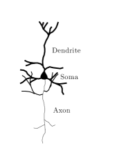
Figure 1: Schematic view of a neuron

The human brain contains $10^{10}$ to $10^{11}$ neurons and more than $10^{14}$ synaptic connections among them. The neurons are arranged in a thin layer of about 2 mm on the surface, the cortex, and each mm² contains typically $10^{5}$ such cells. This means that the dendritic trees of these cells penetrate each other and form a dense web. Part of the axons of these cells again project onto the dendrites in the immediate neighborhood and only a fraction reaches more distant regions of the brain. This means that on a scale of a few mm³ more than $10^{5}$ neurons are tightly connected. This does not imply that more distant regions are weakly coupled. The huge amount of white matter containing axons connecting more distant parts only indicates the possibility of strong interactions of such regions as well.

It is tempting to compare this with structures which we find within the integrated circuits of an electronic computer. The typical size of a synapse is 0.1 $\mu$m, whereas the smallest structures found in integrated circuits are about five times as big. The packing density of synapses attached to a dendrite is about $10^{9}$ per mm², whereas only $1/1000$ of this packing density is reached in electronic devices. A comparison of the computational power is also impressive. A modern computer can perform up to $10^{9}$ elementary operations per sec. The computational power of a single neuron is rather low, but they all work in parallel. Assuming that a neuron fires with a rate of 10 spikes per sec, which is typical, and assuming that each spike transmitted through a synapse corresponds to an elementary computation, we find a computing power of about $10^{15}$ operations per second. These numbers have to be kept in mind if we try to imitate brain functions with artificial devices.

2.2 Formal Neurons — Spikes vs. Rates

The actual processes going on when a spike is formed or when it arrives at a synapse and its signal is transmitted to the next neuron, involve an interplay of various channels, ionic currents and transmitter molecules. This should not be of concern as long as we are interested only in the data processing aspects. A serious question is, however, what carries the information? Is it a single spike and its precise timing or is the information coded in the firing rates? For sensory neurons the proposition of rate coding seems well established. These neurons typically have rather high firing rates in their excited state. For the brain this is much less clear since the typical spike rates are low and the intervals between two successive spikes emitted by a neuron are longer or at best of the order of the time over which incoming spikes are accumulated. Nevertheless a spike rate coding is usually assumed for the brain as well. This means that a rate has to be considered as an average over the spikes of many presynaptic neurons rather than a temporal average over the spikes emitted by a single cell. This is plausible, having in mind that typically 100 or more arriving spikes are necessary to release an outgoing spike. This suggests for the firing rate $\nu_{i}$ of a neuron $i$

$$\nu_{i}(t)=\Phi\left(\sum_{j}W_{ij}\nu_{j}(t)-\vartheta\right)\ ,$$ (1)

where $\vartheta$ is some threshold and $\Phi(x)$ is some increasing function of $x$. The simplest assumption is $\Phi(x)=0$ for $x<0$ and $\Phi(x)=1$ for $x>0$. This model was first proposed by McCulloch and Pitts (1943). The quantity $W_{ij}$ describes the coupling efficacy of the synapse connecting the presynaptic cell $j$ with the postsynaptic cell $i$. For excitatory synapses $W_{ij}>0$, and for inhibitory synapses $W_{ij}<0$.

This model certainly leaves out many effects. For instance the assumption of linear superposition of incoming signals neglects any dependence on the position of the synapse on the dendritic tree.

Investigating networks of spiking neurons, one has again designed simplified models. One of them is the integrate and fire neuron which mimics the mechanism of spike generation at least in a crude way. It sums up incoming signals by changing the membrane potential. As soon as a certain threshold is reached, the neuron fires and the membrane potential is reset to its resting value.

If rate coding is appropriate, results obtained for the first kind of networks should be reproduced by networks of spiking neurons as well. On the other hand there are many questions which can only be taken up within the framework of spiking neurons, for instance which role the precise timing of spikes plays ([Abe]) or whether the activity in a network with excitatory couplings among its neurons can be stabilized by adding inhibitory neurons ([AB]).

2.3 Hebbian Learning — Sparse Coding

The most remarkable feature of neural networks is their ability to learn. This is attributed to a certain plasticity of the synaptic coupling strengths. The question is of course, how is this plasticity used in a meaningful way?

The basic idea proposed by Hebb (1949) actually goes back to the notion of conditional reflexes put forward by Pawlow. Assume a stimulus $A$ results in a reaction $R$. If simultaneously with $A$ a second stimulus $B$ is applied, then after some training stimulus $B$ alone will be sufficient to trigger reaction $R$, although this was not the case before training. Let $A$ be represented by the activity of a neuron $\ell$ and the reaction $R$ by neuron $i$ becoming active. This would be the case if the coupling $W_{i\ell}$ is sufficiently strong. Before training, the stimulus $B$, represented by the activity of neuron $j$, is assumed not to trigger the reaction $R$. That is, the coupling $W_{ij}$ is assumed to be weak. During training with $A$ and $B$ present, the cells $j$ and $i$ are simultaneously active, the latter being activated by cell $\ell$. Assume now that the synaptic strength $W_{ij}$ between neurons $j$ and $i$ is increased, if both cells are simultaneously active. Then, after some training, this coupling $W_{ij}$ will be strong enough to sustain the reaction $R$ without $A$ being applied, provided $B$ is present. This is represented by the Hebb learning rule

$$\Delta W_{ij}\propto\nu_{i}\,\nu_{j}$$ (2)

Most remarkably this learning rule does not require a direct connection between the cells $\ell$ and $j$ representing the stimuli $A$ and $B$. That is, the equivalence of stimuli $A$ and $B$ has been learnt without any a priori relation between $A$ and $B$. What has been used is only the simultaneous occurrence of $A$ and $B$. Despite its simplicity this learning rule is extremely powerful.

It is not completely clear how such a change in the synaptic efficacies is realized in detail, whether it is caused by changes in the synapse itself or by changes in the density of receptor proteins on the membrane of the dendrite of the postsynaptic neuron. Nevertheless it is plausible at least in the sense that this learning process depends only on the simultaneous state of the pre- and postsynaptic cell. It is generally assumed that learning takes place on a time scale much slower than the intrinsic time scale of a few msec characteristic of neural dynamics.

We can now go one step further and consider the learning of more than one pattern. A pattern is a certain configuration of active and inactive neurons. A pattern, say $\mu$, is represented by a set of variables $\xi_{i}^{\mu}$ for each pattern and neuron. This means that in pattern $\mu$ neuron $i$ fires with a rate $\xi_{i}^{\mu}$. In the most simple case $\xi_{i}^{\mu}=1$ if $i$ is excited and $\xi_{i}^{\mu}=0$ otherwise. Having learnt a set of patterns the couplings, according to the above learning rule, have the values

$$W_{ij}=W_{o}\sum_{\mu}\xi_{i}^{\mu}\,\xi_{j}^{\mu}$$ (3)

where $W_{o}$ has the meaning of a learning strength. Actually this learning strength might also depend on the kind of pattern presented, for instance on whether the pattern is new, unexpected, relevant in some sense or under which global situation, attention, laziness or stress, it is presented. This can lead to improved learning or suppression of uninteresting information.

The above learning rule is constructed such that, at least for $W_{o}>0$, only excitatory couplings are generated. This is in accordance with the finding that the pyramidal neurons have excitatory synapses only and that the plasticity of the synapses is most pronounced in this cell type. This causes, on the other hand, a problem. A network with excitatory synapses only would shortly go into a state where all neurons are firing at a high rate. The cortex contains, however, inhibitory cells as well. The likely purpose of these cells is to control the mean activity of the network and to prevent it from reaching the unwanted state of uniform high activity. A malfunctioning of this regulation is probably the cause of epileptic seizures.

Actually the mean activity in our brain seems to be rather low. This means that at a given time only a small percentage of the neurons is firing at an elevated rate. Typical patterns are sparse, having many more $0$’s than $1$’s. This is a bit surprising since the maximal information per pattern is contained in binary patterns with approximately equal number of $0$’s and $1$’s and such symmetric coding is also used in our computers. Nevertheless there are several good reasons for sparse coding, some of which will be discussed later.

In the original Hopfield model the degree of abstraction is pushed a step further. Here symmetric patterns with equal number of $0$’s and $1$’s are considered. This requires a modified learning rule. First of all the inactive state is now represented by $-1$ rather than $0$. With this modification the above learning rule can again be used, but now the coupling strength can also be weakened and the couplings can acquire negative values. Furthermore it is assumed that each neuron is connected to every other neuron and that the couplings between two neurons have the same value in both directions. This is certainly rather unrealistic in view of the biological background. Modified models with one or the other simplifying assumption removed have been investigated as well. They show, however, quite similar behavior. This demonstrates the robustness of the models with respect to modifications of details, which might again serve as a justification of this simple kind of modeling.

2.4 Transmission Delays

The propagation of a spike along the axon, the transmission of this signal across the synapse and the propagation along the dendrite take some time. This causes some total delay $\tau_{ij}$, typically a few msec, in the transmission of a signal from neuron $j$ to neuron $i$. Incorporating this into eq.(1) yields a modified form

$$\nu_{i}(t)=\Phi\left(\sum_{j}W_{ij}\nu_{j}(t-\tau_{ij})-\vartheta\right).$$ (4)

As long as we are interested in slow processes, this delay is of no relevance. On the other hand it gives the opportunity to generate or learn sequences of patterns evolving in time. This might be of relevance in processes like speech generation or recognition, or in generating periodic or aperiodic motions. Other proposals use this mechanism for temporal linking of different features of the same object or for the segmentation of stimuli generated by unrelated objects. Another mechanism which might play a role in this context is the phenomenon of fatigue. This means that the firing rate of an excited neuron, even at constant input, goes down after a while. The associated time scales can vary from few msec up to minutes or hours. In any case there are several mechanisms which can be used for the generation or recognition of temporal structures and we are coming back to this point later.

The picture developed so far certainly leaves out many interesting and important aspects. Nevertheless even this oversimplified frame allows to understand some basic mechanisms. On the other hand it is far from a description of the brain as a whole. What is certainly missing, is the structure on a larger scale. In order to proceed in this direction one would have to construct modules performing special tasks, like data preprocessing or memory, and one would have to arrange for a meaningful interplay of those modules. This is currently far beyond our possibilities, as we are lacking analytic tools or computational power and, perhaps more importantly even, good questions and well formalizable tasks to be put to such a modular architecture.

3 Learning and Generalization

Given that we interpret the firing patterns of a neural network as representing information, neural dynamics must be regarded as a form of information processing. Moreover, disregarding the full complexity of the internal dynamics of single neurons, as we have good reasons to do (see Sec. 2.2), we find the course of neural dynamics, hence information processing in a neural networks, being determined by its synaptic organization.

Consequently, shaping the information processing capabilities of a neural network requires changing its synapses. In a neural setting, this process is called “learning”, or “training”, as opposed to “programming” in the context of symbolic computation. Indeed, as we have already indicated above, the process of learning is rather different from that of programming a computer. It is incremental, sometimes repetitive, and it proceeds by way of presenting “examples”. The examples may represent associations to be implemented in the net. They may also be instances of some rule, and one of the reasons for excitement about neural networks is that they are able to extract rules from examples. That is, by a process of training on examples they can be made to behave according to a set of rules which — while manifest in the examples — are usually never made explicit, and are quite often not known in algorithmic detail. Such is, incidentally, also the case with most skills humans possess (subconcsiously). In what follows, we discuss the issues of learning and generalization in somewhat greater detail.

We start by analysing learning (and generalization) for a single threshold neuron, the perceptron. First, because it gives us the opportunity to discuss some of the concepts useful for a quantitative analysis of learning already in the simplest possible setting; second, because the simple perceptron can be regarded as the elementary building block of networks exhibiting more complicated architectures, and capable of solving more complicated tasks.

Figure 2: (a) Feed–forward Network. (b) Network with feed–back loops

Regarding architectures, it is useful to distinguish between so called feed–forward nets, and networks with feedback–loops (Fig. 2). In feed–forward nets, the information flow is directed; at their output side, they produce a certain map or function of the firing patterns fed into their input layer. Given the architecture of such a layered net, the function it implements is determined by the values of the synaptic weights between its neurons. Networks with feedback–loops, on the other hand exhibit and utilize non–trivial dynamical properties. For them, the notion of (dynamical) attractor is of particular relevance, and learning aims at constructing desired attractors, be they fixed points, limit cycles or chaotic. We discuss attractor networks separately later on in Sec. 4. Finally, feed–forward architectures may be combined with elements providing feedback–loops in special ways to create so–called feature maps, which we also briefly describe.

The physics–approach to analyzing learning and generalization has consisted in supplementing general considerations with quantitative analyses of heavily schematized situations. Main tools have been statistical analyses, which can however be quite forceful (and luckily often simple) when the size of a given information processing task becomes large in a sense to be specified below.

It goes without saying that this approach would not be complete without demonstrating — either theoretically, by way of simulations, or, by studying special examples — that the main functional features and trends seen in abstract statistical settings would survive the removal of a broad range of idealizations and simplifications, and that they, indeed, prove to be resilient against changing fine details at the microscopic level.

3.1 Simple Perceptrons

A perceptron mimics the functioning of a single (formal) neuron. Given an input $\vec{\nu}=(\nu_{1},\nu_{2},\dots,\nu_{N})$ at its $N$ afferent synapses, it evaluates its local field or post-synaptic potential as weighted sum of the input components $\nu_{j}$,

$$h_{0}(\vec{\nu})=\sum_{j=1}^{N}W_{0j}\nu_{j}\ ,$$ (5)

compares this with a threshold $\vartheta$, and produces an output $\nu_{0}$ according to its transfer function or input–output relation

$$\nu_{0}=\Phi(h_{0}(\vec{\nu})-\vartheta)\ ,$$ (6)

For simple perceptrons, one usually assumes a step–like transfer function. Common choices are $\Phi(x)={\rm sgn}(x)$ or $\Phi(x)=\Theta(x)$ depending on whether one chooses a $\pm 1$ representation or a 1–0 representation for the active and inactive states.

Figure 3: Linear separation by a perceptron

The kind of functionality provided by a perceptron has a simple geometrical interpretation. Equation (6) shows that a perceptron implements a two-class classification, assigning an ‘active’ or an ‘inactive’ output–bit to each input pattern $\vec{\nu}$, according to whether it produces a super- or sub–threshold local field. The dividing decision surface is given by the inputs for which $\vec{W}_{0}\cdot\vec{\nu}\equiv\sum_{j}W_{0j}\nu_{j}=\vartheta$. It is a linear hyperplane orthogonal to the direction of the vector $\vec{W}_{0}$ of synaptic weights $(W_{0j})$ in the $N$-dimensional space of inputs (Fig. 3). Pattern sets which are classifiable that way are called linearly separable. The linearly separable family of problems is certainly non–trivial, but obviously also of limited complexity. Taking Boolean functions of two inputs as an example, and choosing the representation $1\equiv{\em true}$ and $0\equiv{\em false}$, one finds that ${\rm AND}(\nu_{1},\nu_{2})$, and ${\rm OR}(\nu_{1},\nu_{2})$ as well as ${\rm IMPL}(\nu_{1},\nu_{2})$ are linearly separable, whereas ${\rm XOR}(\nu_{1},\nu_{2})$ is not.

It is interesting to see, how Hebbian learning, the most prominent candidate for a biologically plausible learning algorithm, would perform on learning a linearly separable set of associations. A problem that has been thoroughly studied is that of learning random associations. That is, one is given a set of input patterns $\vec{\xi}^{\mu}$, $\mu=1,\dots,P$, and their associated set of desired output labels $\zeta_{0}^{\mu}$. Each bit in each pattern is independently chosen to be either active or inactive with equal probability and the same is assumed for the output bits.

It has been known for some time ([cov]) that such a set of random associations is typically linearly separable, as long as the number $P$ of patterns does not exceed twice the dimension $N$ of the input space, $P\leq 2N$. It turns out that the suitable representation of the active and inactive states for this problem — i.e., appropriate for the given pattern statistics — is a $\pm 1$ representation. Moreover, due to the symmetry between active and inactive states in the problem, a zero threshold should be chosen.

Learning à la Hebb by correlating pre- and postsynaptic activities, one has $(\Delta W_{0j})^{\mu}\propto\zeta_{0}^{\mu}\xi_{j}^{\mu}$ as the synaptic change in response to a presentation of pattern $\mu$. As we have mentioned already, this involves a modification of Hebb’s original proposal. Summing contributions from all patterns of the problem set, one obtains (compare Eq. (3))

$$W_{0j}=\frac{1}{N}\sum_{\mu=1}^{P}\zeta_{0}^{\mu}\xi_{j}^{\mu}\ ,$$ (7)

where the prefactor is chosen just to fix scales in a manner that allows taking a sensible large system limit. Here we distinguish input from output bits by using different symbols for them. In recursive networks, outputs of single neurons are used as inputs by other neurons of the same net, and the distinction will be dropped in such a context.

It is not difficult to demonstrate that Hebbian learning finds an approximation to the separating hyperplane, which is rather good for small problem size $P$, but which becomes progressively worse as the number of patterns to be classified increases. To wit, taking an arbitrary example $\vec{\xi}^{\nu}$ out of the set of learnt patterns, one finds that the Hebbian synapses (7) produce a local field of the form $h^{\nu}=h_{0}(\vec{\xi}^{\nu})=\zeta_{0}^{\nu}+\delta^{\nu}$. Here $\zeta_{0}^{\nu}$ is the correct output-bit corresponding to the input pattern $\vec{\xi}^{\nu}$ (the signal), which is produced by the $\nu$–th contribution $(\Delta W_{0j})^{\nu}$ to the $W_{0j}$. The other contributions to $h^{\nu}$ do not add up constructively. Together they produce the noise term $\delta^{\nu}$. In the large system limit, one can appeal to the central limit theorem to show that the probability density of the noise is Gaussian with zero mean and variance $\alpha=P/N$. A misclassification occurs, if the noise succeeds in reversing the sign determined by the signal $\zeta_{0}^{\nu}$. Its probability depends therefore only on $\alpha$, the ratio of problem size $P$ and system size $N$. It is exponentially small — $P_{\rm err}(\alpha)\sim\exp(-1/2\alpha)$ — for small $\alpha$, but increases to sizeable values already way below $\alpha_{c}=2$, which is the largest value for which the problem is linearly separable, i.e. the largest value for which we know that a solution with $P_{\rm err}=0$ typically exists. If, however, a finite fraction of errors is tolerable, and such can be the case, when one is interested in the overall output of a large array of perceptrons, then moderate levels of loading can, of course, be accepted. We shall see in Sec. 4 below that this is a standard situation in recursive networks.

The argument just presented can be extended to show that even distorted versions of the learnt patterns are classified correctly with a reasonably small error probability, provided the distortions are not too severe and, again, the loading level $\alpha$ is not too high.

The modified Hebbian learning prescription may be generalized to handle low activity data, i.e. patterns with unequal proportions of active and inactive bits. The appropriate learning rule is most succinctly formulated in terms of a 1-0 representation for the active and inactive states and reads

$$(\Delta W_{0j})^{\mu}\propto\tilde{\zeta}_{0}^{\mu}\tilde{\xi}_{j}^{\mu}$$ (8)

where $\tilde{\zeta}_{0}^{\mu}=\zeta_{0}^{\mu}-a_{\rm out}$ and $\tilde{\xi}_{j}^{\mu}=\xi_{j}^{\mu}-a_{\rm in}$, with $a_{\rm in/out}$ denoting the probability of having active bits at the input and output sides, respectively. Non-zero thresholds are generally needed to achieve the desired linear separation. Interestingly this rule “approaches” Hebb’s original prescription in the low activity limit $a_{\rm in/out}\to 0$; the strongest synaptic changes occur, if both, presynaptic and postsynaptic neuron are active, and learning generates predominantly excitatory synapses. Interestingly also, this rule benefits from low activity at the output side: The variance of the noise contribution to local fields is reduced by a factor $a_{\rm out}(1-a_{\rm out})/(1-a_{\rm in})$ relative to the case $a_{\rm in}=a_{\rm out}=\frac{1}{2}$, leading to reduced error rates and correspondingly enlarged storage capacities. We shall return to this issue in Sec. 4 below.

Two tiny modifications of the Hebbian learning rule (7),(8) serve to boost its power considerably. First, synapses are changed in response to a pattern presentation only, if the pattern is currently misclassified. If $\zeta_{0}^{\mu}$ is the desired output bit corresponding to an input pattern $\vec{\xi}^{\mu}$ which is currently misclassified, then

$$(\Delta W_{0j})^{\mu}\propto\varepsilon^{\mu}\zeta_{0}^{\mu}\xi_{j}^{\mu}\ ,$$ (9)

where $\varepsilon^{\mu}$ is an error mask that signifies whether the pattern in question is currently misclassified ($\varepsilon^{\mu}=1$) or not ($\varepsilon^{\mu}=0$). Here, a $\pm 1$ representation for the output bits is assumed; the input patterns can be chosen arbitrarily in $\bbbr^{N}$. Second, pattern presentation and (conditional) updating of synapses according to (9) is continued as long as errors in the pattern set occur. The resulting learning algorithm is called percepton learning.

An alternative way of phrasing (9) uses the output error $\delta_{0}^{\mu}=\zeta_{0}^{\mu}-\nu_{0}^{\mu}$, i.e., the difference between the desired $\zeta_{0}^{\mu}$ and the current actual output bit $\nu_{0}^{\mu}$ for pattern $\mu$. This gives $(\Delta W_{0j})^{\mu}\propto\delta_{0}^{\mu}\ \xi_{j}^{\mu}$. It may be read as a combined process of learning the desired association and “unlearning” the current erroneous one.

With Hebbian learning, perceptron learning shares the feature that synaptic changes are determined by data locally available to the synapse — the values of input and (desired) output bits. Both, the locality, and the simplicity of the essentially Hebbian correlation–type synaptic updating rule must be regarded prerequisites for qualifying perceptron learning — indeed any learning rule — to be considered as a “reasonable abstraction” of a biological learning mechanism.

Unlike Hebbian learning proper, perceptron learning requires a supervisor or teacher to compare current and desired performance. Here — as with any other supervised learning algorithm — is, perhaps, a problem, because neither do our synapses know about our higher goals, nor do we have immediate or deliberate control over our synaptic weights. It is conceivable though that the necessary supervision and feedback be provided by other neural modules, provided that the output of the perceptron in question is “directly visible” to them and a more or less direct neural pathway for feedback is available. We will have occasion to return to this issue later on.

The resulting advantage of supervised perceptron learning over simple Hebbian learning is, however, dramatic. Perceptron learning is guaranteed to find a solution to a learning task after finitely many updatings, provided only that a solution exists, and no assumptions concerning pattern statistics need be made. Morevoer, learning of thresholds can, if necessary, be easily incorporated in the algorithm. This is the content of the so–called perceptron convergence theorem ([ros]). For a precise formulation and for proofs, see ([ros]; [mipa]; [HKP]).

So far, we have discussed the problem of storing, or embedding a set of (random) associations in a perceptron. It is expedient to distinguish this problem from that of learning a rule, given only a set of examples representative of the rule.

For the problem of learning a rule, a new issue may be defined and studied, viz. that of generalization. Generalization, as opposed to memorization, is the ability of a learner to perform correctly with respect to the rule in situations (s)he has not encountered before during training.

For the perceptron, this issue may be formalized as follows. One assumes that a rule is given in terms of some unknown but fixed separating hyperplane according to which all inputs are to be classified. A set of $P$ examples,

$$\zeta_{0}^{\mu}={\rm sgn}(\vec{W}^{\rm t}\cdot\vec{\xi}^{\mu})\ ,\quad\mu=1,\dots,P\ ,$$ (10)

is produced by a “teacher perceptron”, characterized by its coupling vector $\vec{W}^{\rm t}=(W^{\rm t}_{1},W^{\rm t}_{2},\dots,W^{\rm t}_{N})$ which represents the separating hyperplane (the rule) to be learnt. That is, as before, the input patterns $\vec{\xi}^{\mu}$ are randomly generated; however, the corresponding outputs are now no longer independently chosen at random, but fixed functions of the inputs. A “student perceptron” attempts to learn this set of examples — called the training set — according to some learning algorithm.

The generalization error $\varepsilon_{\rm g}$ is the probability that student and teacher disagree about the output corresponding to a randomly chosen input that was not part of the training set. For perceptrons there is a very simple geometrical visualization for the probability of disagreement between teacher $\vec{W}^{\rm t}$ and student $\vec{W}$. It is just $\varepsilon_{\rm g}=\theta/\pi$, where $\theta$ is the angle between the teacher’s and the student’s coupling vector (see Fig. 4).

Figure 4: Geometrical view on generalization.

Assume that the student learns the examples according to the generalized Hebb rule. In vector notation,

$$\vec{W}=\frac{1}{N}\sum_{\mu=1}^{P}\zeta_{0}^{\mu}\vec{\xi}^{\mu}\ .$$ (11)

An argument in the spirit of the signal-to-noise-ratio analysis used above to analyse Hebbian learning of random associations can be utilized to obtain the generalization error as a function of the size $P$ of the training set. To this end, one decomposes each input pattern $\vec{\xi}^{\mu}$ into its contribution parallel and orthogonal to $\vec{W}^{\rm t}$. Through (11), this decomposition induces a corresponding decomposition of the student’s coupling vector, $\vec{W}=\vec{W}_{\|}+\vec{W}_{\perp}$. Using (10), one can conclude that the contributions to $\vec{W}_{\|}$ add up constructively, hence $\|\vec{W}_{\|}\|$ grows like $\alpha=P/N$ with the size $P$ of the training set. The orthogonal contribution $\vec{W}_{\perp}$ to the student’s coupling vector, on the other hand, can be interpreted as the result of an unbiased $P$–step random walk (a diffusion process) in the $N-1$–dimensional space orthogonal to $\vec{W}^{\rm t}$, each step of length $1/\sqrt{N}$. So typically $\|\vec{W}_{\perp}\|\sim\sqrt{\alpha}$. In the large system limit, prefactors may be obtained by appeal to the central limit theorem, and the average generalization error is thereby found to be

$$\varepsilon_{\rm g}(\alpha)=\frac{1}{\pi}\arctan(\|\vec{W}_{\perp}\|/\|\vec{W}_{\|}\|)=\frac{1}{\pi}\arctan\left(\sqrt{\frac{\pi}{2\alpha}}\right)\ .$$ (12)

It deacreases from $\varepsilon_{\rm g}\simeq 0.5$ at the beginning of the training session — the result one would expect for random guesses — to zero, as $\alpha\to\infty$. The asymptotic decrease is $\varepsilon_{\rm g}(\alpha)\sim 1/\sqrt{2\pi\alpha}$ for large $\alpha$.

The simple Hebbian learning algorithm is thus able to find the rule asymptotically, although it is never perfect on the training set. A similar argument as that given for the generalization error can be invoked to compute the average training error $\varepsilon_{\rm t}$, which is always bounded from above by the generalization error.

How does the perceptron algorithm perform on the problem of learning a rule. First, since the examples themselves are generated by a perceptron, hence linearly separable, perceptron learning is always perfect on the training set. That is $\varepsilon_{\rm t}=0$ for perceptron learning. To compute the generalization error, is not so easy as for the Hebbian student. We shall try to convey the spirit of such calculations later on in Sec. 3.3. Let us here just quote results.

Asymptotically the generalization error for perceptron learning decreases with the size of the training set as $\varepsilon_{\rm g}(\alpha)\sim\alpha^{-1}$ for large $\alpha$. The prefactor depends on further details. Averaging over all perceptrons which do provide a correct classification of the training set, i.e., over the so–called version space, one obtains $\varepsilon_{\rm g}^{\rm av}(\alpha)\sim 0.62/\alpha$. For a student who always is forced to find the best separating hyperplane for the training set (its orientation is such that the distance of the classified input vectors from either side of the plane is maximal) — this is the so–called optimal perceptron — one has $\varepsilon_{\rm g}^{\rm opt}(\alpha)\sim 0.57/\alpha$. It is known that the Bayesian optimal classifier (optimal with repect to generalization rather than training) has $\varepsilon_{\rm g}^{\rm Bayes}(\alpha)\sim 0.44/\alpha$, but this classifier itself is not implementable through a simple perceptron. Extensive discussions of these and related matters can be found in ([gyti]; [wrb]; [opki]; [en]).

Thus, perceptron learning generalizes faster than Hebbian learning, however at higher ‘computational cost’: the perceptron learner always has to retrain on the whole new training set every time a pattern is added to it. A significant amount of computational cost is required on top of this, if one always tries to find the optimal perceptron.

3.2 Layered Networks

To overcome the limitations of simple perceptrons so as to realize input–output relations more complicated than the linearly separable ones, one may resort to combining several simple perceptrons to build up more complicated architectures. An important class comprises the so–called multi–layer networks to which we now turn.

In multi–layer networks, the output produced by a single perceptron is not necessarily communicated to the outside world. Rather one imagines a setup where several perceptrons are arranged in a layered structure, each node in each layer independently processing information according to its afferent synaptic weights and its transfer function $\Phi$. The first layer — the input layer — receives input from external sources, processes it, and relays the processed information further through possibly several intermediate so–called hidden layers. A final layer — the output layer — performs a last processing step and transmits the result of the “neural computation” performed in the layered architecture to the outside world. Synaptic connections are such that no feedback loops exist.

Multi–layer networks consisting of simple perceptrons, each implementing a linearly separable threshold decision, have been discussed already in the early sixties under the name of Gamba perceptrons (see [mipa]). For them, no general learning algorithm exists. The situation is different, and simpler, in the case where the elementary perceptrons making up the layered structure have a smooth, differentiable input–output relation. For such networks a general–purpose learning algorithm exists, which is guaranteed to converge at least locally to a solution, provided that a solution exists for the information processing task and the network in question.

The algorithm is based on gradient–descent in an “error–energy landscape”. Given the information processing task — a set of input–output pairs $(\zeta_{0}^{\mu},\vec{\xi}^{\mu})$, $\mu=1,\dots,P$ to be embedded in the net — and assuming for simplicity a single output unit, one computes a network error measure over the set of patterns

$$E=\frac{1}{2}\sum_{\mu}(\delta_{0}^{\mu})^{2}\ ,$$ (13)

the output errors $\delta_{0}^{\mu}$ being defined as before. For fixed input–output relations $\Phi$, the error measure is determined by the set of all weights of the network $E=E(\vec{W})$. Let $W_{ij}$ be a weight connecting node $j$ to $i$. Gradient descent learning aims at reducing $E$ by adapting the weights $W_{ij}$ according to

$$\Delta W_{ij}=-\eta\frac{\partial E(\vec{W})}{\partial W_{ij}}\ ,$$ (14)

where $\eta$ is a learning rate that must be chosen sufficiently small to ensure convergence to (local) minima of $E(\vec{W})$. For a network consisting of a single node, one has $\delta_{0}^{\mu}=\zeta_{0}^{\mu}-\nu_{0}^{\mu}$ with $\nu_{0}^{\mu}=\Phi(\sum_{j}W_{0j}\xi_{j}^{\mu})=\Phi(h_{0}^{\mu})$, hence

$$\Delta W_{0j}=\eta\sum_{\mu}\delta_{0}^{\mu}\Phi^{\prime}(h_{0}^{\mu})\xi_{j}^{\mu}\equiv\eta\sum_{\mu}\tilde{\delta}_{0}^{\mu}\xi_{j}^{\mu}\ ,$$ (15)

where $\Phi^{\prime}$ denotes the derivative of $\Phi$. Note that there is a certain similarity with perceptron learning. The change of $W_{0j}$ is related to the product of a (renormalized) error $\tilde{\delta}_{0}^{\mu}$ at the output side of node $0$ with the input information $\xi_{j}^{\mu}$, summed over all patterns $\mu$.

If the network architecture is such that no feed–back loops exist, this rule is immediately generalized to the multi–layer situation, using the chain rule of differential calculus. The resulting algorithm is called the back–propagation algorithm for reasons to become clear shortly. Namely, for an arbitrary coupling $W_{ij}$ in the net one obtains

$$\Delta W_{ij}=-\eta\sum_{\mu}\tilde{\delta}_{i}^{\mu}\xi_{j}^{\mu}\ ,$$ (16)

where $\xi_{j}^{\mu}$ is the input to node $i$ in pattern $\mu$, coming from node $j$ (except when $j$ denotes an external input line, this is not an input from the outside world), and $\tilde{\delta}_{i}^{\mu}$ is a renormalized output error at node $i$, computed by back–propagating the output–errors of all nodes $k$ to which node $i$ relays its output via $W_{ki}$,

$$\tilde{\delta}_{i}^{\mu}=\sum_{k}\tilde{\delta}_{k}^{\mu}W_{ki}\Phi^{\prime}(h_{i}^{\mu})\ .$$ (17)

Note that the (renormalized) error is propagated via the link $i\to k$ by utilizing that link in the reverse direction! This kind of error back–propagation needed for the updating of all links not directly connected to the output node is clearly biologically implausible. There is currently no evidence for mechanisms that might provide such functionality in real neural tissue.

Moreover, the algorithm always searches for the nearest local minimum in the error–energy landscape over the space of couplings, which might be a spurious minimum with an untolerably large error measure, and it would be stuck there. This kind of malfunctioning of the learnig algorithm can to some extent be avoided by introducing stochastic elements to the dynamics which permit occasional uphill–moves. One such mechanism would be provided by “online–learning”, in which the error–measure is not considered as a sum of (squared) errors over the full pattern set, but rather as the contribution of the pattern currently presented to the net, and by training on the patterns in some random order.

Back-propagation is a very versatile algorithm, and it is currently the ‘work–horse’ for training multi–layer networks in practical or technical applications. The list of real–world problems, where neural networks have been successfully put to work, is already rather impressive; see e.g. ([HKP]). Let us just mention two examples. One of the early successes was to train neural networks to read (and pronounce) written English text. One of the harder problems, where neural solutions have recently been found competitive or superior to heuristic engineering solutions, is the prediction of secondary structure of proteins from their amino-acid sequence. Both examples share the feature, that algorithmic solutions to these problems are not known, or at least extremely hard to formulate explicitly. In these, as in many other practical problems, networks were found to generalize well in situations which were not part of the training set.

A generally unsolved problem in this context is that of choosing the correct architecture in terms of numbers of layers and numbers of nodes per layer necessary to solve a given task. Beyond the fact that a two–layer architecture is sufficient to implement continuous maps between the input- and output–side, whereas a three–layer net is necessary, if the map to be realized has discontinuities, almost nothing is known ([HKP]). One has to rely on trial–and–error schemes along the rule of thumb that networks should be as large as necessary, but as small as possible, the first part addressing the representability issue, the second the problem that a neural architecture that is too rich will not be forced to extract rules from a training set but simply memorize the training examples, and so will generalize poorly. Algorithmic means to honour this rule of thumb in one way or another — under the categories of network–pruning or network–construction algorithms — do, however, exist ([HKP]).

The situation is again somewhat better for certain simplified setups — two–layer Gamba perceptrons where the weights between a hidden layer and the output node are fixed in advance such that the output node computes a preassigned boolean function of the outputs of the hidden layer. Popular examples are the so–called committee–machine (the output follows the majority of the hidden layer ouputs) and the parity–machine (it produces the product of the $\pm 1$ hidden layer outputs). For such machines, storage capacities and generalization curves for random (input) data have been computed, and the relevant scales have been identified: The number of random associations that can be embedded in the net is proportional to the number ${\cal N}$ of adjustable weights, and in order to achieve generalization, the size $P$ of the training set must also be proportional to ${\cal N}$. The computations are rather involved and approximations have to be made, which are not in all cases completely under control. Moreover, checks through numerical simulations are hampered by the absence of good learning algorithms. So, whereas scales have been identified, prefactors are in some cases still under debate. A recent review is ([opki]).

Neither back–propagation learning (online or off-line) for general multi–layer networks nor existing proposals for learning in simplified multi–layer architectures of the kind just described (see, for instance, the review by Watkin et al. (1993)) can claim a substantial degree of biological plausibility. In this context it is perhaps worth pointing out a proposal of Bethge et al. (1994), who use the idea of fixing one layer of connections the other way round, and consider two–layer architectures with fixed input–to–hidden layer connections. These provide a preprocessing scheme which recodes the input data, e.g., by representing them locally in terms of mutually exclusive features. This requires, in general, a large hidden layer and divergent pathways. The advantage in terms of biological modelling is, however, twofold. There is some evidence that fixed preprocessing of sensory data which provides feature detection via divergent neural pathways is found in nature, for instance in early vision. Moreover, for learning in the second layer, simple perceptron learning can do, which — as we have argued above — still has some degree of biological plausibility to it. Quantitative analysis reveals that such a setup, one might call it coding–machine, can realize mappings outside the linearly separable class ([be+]). The generalization ability of networks of this type remain to be analyzed quantitatively. It is clear, though, that the proper scale is again set by the number of adjustable units.

Interestingly, there exist unsupervised learning mechanisms that can provide the sort of feature extraction required in the approach of Bethge et al. Prominent proposals, which are sufficiently close to biological realism, are due to Linsker (1986) and Kohonen (1982; 1989). Linsker suggests a multilayer architecture of linear units trained via a modified Hebbian learning rule, for which he demonstrates the spontaneous emergence of synaptic connectivities that create orientation selective cells and so-called center–surround cells in upper layers, as they are also observed in the early stages of vision. Kohonen discusses two–layer architectures where neurons in the second layer “compete” for inputs coming from the first, which might be a retina. Lateral inhibition, i.e., feedback in the second layer ensures that only a single neuron in the second layer is active at a time, namely the one with the largest postsynaptic potential for the given input. An unsupervised adaptation process of synaptic weights connecting the input layer to the second layer is found to generate a system where each neuron in the second layer becomes active for a certain group of mutually similar inputs (stimuli). Note that this presupposes that similarity of, or correlations between different inputs exists. Inputs which are mutually similar, but to a smaller degree, excite nearby cells in the second layer. That is, one has feature extraction which preserves topology. Moreover, the resolution of the feature map becomes spontaneously finer for regions of the stimulus space in which stimuli occur more frequently than in others. Details can be found in Hertz et al. (1991).

3.3 A General Theoretical Framework for Analyzing Learning and Generalization

Let us close the present section with a brief and necessarily very schematic outline of a general theoretical framework in terms of which the issues of learning and generalization may be systematically studied. Not because we like to indulge in formalism, but rather because the theoretical framework itself adds interesting perspectives to our way of thinking about neural networks in general, which, incidentally, carry much further than our mathematical abilities to actually work through the formalism in all detail for the vast majority of relevant cases. Key ideas of the approach presented below can be traced back to pioneering papers of Elizabeth Gardner (1987; 1988).

To set up the theoretical framework, it is useful to describe the learning process in terms of a training energy. Assume that the task put to a network is to embed a certain set $P$ of input–output pairs $(\vec{\zeta}^{\mu},\vec{\xi}^{\mu})$, $\mu=1,\dots,P$, where the output vectors $\vec{\zeta}^{\mu}$ may be determined from the input vectors $\vec{\xi}^{\mu}$ according to some rule, or independently chosen. The training energy may then be written as

$$E(\vec{W}|\{\vec{\zeta}^{\mu},\vec{\xi}^{\mu}\})=\sum_{\mu}\varepsilon(\vec{W},\vec{\zeta}^{\mu},\vec{\xi}^{\mu})\ ,$$ (18)

with a single pattern output error $\varepsilon(\vec{W},\vec{\zeta}^{\mu},\vec{\xi}^{\mu})$ that is a nonnegative measure of the deviation between the actual network output $\vec{\nu}^{\mu}=\vec{\nu}(\vec{W},\vec{\xi}^{\mu})$ and the desired output $\vec{\zeta}^{\mu}$. In the case of recursive networks, more specifically, in the case of learning fixed point attractors in recursive networks, there is of course no need to distinguish between input and output patterns.

Learning by gradient descent in an error–energy landscape — that is learning as an optimization process — has been discussed above in connection with the back-propagation algorithm for feed–forward architectures, where the absence of feedback–loops allowed to obtain rather simple expressions for the derivatives of $E$ with respect to the $W_{ij}$. It was noted already in that context that, in order to avoid getting stuck in local suboptimal energy valleys, one may supplement the gradient dynamics with a source of noise. This would lead to the Langevin dynamics

$$\Gamma^{-1}\frac{\D}{\D t}W_{ij}=-\frac{\partial}{\partial W_{ij}}E(\vec{W}|\{\vec{\zeta}^{\mu},\vec{\xi}^{\mu}\})+\eta_{ij}(t)\ ,$$ (19)

in which the (systematic) drift term aims at reducing the training error, whereas the noise allows occasional moves to the worse.

There is more to adding noise than its beneficial role in avoiding suboptimal solutions. Namely, if the noise in (19) is taken to be uncorrelated Gaussian white noise, with average $\langle\eta_{ij}(t)\rangle=0$ and covariance $\langle\eta_{ij}(t)\eta_{kl}(t^{\prime})\rangle=2T\delta_{(ij),(kl)}\delta(t-t^{\prime})$, then the Langevin dynamics (19) is known to converge asymptotically to ‘thermodynamic equilibrium’ described by a Gibbs distribution over the space of synaptic weights,

$${\cal P}(\vec{W}|\{\vec{\zeta}^{\mu},\vec{\xi}^{\mu}\})={\cal Z}^{-1}\exp\{-\beta E(\vec{W}|\{\vec{\zeta}^{\mu},\vec{\xi}^{\mu}\})\}\ .$$ (20)

Here $\beta$ denotes an inverse temperature in units of Boltzmann’s constant, $\beta=1/T$. In the case where the $W_{ij}$ are only allowed to take on discrete values, the Langevin dynamics (19) would have to be replaced by a Monte–Carlo dynamics at finite temperature, the analog of gradient decscent being realized in the limit $T\to 0$. The equilibrium distribution would still be given by (20), if transition probabilities of the discrete stochastic dynamics were properly chosen. Note that ${\cal P}$ depends parametrically on the choice of training examples.

Now two interesting things have happened. First, by introducing a suitable form of noise and by considering the long time limit of the ensuing stochastic dynamics, we know the distribution ${\cal P}$ over the space of weights explicitly, so we can in principle compute averages and fluctuations of all observables of which we know how they depend on the $W_{ij}$. Second, by considering the equilibrium distribution (20), one is looking at an “ensemble of learners” which have reached, e.g., a certain average asymptotic training error, and one is thereby deemphasizing all details of the learning mechanism that may have been put to work to achieve that state. This last circumstance is one of the important sources by which the general framework acquires its predictive power, because it is more likely than not that we do not know the actual mechanisms at work during learning, and so it is gratifying to see that at least asymptotically the theory does not require such knowledge.

Of the quantities we are interested in to compute, one is the average training error

$$\langle E\rangle=\langle E(\vec{W}|\{\vec{\zeta}^{\mu},\vec{\xi}^{\mu}\})\rangle=\int\D\mu(\vec{W})\,{\cal P}(\vec{W}|\{\vec{\zeta}^{\mu},\vec{\xi}^{\mu}\})\,E(\vec{W}|\{\vec{\zeta}^{\mu},\vec{\xi}^{\mu}\})\ ,$$ (21)

where the measure $\D\mu(\vec{W})$ encodes whatever a–priori constraints might be known to hold about the $W_{ij}$. It may also be obtained from the “free energy”

$${\cal F}=-\beta^{-1}\ln{\cal Z}=-\beta^{-1}\ln\int\D\mu(\vec{W})\exp\{-\beta E(\vec{W}|\{\vec{\zeta}^{\mu},\vec{\xi}^{\mu}\})\}$$ (22)

corresponding to the Gibbs distribution (20) via the thermodynamic relation

$$\langle E\rangle=\frac{\partial}{\partial\beta}\beta{\cal F}\ .$$ (23)

The result still depends on the (random) examples chosen for the training set, so an extra average over the different possible realizations of the training set must be performed, which gives

$$E(\beta,P)=\left\langle\!\left\langle\left\langle E\right\rangle\right\rangle\!\right\rangle=\int\prod_{\mu}\D\rho(\vec{\zeta}^{\mu},\vec{\xi}^{\mu})\,\left\langle E\right\rangle\ .$$ (24)

Such an average is automatically implied, if one replaces the free energy in the thermodynamic relation (23) by its average over the possible training sets, i.e., the so called quenched free energy ${\cal F}_{q}=-\beta^{-1}\left\langle\!\left\langle\ln{\cal Z}\right\rangle\!\right\rangle$. Similarly, the average generalization error is obtained by first considering $\varepsilon_{\rm g}(\vec{W})=\int\D\rho(\vec{\zeta},\vec{\xi})\,\varepsilon(\vec{W},\vec{\zeta},\vec{\xi})$, that is, the single pattern output error used in (19), averaged over all possible input output pairs which were not part of the training set, and by computing

$$\varepsilon_{\rm g}(\beta,P)=\left\langle\!\left\langle\left\langle\varepsilon_{\rm g}(\vec{W})\right\rangle\right\rangle\!\right\rangle\ .$$ (25)

Actually, it turns out that the additional averaging over the various realizations of the training set need not really be performed, because each training set will typically produce the same outcome, which is therefore called self–averaging. Technically, however, such averages are usually easier to handle than specific realizations, and the averages are therefore nevertheless computed. The same situation is, incidentally, encountered in the analysis of disordered condensed matter systems. Not too surprisingly therefore, it is this subdiscipline of physics from which many of the technical tools used in quantitative analyses of neural networks have been borrowed.

It is well known that the statistical analysis of conventional condensed matter comes up with virtually deterministic relations between macroscopic observables characteristic of the systems being investigated, as their size becomes large (think of relations between temperature, pressure and density, i.e., equations of state for gases). In view of the appearance of relations of statistical thermodynamics in the above analysis, one may wonder whether analogous deterministic relations would emerge in the present context. This is indeed the case, and it may be regarded as the second source of predictive power of the general approach.

In the large system limit, that is, as the number ${\cal N}$ of synaptic couplings becomes large, the distribution (20) will give virtually all weight to $\vec{W}$–configurations with the same macroscopic properties. Among these are, in particular, the training error per pattern, $\varepsilon_{\rm t}=P^{-1}\sum_{\mu}E(\vec{W}|\{\vec{\zeta}^{\mu},\vec{\xi}^{\mu}\})$, and the generalization error $\varepsilon_{\rm g}$.

The analysis reveals that a proper large system limit generally requires to scale the size $P$ of the training set according to $P=\alpha{\cal N}$, as we have observed previously in specific examples. As ${\cal N}\to\infty$ (at fixed $\alpha$) learning and generalization errors are typically — i.e., for the overwhelming majority of realizations — given by their thermodynamic averages (as functions on the $\alpha$–scale), $\varepsilon_{\rm t}=P^{-1}E(\beta,P)\to\varepsilon_{\rm t}(\beta,\alpha)$ and $\varepsilon_{\rm g}\to\varepsilon_{\rm g}(\beta,\alpha)$.

The reason for the generalization error to be among the predictable macroscopic quantities stems from the fact that it is related to the distance in weight space, $\Delta(\vec{W}^{\rm t},\vec{W})={\cal N}^{-1}\sum_{ij}(W_{ij}^{\rm t}-W_{ij})^{2}$, between the network configuration $\vec{W}$ and the target configuration $\vec{W}^{\rm t}$ which the learner is trying to approximate. This is itself a (normalized) extensive observable which typically acquires non-fluctuating values in the thermodynamic limit.

The results obtained via the statistical mechanics approach are, as we have indicated, typical in the sense that they are likely to be shared by the vast majority of realizations. This is to be seen in contrast to a set of results about learning and generalization, obtained within the machine–learning community under the paradigm of “probably almost correct learning”. They usually refer to worst–case scenarios and do, indeed, usually turn out to be overly pessimistic. We refer to ([wrb]; [en]; [opki]) for more details on this matter.

In the zero–temperature ($\beta\to\infty$) limit, the Gibbs distribution (20) gives all weight to the synaptic configurations which realize the smallest conceivable training error. An interesting question to study in this context is what the largest value of $\alpha$ is, such that the minimum training energy is still zero. This then gives the size of largest pattern set that can be embedded without errors in the given architecture — irrespective of whatever learning algorithm might be used to train the net. This number is called the absolute capacity of the net, and it depends, of course, on the pattern statistics. In the case where outputs in the pattern set are generated according to some rule, one obtains information as to whether the rule is learnable, i.e., representable in the network under consideration, or not.

For unbiased binary random patterns, the absolute capacity is found to be $\alpha_{\rm c}=2$ for networks consisting of simple threshold elements, and without hidden neurons. The number increases, if the patterns to be embedded in the net have unequal proportions of active and inactive bits (see also Sec. 4 below); it decreases if one wants to embed patterns with a certain stability, that is, such that correct classifications are obtained even with a certain amount of distortion at the input side ([gar87]; [gar88]). In attractor networks, large stability implies large basins of attraction for the patterns embedded in the net.

Another way to phrase these ideas is to note that learning of patterns puts restrictions on the allowed synaptic couplings. The absolute capacity is reached when the volume of allowed couplings, which becomes progressively smaller, as more and more patterns are being embedded in the net, eventually shrinks to zero. The logarithm of the allowed volume is like an entropy, a measure of diversity. Learning then reduces the allowed diversity in the space of (perfect) learners. Similarly, by learning a rule from examples, the volume in the space of couplings will shrink with increasing size of the training set, and eventually be concentrated around the coupling vector representative of the target rule. Generalization ensues.

An interesting application of these ideas as means to predict the effects of brain lesions has been put forward by Virasoro (1988). He demonstrated that after learning hierarchically organized data — items grouped in classes of comparatively large similarity within classes, and greater dissimilarity between classes — the class information contained in each pattern enjoys a greater embedding stability than the information that identifies a pattern as a specific member of a class. As a consequence, brain lesions that randomly destroy or disturb a certain fraction of synapses after learning, will lead to the effect that the specific information is lost first, and the class information only when destructions become more severe. An example of the ensuing kind of malfunctioning is provided by the prosopagnosia syndrome — characterized by the abiltiy of certain persons to recognize faces as faces, without being able to distinguish between individual faces. According to all we have said before, this kind of malfunctioning must typically be expected to occur in networks storing hierarchically organized data, when they are being injured. Note moreover that, beyond the fundamental supposition that memory resides in the synaptic organization of a net, hardly anything else has to be assumed for this analysis to go through.

It is perhaps worth pointing out that the Gibbs distribution (20) enjoys a distinguished status in the context of maximum–entropy / minimum–bias ideas ([jay]). It is the maximally unbiased distribution of synaptic couplings, subject only to an, at least in principle, observable constraint, namely that of giving rise to a certain average training error. Together with the notion of concentration of probabilities at entropy maxima ([jay]), this provides yet another source of predictive power that may be attributed to the general scheme.

Finally, we should not fail to notice that there is, of course, also room and need for studying learning dynamics proper as opposed to the statistics of asymptotic solutions, because information about final statistics tells nothing about the time needed to reach asymptotia, which is also relevant and important information, certainly in technical applications. Here, we leave it at quoting just one pertinent example. The existence of neural solutions for a given storage task, which may be investigated by considering the allowed volume in the space of couplings, tells nothing about our ability to find them. For the perceptron with binary weights, for instance, Horner (1992) has demonstrated that algorithms with a complexity scaling polynomially in system size are not likely to find solutions at any non–zero value of $\alpha$ in the large system limit, despite the fact that solutions are known to exist up to $\alpha_{\rm c}\simeq 0.83$.

4 Attractor Networks – Associative Memory

Memory is one of the basic functions of our brain and it also plays a central role in any computing device. The memory in a computer is usually organized such that different contents are stored under different addresses. The address itself, typically a number, has no relation to the information which is found under its name. The retrieval of information requires the knowledge of the corresponding address or additional search engines using key words with lists of addresses and cross references.

An associative memory is a device which is organized such that part of the information allows to recall the full information stored. As an example the scent of a rose or the spoken word ‘rose’ recalls the full concept rose, typical forms and colors of its blossoms and leaves, or events in which a rose has played a role.

On a more abstract level we would like to have a device in which certain patterns $\xi^{\mu}$ are stored and where a certain input $\eta$ recalls the pattern closest to it. This could be achieved by searching through the whole set of memories, but this would be rather inefficient.

A neural network is after all a dynamical system. Its dynamics could be defined by the update rule (4) or equivalently by a set of nonlinear differential equations

$$\frac{{\rm d}\nu_{i}(t)}{{\rm d}t}=-\frac{1}{\bar{\tau}}\left(\nu_{i}(t)-\Phi\Big{(}\sum_{j}W_{ij}\nu_{j}(t)-\vartheta\Big{)}\right).$$ (26)

where $\bar{\tau}$ is some average delay time. It is known from the theory of dynamical systems that equations of this type have attractors. That is, any solution with given initial values approaches some small subset of the full set of available states, which could be a stationary state (fixed point), a periodic solution (limit cycle) or a more complicated attractor. The set of initial values giving rise to solutions approaching the same attractor is called the basin of attraction of this attractor. This can now be used to construct an associative memory, if we succeed in finding synaptic couplings such that the patterns to be stored become attractors. If this is achieved, an initial state not too far from one of the patterns will evolve towards this pattern (attractor), provided it was within its basin of attraction.

It is clear that this mechanism requires networks with strong feedback. In a feed forward layered network with well defined input and output layers, the information would simply be passed from the input layer through hidden layers to the output layer, and without input such a network would be silent.

The goal is not only to find the appropriate couplings using a suitable learning rule, but also to estimate how many patterns can be stored and how wide the basins of attractions are. Wide basins of attraction are desirable because initial states having a small part in common with the pattern to be retrieved should be attracted by this pattern.

4.1 The Hopfield model

A great deal of qualitative and quantitative understanding of such associative memories has come from a model proposed by Hopfield ([Hop]; [Amit]; [HKP]). Its purpose is to store uncorrelated binary random patterns $\xi^{\mu}_{i}=\pm 1$, where $i=1,\dots,N$ labels the nodes (neurons) and $\mu=1,\dots,P$ the patterns to be stored. It employs the modified Hebb learning rule (3)

$$W_{ij}=\frac{1}{N}\sum_{\mu}\xi^{\mu}_{i}\xi^{\mu}_{j}\ ,$$ (27)

and one assumes that each node is connected with every other node. For the dynamics one uses a discretized version of eq. (26), picking a node $i$ at random and updating its value according to

$$\nu_{i}(t+\bar{\tau})={\rm sgn}\Big{(}\sum_{j(\neq i)}W_{ij}\nu_{j}(t)\Big{)}\ .$$ (28)

For the analysis of this model it is useful to define an ‘energy’ or ’cost function’

$$E(t)=-\frac{1}{2}\sum_{ij}\nu_{i}(t)\,W_{ij}\,\nu_{j}(t)$$ (29)

for the firing pattern $\nu_{i}(t)$ at a given time $t$. It can easily be shown that this function can never increase in the course of time. This implies that the firing pattern will evolve in such a way that the system approaches one of the minima of $E$. This is like moving in a landscape with hills and valleys, and going downhill until a local minimum is reached. The existence of such a function, called Lyapunov function, ensures that the only attractors of such a model are fixed points or in the present context stationary firing patterns.

It has to be shown now that, with the above learning rule, the attractors are indeed the patterns to be stored, or at least close to them. The arguments are similar to those given in the context of the perceptron. As measure of the distance between the actual state and a given pattern we introduce the ‘overlap’

$$m_{\mu}(t)=\frac{1}{N}\sum_{i}\xi^{\mu}_{i}\,\nu_{i}(t)$$ (30)

which is less than or equal to one, and $m_{\lambda}(t)=1$ signifies that the actual firing pattern is that of pattern $\lambda$. If this is the case, the overlap with all the other patterns will be of order $1/\sqrt{N}$. Using the overlap, we can write the energy as

$$E(t)=-\frac{1}{2}\sum_{\mu}m_{\mu}(t)^{2}.$$ (31)

Investigating this in the limit of large $N$, and considering an initial state such that the initial overlap $m_{\lambda}(0)$ is the only one which is of order 1, the remaining ones being of order $1/\sqrt{N}$, one may approximate the energy by $E(t)\simeq-m_{\lambda}(t)^{2}/2$, assuming that $m_{\lambda}(t)$ remains the only finite overlap for all time. If this is the case, the energy will decrease and reach its minimal value for $m_{\lambda}(t)\to 1$, as $t\to\infty$. That is, the network has reconstructed pattern $\lambda$.

For initial states having a finite overlap with more than one pattern, the attractor reached can be a new state, called spurious state, composed of parts of several learnt patterns ([AGS]; [Amit]). This tells us that the network seems to memorize patterns which have not been learnt. It is not clear whether this has to be considered as malfunctioning or whether it gives room for creativity in the sense of novel combinations of acquired experience. With a slightly modified dynamics ([Ho87]), a mixed initial state can also evolve towards the pattern with maximal initial overlap. Depending on the overall situation a network might switch from one mode to the other.

The picture so far presented holds as long as the loading $\alpha=P/N$ is small enough, so that the random contributions to the energy due to the $m_{\mu}(t)\sim 1/\sqrt{N}$ with $\mu\neq\lambda$ can be neglected.

For higher loading, the influence of these remaining patterns has to be taken into account. A more thorough investigation ([AGS]; [Amit]; [HKP]) shows that this has two effects. First of all the retrieval states (minima of $E$) are no longer exactly the learnt patterns, but close to them with a small amount of errors. For the whole range of loadings for which this kind of memory works, the final overlap is larger than 0.96, increasing with decreasing loading. In addition new attractors are created having a small or no overlap with any of the patterns. Their effect is primarily ([Ho89]) to narrow the basins of attraction of the learnt patterns. At a critical loading of $\alpha_{c}\simeq 0.138$ these states cause a sudden breakdown of the whole memory.

This sudden breakdown due to overloading can be avoided by modified learning rules. Depending on details (see [HKP] section 3) either the earliest or the most recent memories are kept and the others are forgotten. It is also possible to keep the earliest and the most recent memories and to forget those in between, which seems to be the case with our own memory. Furthermore certain memories can be strengthened or erased by unconscious events taking place for instance during dream phases (see [HKP] section 3).

In order to estimate how efficient such a memory works, it is not only necessary to find out how many patterns can be stored and how many errors the retrieval states have, it is also necessary to investigate the size of the basins of attraction, in other words, which amount of a pattern has to be offered as initial stimulus in order to retrieve this pattern. An investigation of the retrieval process ([Ho89]) shows that this minimal initial overlap depends on the loading $\alpha$, and for $\alpha<0.1$ one finds approximately the retrieval condition $m_{\lambda}(0)>0.4\,\alpha$. Finally, one can also estimate the gain of information reached during retrieval. This is the difference between the information contained in the pattern retrieved and the information that must be supplied in the initial stimulus to guarantee successful retrieval. This again depends on the loading, and a maximum of 0.1 bit per synapse is reached for $\alpha\approx 0.12$.

Another quantity of interest is the speed of retrieval. One finds that almost complete retrieval is reached already after only 3 updates per node. Inserting numbers for the relevant time scales of neurons one obtains 30 to 60 msec. This can be compared to measured reaction times which are typically of the order of 100 to 200 msec.

Apart from other reasons, the Hopfield model is unrealistic in the sense of requiring complete and symmetric connectivity. The requirement of symmetry $W_{ij}=W_{ji}$ ensures, in particular, the existence of an energy or cost function (29) ruling the dynamics of the network. The connectivity among cortical neurons is high, of the order of $10^{4}$ synapses per neuron, but far from being complete, keeping in mind that already within the range of the dendritic tree of a single neuron more than $10^{5}$ other neurons are found. This has been taken into account in a study ([DGZ]) of a model with randomly diluted synaptic connections. The overall properties remain unchanged. The maximal number of patterns is now proportional to the average number $C$ of afferent synapses per neuron, $P_{\rm max}=\alpha_{c}C$, with $\alpha_{c}\simeq 0.64$, but the total gain of information per synapse is still similar to the value obtained for the original model. A different behavior is found as the critical loading, $\alpha_{c}$, is approached: In this model the basins of attraction remain wide, but the number of errors in the retrieval state increases drastically, as $\alpha\to\alpha_{c}$.

4.2 Sparse Coding Networks

As mentioned previously a remarkable feature of cortical neurons is their low average firing rate. In principle a neuron can produce as many as 300 spikes per second. Recordings on living vertebrate’s brains typically show some cells firing at an elevated rate of up to 30 spikes per second, but the average rate is much lower, only 1 to 5 spikes per second. Retaining the proposal of rate coding one has to conclude that typical firing patterns are sparse in the sense that the number of active neurons $N_{a}(t)$ at each time is much less than the number of silent neurons $N_{s}(t)$. This means that the mean activity $a(t)=N_{a}(t)/(N_{a}(t)+N_{s}(t))$ is low.

Various versions of attractor networks with low activity have been investigated ([Wil]; [Palm]; [TF]; [AB]) in the literature. Within the framework of binary McCulloch-Pitts neurons their state is conveniently represented by $\nu_{a}=1$ for active and $\nu_{s}=0$ for silent neurons. In this case the original Hebb learning rule (2,3) reinforcing the coupling strength between neurons active at the same time is appropriate.

Obviously this learning rule creates excitatory synaptic connections only, so in addition inhibitory neurons are required to control the mean activity of the network, as discussed in section 2. It turns out that this control has to be faster than the action of the excitatory synapses. This seems to be supported by the findings that the connections with inhibitory neurons are short and their synapses are typically attached to the soma or the innermost parts of the dendrites of the excitatory pyramidal cells.

The update rule (26,28) has to be modified according to the $(0;1)$ representation using a step function $\Phi(x)=1$ for $x>0$ and $\Phi(x)=0$ otherwise.

Again such networks can serve as fast associative memories. The maximal loading depends on the mean activity. It diverges as $\alpha_{c}\sim 1/a\ln(1/a)$ for $a\to 0$. At the same time the information per pattern decreases with decreasing activity such that the total gain of information reaches a constant value of 0.72 bit per synapse ([Ho89]). This value is, however, reached very slowly; for example, at $a=0.001$ one finds $\alpha_{c}=30$ and only 0.3 bit information gain per synapse. Nevertheless, this value exceeds the one found for the Hopfield model.

It should be noted that the class of low activity networks just described only solves the spatial aspect of the low activity issue. However, by going one step further and returning to the continuous–time dynamics (26), and by using more realistic ‘graded’ neural input–output relations, one can solve the temporal aspect as well. Neurons which should be firing in one of the low activity attractors are then typically found to fire also at low rate ([KuB]). Within models of neural networks based on spiking neurons, this issue has been addressed by Amit et al. (1994; 1996).

One of the virtues of sparse coding networks is in the learning rule. A change in the synaptic strength is required only if both, the pre- and the postsynaptic neuron are active at the same time. This implies that the total number of learning events is reduced compared to a network with symmetric coding and consequently the requirements on accuracy and reproducibility of each individual learning process are less stringent.

Another reason why nature has chosen sparse coding could of course be reduction of energy consumption because each spike requires some extra energy beyond the energy necessary to keep a neuron alive.

In a sparse coding network it makes sense to talk about the foreground of a pattern, made up of the active neurons in this pattern, and a background containing the rest. The foreground is usually denoted as cell assembly, a notion which goes back to Hebb. The probability that a neuron belongs to the foreground of a given pattern is given by the mean activity $a$ of this pattern, which is assumed to be low. The probability that this neuron belongs simultaneously to the foreground of two patterns is given by $a^{2}$. This means that the cell assemblies belonging to different pattern are almost completely disjoint. As a consequence mixture states are no problem because their mean activity is higher and they can be suppressed by the action of the inhibitory neurons regulating the overall activity. This will play a role for some of the functions discussed later.

4.3 Dynamical Attractors

The attractor network models discussed so far allowed only for fixed point attractors or stationary patterns as retrieval states. This is a severe restriction and one can think of many instances where genuine dynamical attractors are asked for. The reason for the restriction is the existence of a Lyapunov function which can be traced back to the symmetry of the couplings $W_{ij}=W_{ji}$. This shows that asymmetric couplings have to be included if dynamical attractors are to be constructed (see [HKP], section 3).

Let us demonstrate this again on a somewhat artificial example. The desired attractor should be composed of a sequence of patterns $\xi^{\mu}_{i}$ such that pattern $\mu$ is present for some time $\tau$ and then the next pattern $\mu+1$ is presented. The whole set of patterns with $\mu=1,\dots,L$ can be closed such that pattern 1 is shown again after the last pattern $L$ has appeared, generating a periodically repeating sequence. This is called a limit cycle. The retrieval of this cycle should work such that the network is initialized by a firing pattern close to one of the members of the cycle, say pattern 1, this pattern is completed, and after a time $\tau$ pattern 2 appears and so on.

This can be achieved by using two types of synapses, fast synapses $W^{f}_{ij}$ without delay and slow synapses $W^{s}_{ij}$ with delay $\tau$. The update rule (26) now reads

$$\frac{{\rm d}\nu_{i}(t)}{{\rm d}t}=-\frac{1}{\bar{\tau}}\left(\nu_{i}(t)-\Phi\Big{(}\sum_{j}W^{f}_{ij}\nu_{j}(t)+\sum_{j}W^{s}_{ij}\nu_{j}(t-\tau)-\vartheta\Big{)}\right).$$ (32)

The appropriate choice of the couplings is (see eq.(27))

$$W^{f}_{ij}=\frac{1}{N}\sum_{\mu=1}^{L}\xi^{\mu}_{i}\,\xi^{\mu}_{j}\qquad\mbox{and}\qquad W^{s}_{ij}=\frac{\lambda}{N}\sum_{\mu=1}^{L}\xi^{\mu+1}_{i}\,\xi^{\mu}_{j}\,$$ (33)

with pattern $L+1$ being equivalent to pattern 1.

Assume the network was in a random state for $t<0$ and has been brought into a state close to pattern 1 at $t=0$. For $0<t<\tau$ the slow asymmetric synapses will have no effect, whereas the fast synapses drive the state even closer to pattern 1. For $\tau<t<2\tau$ the slow synapses now tend to drive the state from pattern 1 to pattern 2, and if they are stronger than the fast synapses ($\lambda>1$), the state actually switches to pattern 2, which is then reinforced by the action of the fast synapses as well. This process is repeated and the whole cycle is generated.

Obviously due to the cyclic symmetry any pattern of the cycle can be used for retrieval. Furthermore it is possible to store more than one cycle or cycles and fixed points in the same network. For the storage capacity the total number of patterns in all attractors is crucial.

The decisive step in this model is the addition of the non–symmetric slow synapses which ultimately cause the switching between successive patterns. Devices of this kind have been studied in several variations (see [HKP], section 3).

The mechanism sketched above requires the existence of slow synapses having exactly the delay time necessary for the desired timing of the attractor. This can easily be relaxed ([Herz]) by assuming a pool of synapses $W^{\tau}_{ij}$ with different delays $\tau$. Employing a modified Hebb learning rule (2)

$$\Delta W^{\tau}_{ij}(t)\propto\nu_{i}(t)\,\nu_{j}(t-\tau)\ ,$$ (34)

the training process reinforces specifically those synapses which have the appropriate delay time and cycles with different times for the presentation of each individual pattern can be learnt. This learning rule is actually the natural extension of Hebb’s idea, assuming that the delay is caused primarily by the axonal transmission time.

One can think of other mechanisms to determine the speed at which consecutive patterns are retrieved. One such mechanism ([HU]) uses the phenomenon of fatigue or adaptation (see section 2) and some special properties of sparse coding networks. The process of adaptation can be mimicked by a time dependent threshold $\vartheta_{i}(t)$ with

$$\frac{{\rm d}\vartheta_{i}(t)}{{\rm d}t}=\frac{1}{\tau_{a}}\Big{(}\vartheta_{o}+\vartheta^{\prime}\nu_{i}(t)-\vartheta_{i}(t)\Big{)}$$ (35)

where $\tau_{a}$ is the time constant relevant for adaptation. According to this equation the threshold of a silent neuron relaxes towards $\vartheta_{o}$ and is increased if this neuron fires at some finite rate.

For the synaptic couplings again a combination of symmetric couplings, stabilizing the individual patterns, and non–symmetric couplings, favoring transitions to the consecutive patterns in the sequence, is used. This means that eqs.(32,33) can again be used with the above time dependent threshold $\vartheta_{i}(t)$ but without retardation in the asymmetric couplings $W^{s}_{ij}$. In contrast to the above model, now $\lambda<1$ has to be chosen.

This works as follows. Assume the network was in a completely silent state for $t<0$ and all the thresholds have their resting value $\vartheta_{o}$. Applying an external stimulus exciting the cell assembly or pool of active neurons of pattern 1, the symmetric couplings stabilize this pattern. The nodes which should be active in pattern 2 are also excited but if $\lambda$ is sufficiently small the action of the asymmetric couplings is not strong enough to make them fire, too. As time goes on, the neurons active in pattern 1 adapt and their threshold increases, reducing their firing rate. This reduces also the global inhibition and at some time the action of the weaker asymmetric couplings will be strong enough to activate the pool of neurons which have to be firing in pattern 2. This works of course only, if the neurons of this second pool are still fresh. This is, however, the case because in a sparse coding network the probability to find a neuron simultaneously in the cell assemblies of two consecutive patterns is low. After adaptation of the neurons in the second pool the state switches to pattern 3 and so on.

4.4 Segmentation and Binding

A similar sparse coding network with adaptive neurons can also solve the problem of segmentation ([HU]; [RGH]). Assume that an external stimulus excites simultaneously the pools of neurons of more than one pattern. The task is then to exhibit the separate identity of these patterns despite the fact that their representative neuron pools are simultaneously excited. This can be achieved by activating, i.e., retrieving only one of the patterns at a time and selecting another one a bit later. This is actually what we do, if we are confronted with complex situations containing several unrelated objects. We concentrate on one object for some time and then go to the next, and so on.

A sparse coding network with suitable inhibition will allow for the activation of a single pattern only, because the simultaneous recall of two or more patterns would create an enhanced overall activity which is suppressed by the action of the inhibitory neurons. If exposed to a stimulus containing more than one learnt pattern, this network will first activate the pattern having the strongest input. After some time the pool of active neurons in this pattern will have adapted and the network retrieves the pattern with the second strongest stimulus because its pool of neurons is still fresh, disregarding again the small amount of neurons common to the active pools of both patterns. This goes on until all patterns contained in the external stimulus have been retrieved or until the neurons of the first pool have recovered sufficiently to be excited again. Due to this recovery only a small number of patterns can be retrieved one after the other, and those being weakly stimulated will never appear. This is in accordance with our everyday experience.

This example is of course not a proof that this has to be the way how segmentation is done in our own brain. It only shows how it could plausibly be done. This critique applies, however, to the other models discussed as well.

A complementary problem is that of binding. Imagine in a visual scene a large object moves behind some obstacle. What is actually seen is the front and the back end of this object, with the middle part hidden. The feature which is common to both parts is the speed at which they move, and this allows to identify both parts as belonging to one object. If only one part is moving, they are easily identified as parts of two different objects. That is, parts of a complex stimulus having certain features in common are identified as parts of a larger object; these parts are linked.

A possible mechanism for this linking was discovered in multi–electrode recordings in the visual cortex of cats or other mammals ([GS]; [Eck]). It was observed that a moving light bar creates an oscillatory firing pattern in the cells having appropriate receptive fields. A second light bar created an oscillatory response in some other neurons. The motion of both bars in the same direction created a synchronization and phase locking of these oscillations whereas no such effect was observed if they were moved in different directions. This effect could even be observed among neurons belonging to different areas in the visual cortex.

The proposal is now that linking is performed by synchronization of oscillatory or more general firing patterns.

The observed oscillations had a period of about 20 msec and lasted for about 10 periods. Synchrony was established already within the first few oscillations. It should be pointed out that an individual neuron emits at most one or two spikes during one period. This means that larger assemblies of cells with similar receptive fields have to cooperate. Actually the oscillations were observed in intercellular recordings which pick up the signals of many adjacent neurons, or in averages over many runs. The fast synchronization time and the relatively short duration of the oscillations might indicate that the important feature is not so much the existence of these oscillations, but rather the synchronous activity within a range of a few msec.

Not too surprisingly several idealized models have been proposed reproducing this effect. Most of them are still based on a rate coding picture. This seems problematic in view of the short times involved and the relatively low average spiking rates of any individual neuron. Nevertheless rate coding is not completely ruled out, if one keeps in mind that a rate has to be understood not as a temporal average over a single cell but rather as an average over assemblies of similar cells.

4.5 Synchronization of Spikes and Synfire Chains

Rate coding is the widely accepted paradigm for the predominant part of data processing in the brain of vertebrates. Keeping in mind that rates might have to be understood as averages over groups of neurons, elementary operations could be performed within the integration time of a neuron, typically 10 msec. The exact timing of the incoming spikes within this period should not matter.

If, on the other hand, a short volley of synchronized spikes arrives at a neuron within a fraction of a msec, this neuron can fire within a fraction of a msec. This can be used for very fast data processing whenever necessary, for instance in the auditory pathway where phase differences in the signals coming from the two ears are analyzed.

This raises the issue whether such short volleys of synchronized spikes are a general feature, and what new kind of data processing can be made this way.

A possible such mechanism are synfire chains ([Abe]). Their building blocks are pools of neurons locally connected in a feed forward manner. If the neurons in one pool are stimulated simultaneously, they will emit synchronized spikes. After some short delay time these spikes arrive at the neurons forming the next pool and cause a synchronous firing of this pool too. This process is repeated and a wave of activity travels with a certain speed along the chain. Actually the neurons forming the pools are all members of a larger network and a given neuron can belong to several pools. The chain and its pools are only defined by their connectivity. There might be also connections from the neurons of one pool to other neurons not belonging to the next pool. These connections have to be weak, however, otherwise those postsynaptic neurons have to be counted as members of the next pool. The picture of distinct pools is somewhat washed out if variations in the delay times are taken into account. What matters is the synchronous timing of the incoming spikes.

In some sense the idea of synfire chains is closely related to the dynamic attractors discussed earlier. The difference is in the sharp synchronization of the volleys of spikes. Model calculations show that some initial jitter in the volleys can even be reduced and synchrony sharpened up, stabilizing the propagation along the chain.

What would be the signature of synfire chains as seen in multi–electrode recordings of the spike activity? In such recordings the spikes emitted by few neurons picked at random are registered. If a synfire chain is triggered a certain temporal spiking pattern should be generated depending on where in the chain those neurons are located. If this synfire chain is active repeatedly, the spiking pattern should also repeat and the corresponding correlations should become visible against some background activity. Apparently such correlations have been observed with spiking patterns extending over several hundred msec and with a reproducibility of less than one msec ([Abe94]). This is quite remarkable, and it requires that a sufficient number of neurons is involved such that irregularities in the precise timing of the individual spikes are averaged out.

If the total number of neurons involved in a synfire chain or in one of its pools is small compared to the size of the total network, it is possible that several synfire chains are active at the same time. Assuming a weak coupling between different chains, synchronization of chains representing different features of the same object could be of relevance for the binding problem.

On the other hand simulations on randomly connected networks with spiking neurons and low mean activity show the existence of transients and attractors resembling synfire chains. What is typically found is a small number of long limit cycles and in addition a small number of branched long dominating transients leading into the cycles. An arbitrary initial state is quickly attracted to one of the pronounced transients or directly to one of the limit cycles. The emerging picture resembles a landscape with river systems (transients) and lake–shores (cycles). It is possible that these structures serve as seeds for more pronounced synfire chains formed later by learning. It is also possible that synfire type activity is just a byproduct of other data processing events or of background activity, if such transients and attractors are always present and are not erased by learning.

5 Epilogue

The present contribution has been concerned with investigations of neural networks as information processing devices. The basic assumption that has been underlying these investigations is that information is represented by neural firing patterns, and that the spatio–temporal evolution of these patterns is a manifestation of information processing. Its course is determined by the synaptic organization of a net, which can itself evolve on larger time scales through learning. Neural networks are thus dynamical systems on (at least) two levels — that of the neurons and that of the synapses.

For higher vertebrates, there is some evidence that both, speed and reliability of neural ‘computations’ are achieved by being performed in large networks employing a high degree of parallelism. It makes up for the relatively slow dynamics of single neurons, and it gives rise to a remarkable robustness of network–based computation against malfunctioning of individual neurons or synaptic connections.

The fact that we are dealing with large systems, when we are trying to understand neural information processing, indicates that concepts of statistical physics might provide useful tools to use in such an endeavour. This proves, indeed, to be the case, again on (at least) two levels — for the analysis of neural dynamics and associative memory, and for the analysis of the synaptic dynamics associated with learning and generalization.

The robustness of neural information processing against various, even rather severe kinds of malfunctioning at a microscopic level — mentioned above as an observational fact — shows that microscopic details may be varied in such systems without necessarily changing their overall properties. This is to be seen as a hint that even rather simplified models might capture the essence of certain information processing mechanisms whithout necessarily being faithful in the description of all details.

Conversely, the analysis of simplified models reveals that information processing in neural networks is robust against changing details at the microscopic level, be they systematic or random. For example, the main feature of the Hopfield model (1982), viz. to provide a mechanism for associative information retrieval at moderate levels of loading, has been found to be insensitive against a wide spectrum of variations affecting virtually all characteristics of the original setup — variations concerning neural dynamics, learning rules, representation of neural states, pattern statistics, synaptic symmetry, and more. Similarly, the ability of neural networks to acquire information through learning and to generalize from examples was observed to be resilient against a large variety of modifications of the learning mechanism.

We should not fail to point out once more that the statistical approach to neural networks can claim strength and predictive power only in the description of macroscopic phenomena emerging as cooperative effects due to the interaction of many neurons, either in unstructured or in homogeneously structured networks. We have indicated that, indeed, a number of interesting information processing capabilities belong to this category. Our ability to analyze them quantitatively has been intimately related to finding the proper macroscopic level of description, which by itself is almost tantamount to finding the proper questions to be addressed in understanding various brain functions.

In concentrating on specific brain functions, mechanisms and processes realizable in specific unstructured or homogeneously structured architectures, we had to leave untouched the question of how these various functions and processes are being put to work simultaneously in a real brain — supporting each other, complementing each other, and communicating with each other in the most intricate fashion. A central nervous system is after all not an unstructured or homogeneously structured object, but rather exhibits rich structures on many levels, with and without feedback, with and without hierarchical elements. Analyzing the full orchestration of neural processes in this richly structured system is currently way beyond our capabilities — not in small part perhaps due to the fact that we have not yet been able to discover the proper way of looking at the system as a whole.

Whether, in particular, the emergence of the ‘self’ will eventually be understood through and as an orchestration of neural processes, we cannot know. In view of the richness of phenomena we have observed already at the level of simple, even primitive systems we see, however, no strong reason to exclude this possibility.

References

- [1] AbeAbeles, 1991 Abeles M. (1991): Corticonics: Neural Circuits of the Cerebral Cortex, Cambridge University Press: Cambridge.
- [2] Abe94Abeles, 1994 Abeles M. (1994): Firing Rates and Well-Timed Events in the Cerebral Cortex, in: Models of Neural Networks II, edited by E. Domany, J.L. van Hemmen, and K. Schulten, Springer: Berlin, pp 121–141.
- [3] AGSAmit et al., 1985 Amit D.J., Gutfreund H., and Sompolinsky H. (1985): Spin-Glass Models of Neural Networks, Phys. Rev. A 32 1007; Storing Infinite Numbers of Patterns in a Spin-Glass Model of Neural Networks, Phys. Rev. Lett. 55 1530.
- [4] AmitAmit, 1989 Amit D.J. (1989): Modeling Brain Function — The World of Attractor Neural Networks, Cambridge University Press: Cambridge.
- [5] ABAmit et al., 1994; 1996 Amit D.J., Brunel N., and Tsodyks M.V. (1994): Correlations of Cortical Hebbian Reverberations: Experiment vs. Theory, J. Neurosci. 14 6445; Amit D.J. and Brunel N. (1996): Spike Rate Variability, Correlations and Working Memory in Recurrent Networks of Spiking Neurons, in preparation.
- [6] be+Bethge et al., 1994 Bethge A., Kühn R., and Horner H. (1994): Storage Capacity of a Two–Layer Perceptron with Fixed Preprocessing in the First Layer, J. Phys. A 27 1929.
- [7] BraiBraitenberg and Schüz, 1991 Braitenberg V. and Schüz A. (1991): Anatomy of the Cortex, Springer: Berlin.
- [8] covCover, 1965 Cover T.M. (1965): Geometrical and Statistical Properties of Systems of Linear Inequalities with Applications in Pattern Recognition, IEEE Trans. Electr. Comput. 14 326.
- [9] DGZDerrida et al., 1987 Derrida B., Gardner E., and Zippelius A. (1987): An Exactly Soluble Asymmetric Neural Network Model, Europhys. Lett 4 167.
- [10] EckEckhorn et al., 1988 Eckhorn R., Bauer R., Jordan W., Brosh M., Kruse W., Munk M., and Reitboeck H.J. (1988): Coherent Oscillations: A Mechanism for Feature Linking in the Visual Cortex?, Biol. Cybern. 60 121.
- [11] enEngel, 1994 Engel A. (1994): Uniform Convergence Bounds for Learning From Examples, Mod. Phys. Lett. B 8 1683.
- [12] gar87Gardner, 1987 Gardner E. (1987): Maximum Storage Capacity of Neural Networks, Europhys. Lett. 4 481
- [13] gar88Gardner, 1988 Gardner E. (1988): The Space of Interaction in Neural Network Models, J. Phys. A 21 257.
- [14] GSGray and Singer, 1989 Gray C.M. and Singer W. (1989): Stimulus–Specific Neural Oscillations of Cat Visual Cortex, Proc. Nat. Acad. Sci. U.S.A. 86 1698.
- [15] gytiGyörgy and Tishby, 1990 György G. and Tishby N. (1990): Statistical Theory of Learning a Rule, in: Neural Networks and Spin Glasses, edited by W.K. Theumann and R. Koeberle, World Scientific: Singapore, pp 3–36.
- [16] HebHebb, 1949 Hebb D.O. (1949): The Organization of Behavior, Wiley: New York.
- [17] HKPHertz et al., 1991 Hertz J., Krogh A., and Palmer R.G. (1991): Introduction to the Theory of Neural Computation, Addison–Wesley: Redwood City.
- [18] HerzHerz et al., 1989 Herz A., Sulzer B., Kühn R., and van Hemmen J.L. (1989): Hebbian Learning Reconsidered: Representation of Static and Dynamic Objects in Associative Neural Nets, Biol. Cybernetics 60 457.
- [19] HopHopfield, 1982 Hopfield J.J. (1982): Neural Networks and Physical Systems with Emergent Collective Computational Abilities, Proc. Nat. Acad. Sci. U.S.A. 79 2554.
- [20] HUHorn and Usher, 1989 Horn D. and Usher M. (1989): Neural Networks with Dynamical Thresholds, Phys. Rev. A 40 1036.
- [21] HSUHorn et al., 1991 Horn D., Sagi D., and Usher M. (1991): Segmentation, Binding and Illusory Conjunctions, Neural Comput. 3 510.
- [22] Ho87Horner, 1987 Horner H. (1987): Dynamics of Spin Glasses and Related Models of Neural Networks, in Synergetics, edited by H. Haken, Springer: Heidelberg, p 118–132.
- [23] Ho89Horner et al., 1989 Horner H., Bormann D., Frick M., Kinzelbach H., and Schmidt A. (1989): Transients and Basins of Attraction in Neural Network Models, Z. Phys. B76, 381.
- [24] hoHorner, 1992 Horner H. (1992): Dynamics of Learning for the Binary Perceptron, Z. Phys. B 86 291.
- [25] jayJaynes, 1979 Jaynes E.T. (1979): Concentration of Distributions at Entropy Maxima, reprinted in: E.T. Jaynes — Papers on Probability, Statistics and Statistical Physics, edited by R.D. Rosenkrantz (1983), D. Reidel: Dordrecht, pp 315–330.
- [26] ko82Kohonen, 1982 Kohonen T. (1982): Selforganization of Topologically Correct Feature Maps, Biol. Cybern. 43 59.
- [27] ko89Kohonen, 1989 Kohonen T. (1989): Self Organization and Associative Memory, 3rd ed., Springer: Berlin.
- [28] KuBKühn and Bös, 1993 Kühn R. and Bös S. (1993): Statistical Mechanics for Neural Networks with Continuous–Time Dynamics, J. Phys. A 26 831.
- [29] liLinsker, 1986 Linsker R. (1986): From Basic Network Principles to Neural Architectures, Proc. Natl. Acad. Sci. USA 83 7508; ibid. 8390; ibid. 8779.
- [30] McCPMcCulloch and Pitts,1943 McCulloch W.S. and Pitts W. (1943): A Logical Calculus of Ideas Immanent in Nervous Activity, Bull. Math. Biol 5 115.
- [31] mipaMinsky and Papert, 1969 Minsky M. and Papert, S. (1969): Perceptrons, MIT Press: Cambridge, Mass.; enlarged edition (1988).
- [32] opkiOpper and Kinzel, 1996 Opper M. and Kinzel W. (1996): Statistical Mechanics of Generalization, in: Models of Neural Networks III, edited by E. Domany, J.L. van Hemmen and K. Schulten, Springer: New York, pp 151–209.
- [33] PalmPalm, 1982 Palm G. (1982): Neural Assemblies, Springer: Berlin.
- [34] RGHRitz et al., 1994 Ritz R., Gerstner W., and van Hemmen J.L. (1994): Associative Binding and Segregation in a Network of Spiking Neurons, in: Models of Neural Networks II, edited by E. Domany, J.L. van Hemmen, and K. Schulten, Springer: New York, p 175–219.
- [35] rosRosenblatt, 1962 Rosenblatt F. (1962): Principles of Neurodynamics, Spartan: New York.
- [36] TFTsodyks and Feigel’man, 1988 Tsodyks M.V. and Feigel’man M.V. (1988): The Enhanced Storage Capacity in Neural Networks with Low Activity Level, Europhys. Lett. 6 101.
- [37] virVirasoro, 1988 Virasoro M.A. (1988): The Effect of Synapses Destruction on Categorization in Neural Networks, Europhys. Lett. 7 293.
- [38] wrbWatkin et al., 1993 Watkin T.L.M., Rau A., and Biehl M. (1993): The Statistical Mechanics of Learning a Rule, Rev. Mod. Phys. 65 499.
- [39] WilWillshaw et al, 1969 Willshaw D.J., Buneman O.P., and Longuet-Higgins H.C. (1969): Non-Holographic Associative Memory, Nature 222 960.