Abstract

The physics of non-zero temperature dynamics and transport near quantum-critical points is discussed by a detailed study of the $O(N)$-symmetric, relativistic, quantum field theory of a $N$-component scalar field in $d$ spatial dimensions. A great deal of insight is gained from a simple, exact solution of the long-time dynamics for the $N=1$ $d=1$ case: this model describes the critical point of the Ising chain in a transverse field, and the dynamics in all the distinct, limiting, physical regions of its finite temperature phase diagram is obtained. The $N=3$, $d=1$ model describes insulating, gapped, spin chain compounds: the exact, low temperature value of the spin diffusivity is computed, and compared with NMR experiments. The $N=3$, $d=2,3$ models describe Heisenberg antiferromagnets with collinear Néel correlations, and experimental realizations of quantum-critical behavior in these systems are discussed. Finally, the $N=2$, $d=2$ model describes the superfluid-insulator transition in lattice boson systems: the frequency and temperature dependence of the the conductivity at the quantum-critical coupling is described and implications for experiments in two-dimensional thin films and inversion layers are noted.

1 Introduction

Consider a quantum system on an infinite lattice described by the Hamiltonian ${\cal H}(g)$, with $g$ a dimensionless coupling constant. For any reasonable $g$, all observable properties of the ground state of ${\cal H}$ will vary smoothly as $g$ is varied. However, there may be special points, like $g=g_{c}$, where there is a non-analyticity in some property of the ground state: we identify $g_{c}$ as the position of a quantum phase transition. In finite lattices, non-analyticities can only occur at level crossings; the possibilities in infinite systems are richer as avoided level crossings can become sharp in the thermodynamic limit. In this paper, I will restrict my discussion to second order quantum transitions, or transitions in which the length and time scales over which the degrees of freedom are correlated diverge as $g$ approaches $g_{c}$. As I will discuss below, any such quantum transition can be used to define a continuum quantum field theory (CQFT): the CQFT has no intrinsic short-distance (or ultraviolet) cutoff. The main purpose of this paper is to discuss some properties of ${\cal H}(g)$ at finite temperatures ($T$) in the vicinity of $g=g_{c}$, in the context of some simple, but experimentally important, models. These studies are equivalent to a determination of the finite $T$ crossovers of the associated CQFTs.

We begin by stating some basic concepts on the relationship between quantum critical points and CQFT’s [1, 2, 3]. As correlations become long range in time in the vicinity of the critical point, every system must be characterized by an experimentally measurable energy scale, $\Delta$ which vanishes at $g=g_{c}$. Convenient choices are an energy gap, if one exists, or a stiffness of an ordered phase to changes in the orientation of an order parameter. In the models we shall consider here, $\Delta$ vanishes as a power-law as $g$ approaches $g_{c}$:

$$\Delta\sim\bar{\Lambda}|g-g_{c}|^{z\nu}$$ (1)

where $\bar{\Lambda}$ is an ultraviolet cutoff, measured in units of energy, $z$ is the dynamic exponent, and $\nu$ is the correlation length exponent [4, 5]. From the perspective of a field theorist, the CQFT associated with the quantum critical point is now defined by taking the limit $\\ bar{\Lambda}\rightarrow\infty$ at fixed $\Delta$; from (1) we see that, because $z\nu>0$, it is possible to take this limit by tuning the bare coupling $g$ closer and closer to the critical point as $\bar{\Lambda}$ increases. (A condensed matter physicist would take the complementary, but equivalent, perspective of keeping $\bar{\Lambda}$ fixed but moving closer to criticality by lowering his probe frequency $\omega\sim\Delta$). Assuming the $\bar{\Lambda}\rightarrow\infty$ limit exits, the resulting CQFT then contains only the energy scale $\Delta$. At non-zero temperatures, there is a second energy scale $k_{B}T$; its thermodynamic properties will then be a universal function of the only dimensionless ratio available—$\Delta/k_{B}T$.

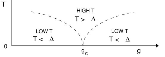
Figure 1.  : Schematic phase diagram as a function of the coupling constant of the quantum Hamiltonian $g$, and the temperature $T$. The quantum critical point is at $T=0$, $g=g_{c}$. The dashed lines indicate crossovers. There may finite temperature phase transitions in either of the two low temperature regimes. The symbol $\Delta$ represents a characteristic energy scale of the $T=0$ theory; it vanishes at $g$ approaches $g_{c}$ according to (1).

Our study will find two regimes with very different physical properties, as sketched in Fig 1:
(i) The low temperature region $k_{B}T\ll\Delta$
There are actually two regimes of this type, one on either side of $g_{c}$. Correlations in this region are similar to those of the $T=0$ ground state. The low temperature creates a small density of excitations which can sometimes have significant effects at very long scales.
(ii) The high temperature region $\Delta\ll k_{B}T$
As we are discussing universal properties of the CQFT, it is implicitly assumed that all energy scales, including $k_{B}T$, are smaller than the upper cutoff $\bar{\Lambda}$ which has been sent to infinity; so we also require that $k_{B}T\ll\bar{\Lambda}$. The thermal energy, $k_{B}T$, sets the scale for all physical phenomena in this region, and the system behaves as if it’s couplings are at the $g=g_{c}$ critical point. We shall devote much attention to the unfamiliar and unusual properties of this region. It is perhaps worth noting explicitly why the high $T$ limit of the CQFT can be non-trivial. A conventional high $T$ expansions of the lattice model ${\cal H}$ proceeds with the series

$$\mbox{Tr}e^{-{\cal H}/k_{B}T}=\mbox{Tr}1-\frac{1}{k_{B}T}\mbox{Tr}{\cal H}+\frac{1}{2(k_{B}T)^{2}}\mbox{Tr}{\cal H}^{2}+\ldots$$ (2)

The successive terms in this series are well-defined and finite because of the ultraviolet cutoffs provided by the lattice. Further, the series is well-behaved provided $T$ is larger than all other energy scales; in particular we need $k_{B}T\gg\bar{\Lambda}$. In contrast, the CQFT was defined by the limit $\bar{\Lambda}\rightarrow\infty$ at fixed $k_{B}T$, $\Delta$, and, as already stated, the high $T$ limit of the CQFT corresponds to the intermediate temperature range $\Delta\ll k_{B}T\ll\bar{\Lambda}$ of the lattice model. It is not possible to access this temperature range by an expansion as simple as (2), and more sophisticated techniques, to be discussed here, are necessary.

All of our explicit computations will be with models described by the same CQFT. This is the relativistic CQFT in $d$ spatial dimensions with imaginary time ($\tau$) action

$${\cal S}= \int_{0}^{\hbar/k_{B}T}d\tau\int d^{d}x\left\{\frac{1}{2}\left[(\partial_{\tau}\phi_{\alpha})^{2}+c^{2}(\nabla_{x}\phi_{\alpha})^{2}\right.\right.$$ (3)

$$~{}~{}~{}~{}~{}~{}~{}~{}~{}~{}~{}~{}~{}~{}~{}~{}~{}~{}~{}~{}~{}~{}~{}~{}~{}~{}~{}~{}~{}~{}~{}\left.\left.+(m_{0c}^{2}+(g-g_{c}))\phi_{\alpha}^{2}\right]+\frac{u_{0}}{4!}(\phi_{\alpha}^{2})^{2}\right\}.$$

Here $\phi_{\alpha}$ is a real scalar field, the index $\alpha=1\ldots N$ is implicitly summed over, and the action has $O(N)$ symmetry. This CQFT has a “Lorentz” invariance with $c$ the velocity of “light”, and as a result the dynamic critical exponent $z=1$. The bare “mass” term has been written as $m_{0c}^{2}+(g-g_{c})$ so that the $T=0$ quantum critical point is at $g=g_{c}$, and $u_{0}$ measures the strength of the quartic non-linearity. The action ${\cal S}$ can also be interpreted as the Gibbs weight of a classical statistical mechanics problem in $d+1$ dimensions (with the $\tau$ dimension of finite extent $\hbar/k_{B}T$); indeed it is nothing but the standard, thoroughly-studied $\phi^{4}$ theory which is the corner-stone of the well established theory of classical critical phenomena [1]. It might then appear that we can simply carry over these results to the case of the quantum-critical point, and our job is relatively straightforward. This is far from being the case. The fundamental reason is that all dynamic experimental measurements are in real time ($t$), and we are particularly interested in the long time limit $t\gg\hbar/k_{B}T$. While, in principle, information on these long-time correlations is related by analytic continuation to imaginary time correlations in the domain $0<\tau<\hbar/k_{B}T$, in practice the continuation is an ill-posed problem, and essentially impossible to carry out. In particular, it has been shown [6, 7, 8] that the operations of expansion in $\epsilon=3-d$ or $1/N$ (which are the only non-numeric tools available for analyzing ${\cal S}$), and of analytic continuation do not commute. It is essential that the theory of the dynamic and transport properties of ${\cal S}$ be formulated directly in real time, and here we shall review recent progress in this direction. It is sobering to note that there remain open questions on experimentally important observables even for the simple model ${\cal S}$, and we shall also note them here.

A central concept in our description of the dynamic properties of ${\cal S}$ is that of the phase relaxation time, $\tau_{\varphi}$. This is defined as the time over which the wave-functional of the CQFT retains phase memory. We shall find that in the regions of Fig 1

$$\tau_{\varphi} \sim \hbar/k_{B}T~{}~{}~{}~{}\mbox{in the ``High T'' region}$$

$$\tau_{\varphi} \gg \hbar/k_{B}T~{}~{}~{}~{}\mbox{in the ``Low T'' regions}$$ (4)

These relations will be shown to apply to ${\cal S}$, but are expected to be far more general. The missing constant in the first of these relations is a universal number which depends upon the precise definition of $\tau_{\varphi}$. All of the physical properties of ${\cal S}$ will show significant crossovers at times of order $\tau_{\varphi}$ which we shall describe.

2 The Ising chain in a transverse field

We will begin by obtaining exact results for the dynamic scaling functions of ${\cal S}$ for the case $d=1$, $N=1$. The quantum physics is more transparent in a lattice Hamiltonian formulation, where the properties of ${\cal S}$ are expected to be equivalent to those of the Ising chain in a transverse field (this may be shown in a manner similar to Section 3.2 which considers $N>1$). The degrees of freedom of the Ising model are spins $\sigma^{z}_{i}$ on the sites, $i$, of a chain. In addition to their usual exchange interaction $J$, there is a transverse field of strength $gJ$ which is responsible for the quantum dynamics; thus the Hamiltonian is

$$H_{I}=-J\sum_{i}\left(g\sigma^{x}_{i}+\sigma^{z}_{i}\sigma^{z}_{i+1}\right)$$ (5)

Like ${\cal S}$ for $N=1$, $H_{I}$ possesses a global $Z_{2}$ symmetry: it is invariant under a unitary transformation performed by the operator $\prod_{i}\sigma^{x}_{i}$ under which

$$\sigma^{z}_{i}\rightarrow-\sigma^{z}_{i}~{}~{}~{}~{}~{}~{}~{}~{}\sigma^{x}_{i}\rightarrow\sigma^{x}_{i}$$ (6)

Notice that this global Ising $Z_{2}$ symmetry is present in the presence of the transverse field. A longitudinal field, coupling to $\sigma^{z}$ would break the $Z_{2}$ symmetry. The action of this symmetry correctly indicates that the operator correspondence $\sigma^{z}\sim\phi$ maps the long distance correlators of ${\cal S}$ and $H_{I}$.

2.1 Limiting cases

We begin by examining the spectrum of $H_{I}$ under strong ($g\gg 1$) and weak ($g\ll 1$) coupling [9]. The analysis is relatively straightforward in these limits, and two very different physical pictures emerge. The exact solution, to be discussed later, shows that there is a critical point exactly at $g=1$, but that the qualitative properties of the ground states for $g>1$ ($g<1$) are very similar to those for $g\gg 1$ ($g\ll 1$). One of the two limiting descriptions is therefore always appropriate, and only the critical point $g=1$ has genuinely different properties.

Strong coupling $g\gg 1$

Let $\left|\uparrow\right\rangle_{i}$ and $|\downarrow\rangle_{i}$ denote the eigenstates of $\sigma^{z}_{i}$. Then $|\pm\rangle_{i}=(\left|\uparrow\right\rangle_{i}\pm|\downarrow\rangle_{i})/\sqrt{2}$ are the eigenstates of $\sigma^{x}_{i}$. Then at $g=\infty$ the ground state of $H_{I}$ is clearly determined by the transverse field term to be

$$|0\rangle=\prod_{i}|+\rangle_{i}$$ (7)

The values of $\sigma^{z}_{i}$ on different sites are totally uncorrelated in this state, and so $\langle 0|\sigma^{z}_{i}\sigma^{z}_{j}|0\rangle=\delta_{ij}$. Perturbative corrections in $1/g$ will build in correlations in $\sigma^{z}$ which increase in range at each order in $1/g$; for $g$ large enough these correlations are expected to remain short-ranged, and the $\sigma^{z}$ correlator to decay exponentially with separation. There is thus no magnetic long-range order and this state is a “quantum paramagnet”. Notice that this state is invariant under the $Z_{2}$ symmetry described above.

What about the excited states ? For $g=\infty$ these can also be listed exactly. The lowest excited states are

$$|i\rangle=|-\rangle_{i}\prod_{j\neq i}|+\rangle_{j},$$ (8)

obtained by flipping the state on site $i$ to the other eigenstate of $\sigma^{x}$. All such states are degenerate, and we will refer to them as the “single-particle” states. Similarly, the next degenerate manifold of states are the two-particle states $\left|i,j\right\rangle$, obtained by flipping the states at sites $i$ and $j$, and so on to the general $n$-particle states. To leading order in $1/g$, we can neglect the mixing between states between different particle number, and just study how the degeneracy within each manifold is lifted. For the one-particle states, the exchange term in $H_{I}$ leads only to the off-diagonal matrix element

$$\langle i|H_{I}|i+1\rangle=-J$$ (9)

which hops the ‘particle’ between nearest neighbor sites. As in the tight-binding models of solid state physics, the Hamiltonian is therefore diagonalized by going to the momentum space basis

$$|k\rangle=\frac{1}{\sqrt{N}}\sum_{i}e^{ikx_{i}}|i\rangle$$ (10)

where $N$ is the number of sites. This eigenstate has energy (we have choosen an overall constant in $H_{I}$ to make the energy of the ground state zero)

$$\varepsilon_{k}=Jg\left(2-(2/g)\cos ka+{\cal O}(1/g^{2})\right)$$ (11)

where $a$ is the lattice spacing. The lowest energy one-particle state is therefore at $\varepsilon_{0}=2g-2J$

Now consider the two-particle states. As long as the two particles are well separated from each other, the eigenstate is formed simply by taking the tensor product of two single particle eigenstates. However these particles will collide, which will be described by a $S$ matrix. If we exclude the possibility of two-particle bound states (which do not occur here), the total energy of the state is determined by the configuration where the particles are well separated, and is simply the sum of the single particle energies. Thus the energy of a two-particle state with total momentum $k$ is given by $E_{k}=\varepsilon_{k_{1}}+\varepsilon_{k_{2}}$ where $k=k_{1}+k_{2}$. Notice that for a fixed $k$, there is still an arbitrariness in the single particle momenta $k_{1,2}$ and so the total energy $E_{k}$ can take a range of values. There is thus no definite energy momentum relation, and we have instead a ‘two-particle continuum’. It should be clear, however, that the lowest energy two-particle state in the infinite system (its “threshold”) is at $2\varepsilon_{0}$. Similar considerations apply to the $n$-particle continua, which have thresholds at $n\varepsilon_{0}$.

At next order in $1/g$ we have to account for the mixing between states with differing numbers of particles. Non-zero matrix elements like

$$\langle 0|H_{I}|i,i+1\rangle=-J$$ (12)

lead to a coupling between $n$ and $n+2$ particle states. It is clear that these will renormalize the one-particle energies $\varepsilon_{k}$. However qualitative features of the spectrum will not change, and we will still have renormalized one-particle states with a definite energy-momentum relationship, and renormalized $n\geq 2$ particle continua with thresholds at $n\varepsilon_{0}$.

The same expansion in powers of $1/g$ can also be used to compute the two-particle $S$ matrix. If we consider the collision of two-particles with small momenta $p$ and $p^{\prime}$, then by conservation of energy and momentum there can only be two particles in the final state, and the momenta of these particles remains $p$ and $p^{\prime}$. An elementary calculation to order $1/g$ shows then that

$$S_{pp^{\prime}}=-1.$$ (13)

It can be shown that this result holds in limit of small $p$, $p^{\prime}$ to all orders in $1/g$ for a large class of models like $H_{I}$ with further neighbor exchange. The particles under consideration, being simple spin flips, are evidently bosons which experience a short-range repulsive potential. In $d=1$ any weak repulsive potential appears arbitrarily strong in the limit of low velocities, and leads to the ‘unitarity limit’ phase shift of $\pi$, which is responsible for (13). For the particular nearest neighbor model $H_{I}$, it can be shown that there is no particle production in collisions at any incoming momenta $p$, $p^{\prime}$, and that (13) holds to all orders in $1/g$ for all $p$, $p^{\prime}$. This will be shown and exploited in Section 2.2.

The spectrum described above has simple, but important, consequences for the dynamic spin susceptibility $\chi(k,i\omega_{n})$. This is defined in imaginary time as the Fourier transform into momentum and frequency of the $\sigma^{z}$ correlator:

$$\chi(k,i\omega_{n})=\int_{0}^{1/T}d\tau\int dx\left\langle\sigma^{z}(x,i\tau)\sigma^{z}(0,0)\right\rangle e^{i(kx-\omega_{n}\tau)}$$ (14)

Its spectral density $\chi^{\prime\prime}(p,\omega)$ is the imaginary part of the real frequency $\chi(k,\omega)$, and it given by

$$\chi^{\prime\prime}(k,\omega)=\pi\sum_{a}|\left\langle 0|\sigma^{z}(k)|a\right\rangle|^{2}\delta(\omega-E_{a})$$ (15)

where the sum over $a$ extends over all the eigenstates of $H_{I}$ with energy $E_{a}$. The eigenstates and energies described above allow us to simply deduce the qualitative form of $\chi^{\prime\prime}(p,\omega)$ which is sketched in Fig 2.

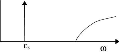
Figure 2.  : Schematic of the spectral density $\chi^{\prime\prime}(k,\omega)$ of $H_{I}$ as a function of $\omega$ at $T=0$ and a small $k$. There is a quasiparticle delta function at $\omega=\varepsilon_{k}$, and a three-particle continuum at higher frequencies.

The operator $\sigma^{z}$ flips the state at a single site, and so the matrix element in (15) is non-zero for the single particle states: only the state with momentum $p$ will contribute, and so there is an infinitely sharp delta function contribution to $\chi^{\prime\prime}(k,\omega)\sim\delta(\omega-\varepsilon_{k})$. This delta function is the “quasiparticle peak” and its co-efficient is the quasiparticle amplitude. At $g=\infty$ this quasiparticle peak is the entire spectral density, but for smaller $g$ the quasiparticle amplitude decreases and the multiparticle states also contribute to the spectral density. The mixing between the one and three particle states discussed above, means that the next contribution to $\chi^{\prime\prime}(p,\omega)$ occurs above the 3 particle threshold $\omega>3\varepsilon_{0}$; because there are a continuum of such states, their contribution is no longer a delta function, but a smooth function of omega (apart from a threshold singularity), as shown in Fig 2. Similarly there are continua above higher odd number particle thresholds; only states with odd numbers of particles contribute because the matrix element in (15) vanishes for even numbers of particles.

Weak coupling $g\ll 1$

Now the energy is dominated by the exchange term. There are two degenerate ground states at $g=0$ with the spins either all up or down (in eigenstates of $\sigma^{z}$):

$$\left|\uparrow\right\rangle=\prod_{i}|\uparrow\rangle_{i}~{}~{}~{}~{}~{}~{}~{}\left|\downarrow\right\rangle=\prod_{i}\left|\downarrow\right\rangle_{i}$$ (16)

Turning on a small $g$ will mix in a small fraction of spins of the opposite orientation, but the degeneracy will survive as the two states are related to each other by the global $Z_{2}$ symmetry noted above (6). A thermodynamic system will always choose one or the other of the states as its ground states (which may be preferred by some infinitesimal external perturbation), and hence the $Z_{2}$ symmetry will be spontaneously broken. The correlations of the magnetization $\sigma^{z}$ have an infinite range in either state as

$$\lim_{|x|\rightarrow\infty}\left\langle\sigma^{z}(x,0)\sigma^{z}(0,0)\right\rangle=N_{0}^{2}\neq 0$$ (17)

The quantity $N_{0}$ is the spontaneous magnetization, and equals $\langle\sigma^{z}\rangle$ in either of the two ground states. All of the statements made in this paragraph clearly hold for $g=0$, and will hold for some $g>0$ provided the perturbation theory in $g$ has a non-zero radius of convergence. The exact solution of the model to be discussed later will verify that this is indeed the case.

The excited states can be described in terms of an elementary domain wall (or kink) excitation. For instance the state

$$\cdots\left|\uparrow\right\rangle_{i}\left|\uparrow\right\rangle_{i+1}\left|\downarrow\right\rangle_{i+2}\left|\downarrow\right\rangle_{i+3}\left|\downarrow\right\rangle_{i+4}\left|\uparrow\right\rangle_{i+5}\left|\uparrow\right\rangle_{i+6}\cdots$$

has domain walls, or nearest neighbor pairs of antiparallel spins, between sites $i+1$, $i+2$ and sites $i+4$, $i+5$. At $g=0$ the energy of such a state is clearly $2J\times$number of domain walls. The consequences of a small non-zero $g$ are now very similar to those due to $1/g$ corrections in the complementary large $g$ limit: the domain walls become “particles” which can hop and form momentum eigenstates with excitation energy

$$\varepsilon_{k}=J\left(2-2g\cos(ka)+{\cal O}(g^{2})\right).$$ (18)

The spectrum can be interpreted in terms $n$-particle scattering states, although it must be emphasized that the interpretation of the particle is now very different from that in the large $g$ limit. Again, the perturbation theory in $g$ only mixes states which differ by even numbers of particles, although now the matrix element in (15) is non-zero only for states $a$ with an even number of particles; these assertions can easily be checked to hold in a perturbation theory in $g$. So $\chi^{\prime\prime}(p,\omega)$ will now have a pole at $p=0$, $\omega=0^{+}$, from the term in (15) where $a=$ one of the ground states, indicating the presence of long-range order. Further, there is now no single particle contribution, and the first finite $\omega$ spectral density is the continuum above the two particle threshold. The absence of a single particle delta function in this case is a very special feature of the $d=1$, $N=1$ model, and is not expected to hold in higher $d$.

The $S$ matrix for the collision of two domain walls can now be computed in a perturbation theory in $g$, and as in the strong-coupling $1/g$ expansion, we find that there is no particle production, and $S_{pp^{\prime}}=-1$ to all orders in $g$.

2.2 Exact spectrum and continuum theory

The qualitative considerations of the previous section are quite useful in developing an intuitive physical picture. We will now take a different route, and set up a formalism that will eventually lead to an exact determination of many physical correlators; these results will vindicate the approximate methods for $g>1$, $g<1$, and also provide an understanding of the novel physics at $g=1$.

The central idea is the application of the Jordan-Wigner transformation [10, 11]. We map the $|+\rangle$, $|-\rangle$ states on each site to the Fock space of spinless fermions which can have occupation numbers $0,1$ on each site. The operator representation of the mapping is

$$\sigma^{x}_{i} = 1-2c_{i}^{\dagger}c_{i}$$

$$\sigma^{z}_{i} = (-1/2)\prod_{j<i}\left(1-2c_{j}^{\dagger}c_{j}\right)(c_{i}+c_{i}^{\dagger})$$ (19)

where $c_{i}$ is the annihilation operator for the fermion at site $i$. Inserting (19) into $H_{I}$ we find that the resulting Hamiltonian is quadratic in the fermions

$$H_{I}=-J\sum_{i}\left(c_{i}^{\dagger}c_{i+1}+c_{i+1}^{\dagger}c_{i}+c_{i}^{\dagger}c_{i+1}^{\dagger}+c_{i+1}c_{i}-2gc_{i}^{\dagger}c_{i}-g\right).$$ (20)

This Hamiltonian can be diagonalized in momentum space by a Bogoliubov transformation. The fermionic quasiparticle operators are $\gamma_{k}$ ($-\pi/a<k<\pi/a$) and the diagonal form of $H_{I}$ is

$$H_{I}=\sum_{k}\varepsilon_{k}(\gamma_{k}^{\dagger}\gamma_{k}-1/2)$$ (21)

where

$$\varepsilon_{k}=2J\left(1+g^{2}-2g\cos(ka)\right)^{1/2}$$ (22)

is the single particle energy. As $\varepsilon_{k}\geq 0$, the ground state, $|0\rangle$, of $H_{I}$ has has no $\gamma$ fermions and therefore satisfies $\gamma_{k}|0\rangle=0$ for all $k$. The excited states are created by occupying the single particle states; they can clearly be classified by the total number of occupied states, and a $n$-particle state has the from $\gamma_{k_{1}}^{\dagger}\gamma_{k_{2}}^{\dagger}\cdots\gamma_{k_{n}}^{\dagger}|0\rangle$, with all the $k_{i}$ distinct.

The above structure of the spectrum confirms the approximate considerations of Section 2.1. We have now found that the particles are in fact free fermions, and two fermions will not scatter even when they are close to each other; alternatively they can be considered as hard-core bosons which have an $S$ matrix which does not allow particle production, and which equals $-1$ at all momenta. We shall find it much more useful to take the latter point of view, as the bosonic particles have a simple, local, interpretation in terms of the underlying spin excitations: for $g\gg 1$ the bosons are simply spins oriented in the $|-\rangle$ direction, while for $g\ll 1$ they are domain walls between the two ground states. The fermionic representation is useful for certain technical manipulation, but the bosonic point of view is much more useful for making physical arguments, as we shall see below.

The excitation energy $\varepsilon_{k}$ in (22) is non-zero and positive for all $k$ provided $g\neq 1$. The energy gap, or the minimum excitation energy is always at $k=0$, and equals $2J|1-g|$. This gap vanishes at $g=1$, and it is natural to expect that $g=g_{c}=1$ is the phase boundary between the two qualitatively different phases discussed in Section 2.1. Precisely at $g=1$, fermions with low momenta can carry arbitrarily low energy, and therefore must dominate the low temperature properties. These properties suggest that the state at $g=1$ is critical, and there is a CQFT which describes the critical properties in its vicinity. As the important excitations are near $k=0$, we define the continuum Fermi field

$$\Psi(x_{i})=\frac{1}{\sqrt{a}}c_{i}$$ (23)

We express $H_{I}$ in terms of $\Psi$, and expand in spatial gradients. This gives the fermionic Lagrangean of the CQFT believed to be equivalent to ${\cal S}$ for $d=1$, $N=1$:

$${\cal L}_{I}=-\Psi^{\dagger}\frac{\partial\Psi~{}{\dagger}}{\partial\tau}+\frac{c}{2}\left(\Psi^{\dagger}\frac{\partial\Psi}{\partial x}-\Psi\frac{\partial\Psi}{\partial x}\right)+\Delta\Psi^{\dagger}\Psi$$ (24)

The field $\Psi$ is now implicitly assumed to be a function of space and imaginary time ($\tau$). The coupling constants in (24) are given for $H_{I}$ by

$$\Delta=2J(1-g)~{}~{}~{}~{}~{}~{}~{}~{}c=2Ja.$$ (25)

However, the relations (25) are very specific to the solvable model $H_{I}$. For more complicated, non-solvable, Ising models which have a similar naive continuum limit (e.g. models with second neighbor exchange), the values of $\Delta$ and $c$ appearing in the continuum quantum field theory cannot be determined exactly. Indeed $\Delta$ and $c$ are parameters which depend upon details of the microscopic Hamiltonian, i.e. they have a non-universal dependence upon a coupling constant like $g$, as can be checked by a simple estimate of perturbative fluctuation corrections due to irrelevant operators.

Comparing the dependence of $\Delta$ on $g$ in (25) with (1) we conclude that the exponent $z\nu=1$. Further at the critical point $\Delta=0$, the excitation energy $\varepsilon_{k}\sim k$, which fixes the dynamic critical exponent $z=1$.

The continuum theory ${\cal L}_{I}$ can be diagonalized much like the lattice model $H_{I}$, and the excitation energy now takes a “relativistic” form

$$\varepsilon_{k}=\left(\Delta^{2}+c^{2}k^{2}\right)^{1/2}$$ (26)

which shows that $|\Delta|$ is the $T=0$ energy gap (we will choose the sign of $\Delta$ to be different on the two sides of the critical value of $g$), and $c$ is the velocity of the excitations, both measurable quantities. The form of $\varepsilon_{k}$ correctly suggests that ${\cal L}_{I}$ is invariant under Lorentz transformations. This can be made explicit by writing the complex Grassman field $\Psi$ in terms of two real Grassman fields, when the action becomes what is known as the field theory of Majorana fermions of mass $\Delta/c^{2}$ [12]; we will not explicitly display this here.

While the continuum field $\Psi$ has no direct physical interpretation, its correlators are easily computed at all $g$, including the critical point $g=1$. To gain some insight about this point, we explicitly display a certain $\Delta=0$ two-point correlator for $T\geq 0$. We find for imaginary time $\tau>0$

$$\left\langle\Psi(x,i\tau)\Psi^{\dagger}(0,0)\right\rangle=\frac{1}{2}\int_{-\infty}^{\infty}\frac{dk}{2\pi}\frac{e^{ikx}}{e^{c|k|/T}+1}\left(e^{c|k|(1/T-\tau)}+e^{c|k|\tau}\right)$$

$$~{}~{}~{}~{}~{}~{}~{}~{}~{}~{}=\left(\frac{T}{4c}\right)\left(\frac{1}{\sin(\pi T(\tau-ix/c))}+\frac{1}{\sin(\pi T(\tau+ix/c))}\right).$$ (27)

We are now using units in which $\hbar=k_{B}=1$, and will continue to do so in the remainder of the paper. At $T=0$, (27) simplifies to

$$\left\langle\Psi(x,\tau)\Psi^{\dagger}(0,0)\right\rangle=\frac{1}{4\pi}\left(\frac{1}{c\tau-ix}+\frac{1}{c\tau+ix}\right),$$ (28)

when we notice that the transformation

$$c\tau\pm ix\rightarrow\frac{c}{\pi T}\sin\left(\frac{\pi T}{c}(c\tau\pm ix)\right)$$ (29)

connects the $T=0$ and $T>0$ results. This transformation is actually a very general property of the critical point, and connects all $T=0$ and $T>0$ correlators; it is a consequence of the conformal invariance [13] of ${\cal L}_{I}$ at $\Delta=0$. We will use (29) in an important way later.

Correlators of $\sigma^{x}$ can be constructed out of those of simple bilinears of the fermion operators, and we will not display them explicitly. More interesting, however, are the correlators of the order parameter $\sigma^{z}\sim\phi$. Computing just the equal time two-point correlator, or even simply the value of its scaling dimension, $\mbox{dim}[\sigma^{z}]$, involves a rather lengthy and involved computation, which will not be discussed here. Rather, in the next section, we will quote a recently obtained technical result, and then proceed to obtain dynamic correlators of $\sigma^{z}$ by simple physical arguments.

2.3 Finite temperature crossovers

The purpose of this section is to describe the dynamics of the order parameter in the different regions of the $T>0$ phase diagram sketched in Fig 3; this diagram follows from the considerations in Section 1, the expression for $\Delta$ in (25), and computations to be described below.

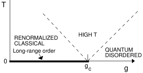
Figure 3.  : Finite $T$ phase diagram of the $d=1$ quantum Ising model, $H_{I}$, as a function of the coupling $g$ and temperature $T$. There is a quantum phase transition at $T=0$ $g=g_{c}$ with exponents $z=1$, $\nu=1$. Long-range order ($N_{0}=\langle\sigma_{z}\rangle\neq 0$) is present only for $T=0$ and $g<g_{c}$. There is an energy gap above the ground state for all $g\neq g_{c}$. We use an energy scale $\Delta\sim g_{c}-g$ such that the energy gap is $|\Delta|$. The dashed lines are crossovers at $|\Delta|\sim T$. A very similar phase diagram also applies to the $d=2$ $O(3)$ quantum rotor model discussed in Section 3.4. In this case there is no energy gap for $g<g_{c}$, and the spin-stiffness $\rho_{s}$ is used as the energy scale to characterize the ground state. There is an energy gap $\Delta$ for $g>g_{c}$. These energies vanish as $\rho_{s}\sim(g_{c}-g)^{z\nu}$, $\Delta\sim(g-g_{c})^{z\nu}$ with $z=1$, $\nu\approx 0.7$, and so the crossover phase boundaries at $T\sim|g-g_{c}|^{z\nu}$ will not be linear.

As noted earlier, here we will quote just one technical result on the equal-time two-point correlator of $\sigma^{z}$ for $T>0$ which was obtained [14, 15, 16] using the fermion mapping. We will then show, following the recent work of Ref. [17], that unequal-time, $T>0$, correlations can be obtained by simple physical arguments that rely on the bosonic picture of the excitations developed in Section 2.1 using the large and small $g$ expansions. It is worth noting that very sophisticated methods [18, 19] relying on the fermion mapping have not so far succeeded in obtaining any explicit results for unequal time correlations for $T>0$ (there are some results [20] on time-dependent correlators at $T=\infty$ which are non-universal and unrelated to the CQFT of interest here),

The equal-time, long-distance result we need is [16]

$$\left\langle\sigma^{z}(|x|\rightarrow\infty,t=0)\sigma^{z}(0,0)\right\rangle=ZT^{1/4}G_{I}(\Delta/T)\exp\left(-\frac{T|x|}{c}F_{I}(\Delta/T)\right)$$ (30)

where $t$ is real time, $Z$ is non-universal constant, and $F_{I}(s)$ and $G_{I}(s)$ are universal scaling functions. The crucial property of (30) is the prefactor of $T^{1/4}$. As $T$ is an energy which scales as inverse time, and the dynamic exponent $z=1$, this allows us to conclude that the scaling dimension of $\sigma^{z}$ ($\phi$) is

$$\mbox{dim}[\sigma^{z}]=1/8.$$ (31)

From (30), we can also define the correlation length $\xi$ which obeys

$$\xi^{-1}=\frac{T}{c}F_{I}\left(\frac{\Delta}{T}\right)$$ (32)

The exact, self-contained expression for the universal function $F_{I}$ is [16]

$$F_{I}(s)=\frac{1}{\pi}\int_{0}^{\infty}dy\ln\coth\frac{(y^{2}+s^{2})^{1/2}}{2}+|s|\theta(-s).$$ (33)

The $s>0$ ($s<0$) portion of $F_{I}$ describes the ordered (disordered) side. Despite appearances, the function $F_{I}(s)$ is smooth as a function of $s$ for all real $s$, and is analytic at $s=0$. The analyticity at $s=0$ is required by the absence of any thermodynamic singularity at finite $T$ for $\Delta=0$. This is a key property, which was in fact used to obtain the answer in (33). The exact expression for the function $G_{I}(s)$ is also known

$$\ln G_{I}(s)=\int_{s}^{1}\frac{dy}{y}\left[\left(\frac{dF_{I}(y)}{dy}\right)^{2}-\frac{1}{4}\right]+\int_{1}^{\infty}\frac{dy}{y}\left(\frac{dF_{I}(y)}{dy}\right)^{2},$$ (34)

and its analyticity at $s=0$ follows from that of $F_{I}$. For the solvable model $H_{I}$, we chose the overall normalization of $G_{I}$ such that $Z=J^{-1/4}$. In general, the value of $Z$ is set by relating it to an observable, as we will show below. Also note that $Z$ has no dependence on $\Delta$, and is therefore non-singular at the quantum critical point.

Armed with the above knowledge, we can write down the full scaling form for the time-dependent $\sigma^{z}$ correlator, which applies to the lattice model in the limits $\bar{\Lambda}\sim J\rightarrow\infty$, $a\rightarrow 0$ at fixed $\Delta$, $c$ and $T$

$$\left\langle\sigma^{z}(x,t)\sigma^{z}(0,0)\right\rangle=ZT^{1/4}\Phi_{I}\left(\frac{Tx}{c},T\tau,\frac{\Delta}{T}\right)$$ (35)

where $\Phi_{I}$ is a universal function which is analytic as a function of its third argument $s=\Delta/T$ on the real $s$ axis. The result (30) obviously specifies $\Phi_{I}$ for large $Tx/c$ and $t=0$.

The following subsections will describe the unequal-time form of $\Phi_{I}$ in the limiting regions of Fig 3: they are associated with the limits $s\rightarrow\infty$ (renormalized classical), $s\rightarrow-\infty$ (quantum disordered), and $s=0$ (high $T$) of $F_{I}$, $G_{I}$ which will also be noted below.

Low $T$ on the ordered side, $\Delta>0$, $T\ll\Delta$

This is the “renormalized classical” [21] region of Fig 3, and the reasons for this name will become clear below.

Assuming that it is valid to interchange the limits $T\rightarrow 0$ and $x\rightarrow\infty$ in (30), we can use the limiting values $F_{I}(\infty)=0$, $G_{I}(s\rightarrow\infty)=s^{1/4}$ to deduce that (recall (17)):

$$N_{0}^{2}\equiv\lim_{|x|\rightarrow\infty}\left\langle\sigma^{z}(x,0)\sigma^{z}(0,0)\right\rangle=Z\Delta^{1/4}~{}~{}~{}~{}~{}\mbox{at $T=0$.}$$ (36)

Thus, as claimed earlier, there is long-range order in the $g<1$ ground state of $H_{I}$, with the order parameter $N_{0}=\langle\sigma^{z}\rangle=Z^{1/2}\Delta^{1/8}$ (this relates the value of $Z$ to a physical observable). For small $T\ll\Delta$, we obtain from the large $s$ behavior of $F_{I}(s)$ (see (33)) that

$$\left\langle\sigma^{z}(x,0)\sigma^{z}(0,0)\right\rangle=N_{0}^{2}e^{-|x|/\xi_{c}}~{}~{}~{}\mbox{large $|x|$},$$ (37)

where the correlation length

$$\xi_{c}^{-1}=\left(\frac{2\Delta T}{\pi c^{2}}\right)^{1/2}e^{-\Delta/T}.$$ (38)

is finite at any non-zero $T$, showing that long-range order is present only precisely at $T=0$. We have put a subscript $c$ on the correlation length to emphasize that the system is expected to behave classically in this low temperature region [16]. The excitations above the ground states consists of particles (the kinks and anti-kinks of Section 2.1) whose mean separation ($\sim\xi_{c}$) is much larger than their de Broglie wavelengths ($\sim(c^{2}/\Delta T)^{1/2}$, as the mass of these particles = $\Delta/c^{2}$), which is precisely the canonical condition for the applicability of classical physics. It is also reassuring to note that (37) is precisely the form of equal-time correlations in the classical Ising model at low $T$. The prefactor $N_{0}^{2}$ is the true ground state magnetization including the effects of quantum fluctuations, and this is the reason for the adjective “renormalized” in the name for this region.

We now show, following Ref [17], that it is possible to give a simple physical interpretation for the precise value of $\xi_{c}$ in (38). The energy of a domain wall with a small momentum $k$ is $\Delta+c^{2}k^{2}/2\Delta$, and therefore classical Boltzmann statistics tells us that their density, $\rho$, is

$$\rho=\int\frac{dk}{2\pi}e^{-(\Delta+c^{2}k^{2}/2\Delta)/T}=\left(\frac{T\Delta}{2\pi c^{2}}\right)^{1/2}e^{-\Delta/T}.$$ (39)

Comparing with (38), we see that $\xi_{c}=1/2\rho$. We now show that this result follows immediately if we assume that the domain walls are classical point particles, which are distributed independently with a density $\rho$. Consider a system of size $L\gg|x|$, and let it contain $M$ thermally excited particles; then $\rho=M/L$. Let $q$ be the probability that a given particle will be between $0$ and $x$. Clearly, $q=|x|/L$. The probability that a given set of $j$ particles are the only ones between 0 and $x$ is then $q^{j}(1-q)^{M-j}$: as each particle reverses the orientation of the ground state, in this case $\sigma^{z}(x,0)\sigma^{z}(0,0)=N_{0}^{2}(-1)^{j}$. Summing over all possibilities we have

$$\langle\sigma^{z}(x,0)\sigma^{z}(0,0)\rangle = N_{0}^{2}\sum_{j=0}^{M}(-1)^{k}q^{j}(1-q)^{M-j}\frac{M!}{j!(M-j)!}$$ (40)

$$= N_{0}^{2}(1-2q)^{N}\approx N_{0}^{2}e^{-2qM}=N_{0}^{2}e^{-2\rho|x|},$$

thus establishing the desired result.

This classical picture can also be extended to compute unequal time correlations [17]. Let us explicitly consider the form of the correlation function needed

$$\langle\sigma^{z}(x,t)\sigma^{z}(0,0)\rangle=\mbox{Tr}\left(e^{-H_{I}/T}e^{iH_{I}t}\sigma^{z}_{i}e^{-iH_{I}t}\sigma^{z}_{0}\right)/Z,$$ (41)

where $Z=\mbox{Tr}e^{-H_{I}/T}$. We evaluate it in the double-time (‘Keldysh’) path integral formalism [22]. The path integral is over a set of trajectories moving forward in time, representing the operator $e^{-iH_{I}t}$, and a second set moving backwards in time, corresponding to the action of $e^{iH_{I}t}$. In the semiclassical limit, stationary phase is achieved when the backward paths are simply the time reverse of the forward paths, and both sets are the classical trajectories. An example of a set of paths is shown in Fig 4.

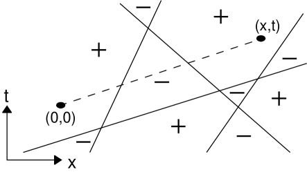
Figure 4.  : A typical semiclassical contribution to the double time path integral for $\langle\sigma^{z}(x,t)\sigma^{z}(0,0)\rangle$. Full lines are thermally excited particles which propagate forward and backward in time. The $\pm$ signs are significant only for $g<1$ and denote the orientation of the order parameter. For $g>1$, the dashed line is a particle propagating only forward in time from $(0,0)$ to $(x,t)$.

Now observe that (i) the classical trajectories remain straight lines across collisions because the momenta before and after the collision are the same in one dimension; (ii) for each collision, the amplitude for the path acquires a phase $S_{pp^{\prime}}$ along the forward path and its complex conjugate along the backward path: the net factor for the collision is therefore $|S_{pp^{\prime}}|^{2}=1$. These two facts imply that the trajectories are simply independently distributed straight lines, placed with a uniform density $\rho$ along the $x$ axis, with an inverse slope

$$v_{k}\equiv\frac{d\varepsilon_{k}}{dk},$$ (42)

and with their momenta chosen with the Boltzmann probability density $e^{-\varepsilon_{k}/T}/\rho$ (Fig 4).

Computing dynamic correlators is now an exercise in classical probabilities. The value of $\sigma^{z}(0,0)\sigma^{z}(x,t)$ is the square of the magnetization renormalized by quantum fluctuations ($N_{0}^{2}$), times $(-1)$ if the number of trajectories intersecting the dashed line in Fig. 4 is odd. This precisely the computation carried out above for the equal time correlations, but now it is easy to see from Fig 4 that for particles with velocity $v_{k}$

$$q=\frac{|x-v_{k}t|}{L}$$ (43)

Averaging over velocities, and then proceeding as in (40) we obtain one of our central results [17, 23]

$$\langle\sigma^{z}(x,t)\sigma^{z}(0,0)\rangle=N_{0}^{2}\exp\left(-\int\frac{dk}{\pi}e^{-\varepsilon_{k}/T}\left|x-v_{k}t\right|\right).$$ (44)

Notice that the equal-time correlator is $N_{0}^{2}e^{-|x|/\xi_{c}}$ as before, and the equal-space correlator decays exponentially in time as $N_{0}^{2}e^{-|t|/\tau_{c}}$, but the general behavior is more complicated. The classical relaxation time $\tau_{c}$ is a central quantity; remarkably, we find from (44) that the correlation time, $\tau_{c}$, is independent of the functional form of $\varepsilon_{k}$ and depends only on the gap:

$$\tau_{c}=\frac{\pi\hbar}{2k_{B}T}e^{\Delta/k_{B}T},$$ (45)

where we have momentarily inserted the fundamental constants $\hbar$, $k_{B}$ to emphasize the universality of the prefactor. As $\tau_{c}$ is also the time over which the phase coherence of the ground state is lost, we may identify the phase relaxation time of Section 1 as $\tau_{\varphi}=\tau_{c}$.

In the limit $T\ll\Delta$ we are now able to completely specify the form of the scaling function $\Phi_{I}$ in (35). We find that $\Phi_{I}$ collapses into a reduced scaling function $\Phi_{Ic}$ which is determined by classical thermal physics. In particular we have

$$\left\langle\sigma^{z}(x,t)\sigma^{z}(0,0)\right\rangle=N_{0}^{2}\Phi_{Ic}\left(\frac{x}{\xi_{c}},\frac{t}{\tau_{c}}\right),$$ (46)

with

$$\ln\Phi_{Ic}(\bar{x},\bar{t})=-\bar{x}~{}\mbox{erf}\left({\bar{x}\over\bar{t}\sqrt{\pi}}\right)-\bar{t}e^{-\bar{x}^{2}/(\pi\bar{t}^{2})}.$$ (47)

Notice that the characteristic time $\tau_{c}$ and length $\xi_{c}$ both diverge as $\sim e^{\Delta/T}$, and so we can define an effective classical dynamic exponent $z_{c}=1$ (there is no fundamental reason why $z_{c}$ and $z$ should have the same value). Classical scaling forms like (46) have been discussed earlier [16], but it was incorrectly conjectured that the scaling functions would be those of the Glauber model [24] (which has $z_{c}=2$); Glauber dynamics does not conserve total energy and momentum, and these conservation laws have played a crucial role in the kinematic constraints on particle collisions.

All of the results above have been compared with exact numerical computations and the agreement is essentially perfect [17], giving us confidence in the physical approach used to understand dynamic properties at $T>0$.

Low $T$ on the disordered side, $\Delta<0$, $T\ll|\Delta|$

This is the “quantum disordered” region of Fig 3.

Now we need to take the $s\rightarrow-\infty$ limit of the functions $F_{I}(s)$, $G_{I}(s)$; from these limits we find

$$\left\langle\sigma^{z}(x,0)\sigma^{z}(0,0)\right\rangle=\frac{ZT}{|\Delta|^{3/4}}e^{-|r|/\xi}~{},~{}\mbox{$|x|\rightarrow\infty$ at fixed $0<T\ll|\Delta|$},$$ (48)

with the correlation length $\xi$ given by

$$\xi^{-1}=\frac{|\Delta|}{c}+\left(\frac{2|\Delta|T}{\pi c^{2}}\right)^{1/2}e^{-|\Delta|/T}$$ (49)

So correlations decay exponentially on a scale $\sim c/|\Delta|$, and there is no long-range order. The equal time correlations at $T=0$ behave in a similar manner, although the limits $T\rightarrow 0$ and $|x|\rightarrow\infty$ do not commute for the prefactor of the exponential decay. The $T=0$ result is determined by the form-factor expansion technique [25], which we will not discuss here; it yields [26, 19]

$$\left\langle\sigma^{z}(x,0)\sigma^{z}(0,0)\right\rangle=Z|\Delta|^{1/4}\left(\frac{c}{2\pi|\Delta||x|}\right)^{1/2}e^{-\Delta|x|/c}~{},~{}\mbox{$|x|\rightarrow\infty$ at $T=0$}.$$ (50)

The form factor expansion also yields the $T=0$ dynamic susceptibility (defined in (14)). The leading term is in fact precisely the quasiparticle pole at energy $\varepsilon_{k}=(c^{2}k^{2}+\Delta^{2})^{1/2}$ that was argued to exist in this phase in Section 2.1. We have

$$\chi(k,\omega)=\frac{2cZ|\Delta|^{1/4}}{c^{2}k^{2}+\Delta^{2}-(\omega+i\delta)^{2}}+\ldots~{}~{},~{}\mbox{$T=0$}$$ (51)

where $\delta$ is a positive infinitesimal. The imaginary part of this gives the delta function sketched in Fig 2; the continuum of excitations above the three particle threshold come from higher order terms in the form factor expansion, and are represented by the ellipsis in (51). It can now be checked that the Fourier transform of (51) yields the leading term (50) in the equal time correlation function.

The result (51) shows that the quasiparticle residue is $2Z\Delta^{1/4}$ (this is another relation between $Z$ and a physical measurable, and along with (36), it implies a relationship between the values of the residue and $N_{0}$ as we approach the critical point from either side). The residue vanishes at the critical point $\Delta=0$, where the quasiparticle picture breaks down, and we will have a completely different structure of excitations.

The above is an essentially complete description of the correlations and excitations of the quantum paramagnetic ground state. We now turn to the dynamic properties at $T>0$. At nonzero $T$, there will be a small density of quasi-particle excitations which will behave classically for the same reasons as in Section 2.3: their mean spacing is much larger than their de Broglie wavelength. The collisions of these thermally excited quasi-particles will lead to a broadening of the delta function pole in (51): the form of this broadening can be computed exactly in the limit $T\ll|\Delta|$ using a semiclassical approach similar to that employed for the ordered side [17]. The argument again employs a semiclassical path-integral approach to evaluating the correlator in (41). The key observation now is that we may consider the operator $\sigma^{z}$ to be given by

$$\sigma^{z}(x,t)=2Z|\Delta|^{1/4}(\psi(x,t)+\psi^{\dagger}(x,t))+\ldots$$ (52)

where $\psi^{\dagger}$ is the operator which creates a single particle excitation from the ground state, and the ellipsis represent multi-particle creation/annihilation terms which are subdominant in the long time limit. This representation may also be understood from the $g\gg 1$ picture discussed earlier, in which the single-particle excitations where $|-\rangle$ spins: the $\sigma^{z}$ operator flips spins between the $\pm x$ directions, and therefore creates and annihilates quasiparticles.

The computation of the nonzero $T$ relaxation is best done in real space and time, so let us first write down the $T=0$ correlations in this representation. We define $K(x,t)$ to be $T=0$ correlator of the order parameter:

$$K(x,t) \equiv \langle\sigma^{z}(x,t)\sigma^{z}(0,0)\rangle_{T=0}$$ (53)

$$= \int\frac{dk}{2\pi}\frac{cZ|\Delta|^{1/4}}{\varepsilon_{k}}e^{ikx-\varepsilon_{k}t}$$

$$= \frac{Z|\Delta|^{1/4}}{\pi}K_{0}(|\Delta|(x^{2}-c^{2}t^{2})^{1/2}/c)$$

where $K_{0}$ is the modified Bessel function. This result is just the Fourier transform of (51. Note that for $t>|x|/c$, the Bessel function has imaginary argument and is therefore complex and oscillatory.

Now we consider the $T\neq 0$ evaluation of (41) in the semiclassical path-integral approach [17]. A typical set of paths contributing to the Keldysh path integral is still given by Fig 4, but its physical interpretation is now very different. The dashed line now represents the trajectory of a particle created at $(0,0)$ and annihilated at $(x,t)$, and $\pm$ signs in the domains should be ignored. In the absence of any other particles this dashed line would contribute $K(x,t)$ to $\langle\sigma^{z}(x,t)\sigma^{z}(0,0)\rangle$. The scattering off the background particles (the full lines in Fig 4) introduces factors of the $S$-matrix element $S_{pp^{\prime}}$; as the dashed line only propagates forward in time, the $S$-matrix elements for collisions between the dashed and full lines (and only these) are not neutralized by a complex conjugate partner. Using the low momentum value $S_{pp^{\prime}}=-1$, we see that the contribution to $\langle\sigma^{z}(x,t)\sigma^{z}(0,0)\rangle$ equals $(-1)^{n_{\ell}}K(x,t)$ where $n_{\ell}$ is the number of full lines intersecting the dashed line. The $(-1)^{n_{\ell}}$ is precisely the term that appeared in the renormalized-classical, although for very different reasons. We can carry out the averaging over all trajectories as before, and obtain one of our main results [17]

$$\langle\sigma^{z}(x,t)\sigma^{z}(0,0)\rangle=K(x,t)\exp\left(-\int\frac{dk}{\pi}e^{-\varepsilon_{k}/T}\left|x-v_{k}t\right|\right),$$ (54)

where $K(x,t)$ is given by Eq. (53).

The result (54) clearly displays the separation in scales at which quantum and thermal effects act. Quantum fluctuations determine the oscillatory, complex function $K(x,t)$, which gives the $T=0$ value of the correlator. Exponential relaxation of spin correlations occurs at longer scales $\sim\xi_{c},\tau_{c}$, and is controlled by the classical motion of particles and a purely real relaxation function. This relaxation leads to a broadening of the quasi-particle pole with widths of order $\xi_{c}^{-1}$, $\tau_{c}^{-1}$ in momentum and energy space. Note that the relaxation function is identical to that obtained in the renormalized classical region, and so the expressions for $\xi_{c}$ and $\tau_{c}$ are the same as before, upto the mapping $\Delta\rightarrow|\Delta|$. We can consider the presence of a quasi-particle pole in the response function as a consequence of quantum coherence in the ground state, and so the phase relaxation time, $\tau_{\varphi}$, over which this coherence is lost may be identified with $\tau_{c}$; we have therefore

$$\tau_{\varphi}=\frac{\pi\hbar}{2k_{B}T}e^{|\Delta|/k_{B}T},$$ (55)

In Fig. 5 we compare the predictions of Eq. (54) with numerical results on a lattice of size $L=512$.

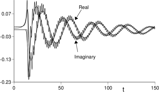
Figure 5.  : Theoretical and numerical results from Ref. [17] for the correlator $\left\langle\sigma^{z}(x,t)\sigma^{z}(0,0)\right\rangle$ of $H_{I}$ at $x=30$ with $J=1$, $g=1.1$ (therefore $\Delta=-0.2$), $T=0.1$ and so the system is in the quantum-disordered region of Fig 3. The numerical data was obtained for a lattice size $L=512$ with free boundary conditions; it has a “ringing” at high frequency due to the lattice cutoff. The theoretical prediction is from the continuum theory prediction in Eq. (54) and is represented by the smoother curve. The envelope of the numerical curve fits the theoretical prediction well.

The theoretical curve was determined from the continuum expression for $K(x,t)$, but the full lattice form for $\varepsilon_{k}$ was used. The theory agrees well with the numerics; some differences are visible for small $x$, outside the light cone, but this is outside the domain of validity of (54).

High $T$, $T\gg|\Delta|$

Right at the critical point, $\Delta=0$, this regime extends all the way down to $T=0$. We begin by writing the $T=0$ equal-time correlator of the continuum theory; from the scaling dimension of $\sigma^{z}$ in (31), this must have the form

$$\left\langle\sigma^{z}(x,0)\sigma^{z}(0,0)\right\rangle\sim\frac{1}{(|x|/c)^{1/4}}~{}~{}~{}~{}~{}~{}\mbox{at $T=0$, $\Delta=0$},$$ (56)

We will now fix the prefactor in (56) using our earlier results. The key ingredient is our knowledge that the underlying continuum model ${\cal L}_{I}$ is is relativistically and conformally invariant at the $T=0$ critical point. Further we assume that the mapping (29) between correlators at $T\neq 0$ from those at $T=0$ holds also for the two point correlator of $\sigma^{z}$ Then from (56) we must have at $T\neq 0$, but $\Delta=0$

$$\left\langle\sigma^{z}(x,i\tau)\sigma^{z}(0,0)\right\rangle\sim T^{1/4}\frac{1}{\left[\sin(\pi T(\tau-ix/c))\sin(\pi T(\tau+ix/c))\right]^{1/8}}.$$ (57)

Notice that we are now working in imaginary time, as it is slightly more convenient for our purposes; the real time result can in this case be obtain by analytic continuation, as we have the exact functional form for $0\leq\tau\leq 1/T$. Let us now use this result in the equal-time case in the regime $xT/c\gg 1$. Precise results for this regime where quoted earlier in (30), where using the values $F_{I}(0)=\pi/4$ (from evaluation of (33)) and $G_{I}(0)=0.858714569\ldots$ we have

$$\left\langle\sigma^{z}(|x|\rightarrow\infty,\tau=0)\sigma^{z}(0,0)\right\rangle=ZT^{1/4}G_{I}(0)\exp\left(-\frac{\pi T|x|}{4c}\right)~{}~{}\mbox{at $\Delta=0$}$$ (58)

Finally, comparing with (57) we obtain, for $\Delta=0$

$$\left\langle\sigma^{z}(x,i\tau)\sigma^{z}(0,0)\right\rangle=ZT^{1/4}\frac{2^{-1/8}G_{I}(0)}{\left[\sin(\pi T(\tau-ix/c))\sin(\pi T(\tau+ix/c))\right]^{1/8}}.$$ (59)

As expected, this result is of the scaling form (35), and indeed completely determines the function $\Phi_{I}$ for the case where its last argument is zero.

Now let us turn to a physical interpretation of the main result (59). Consider first the case $T=0$. By a Fourier transformation of the $T=0$ limit of (59) we obtain the dynamic susceptibility

$$\chi(k,\omega)=Z(4\pi)^{3/4}G_{I}(0)\frac{\Gamma(7/8)}{\Gamma(1/8)}\frac{c}{(c^{2}k^{2}-(\omega+i\delta)^{2})^{7/8}}~{}~{},~{}~{}\mbox{$T=0$, $\Delta=0$}$$ (60)

with $\delta$ a positive infinitesimal. We plot $\mbox{Im}\chi(k,\omega)/\omega$ in Fig 6.

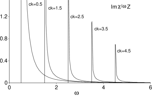
Figure 6.  : Spectral density, $\mbox{Im}\chi(k,\omega)/\omega Z$, of $H_{I}$ at its critical point $g=1$ ($\Delta=0$) at $T=0$, as a function of frequency $\omega$, for a set of values of $k$.

Notice that there are no delta functions in the spectral density like there were in the quantum disordered phase (Fig 2), indicating the absence of any well-defined quasiparticles. Instead, we have a critical continuum of excitations. However, the presence of sharp thresholds and singularities indicates that there is still perfect phase coherence, as there must be in the ground state.

Now let us turn to non-zero $T$. We Fourier transform (59) to obtain $\chi(k,i\omega_{n})$ at the Matsubara frequencies $\omega_{n}$ and then analytically continue to real frequencies (there are some interesting subtleties in the Fourier transform to $\chi(k,i\omega_{n})$ and its analytic structure in the complex $\omega$ plane, which are discussed elsewhere[27]). This gives us the leading result for $\chi(k,\omega)$ in the high $T$ region

$$\chi(k,\omega)=\frac{Zc}{T^{7/4}}\frac{G_{I}(0)}{4\pi}\frac{\Gamma(7/8)}{\Gamma(1/8)}\frac{\displaystyle\Gamma\left(\frac{1}{16}+i\frac{\omega+ck}{4\pi T}\right)\Gamma\left(\frac{1}{16}+i\frac{\omega-ck}{4\pi T}\right)}{\displaystyle\Gamma\left(\frac{15}{16}+i\frac{\omega+ck}{4\pi T}\right)\Gamma\left(\frac{15}{16}+i\frac{\omega-ck}{4\pi T}\right)}.$$ (61)

We show a plot of $\mbox{Im}\chi/\omega$ in Fig 7.

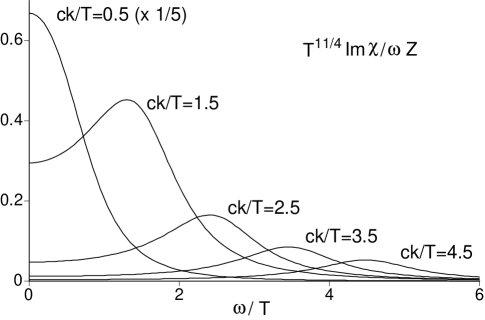
Figure 7.  : The same observable as in Fig 6, $T^{11/4}\mbox{Im}\chi(k,\omega)/\omega Z$, but for $T\neq 0$. This is the leading result for $\mbox{Im}\chi$ for $T\gg|\Delta|$ i.e. in the high $T$ region of Fig 3. All quantities are scaled appropriately with powers of $T$, and the absolute numerical values of both axes are meaningful.

This result is the finite $T$ version of Fig 6. Notice that the sharp features of Fig 6 have been smoothed out on the scale $T$, and there is non-zero absorption at all frequencies. For $\omega,k\gg T$ there is a well-defined peak in $\mbox{Im}\chi/\omega$ (Fig 7) rather like the $T=0$ critical behavior of Fig 6. However, for $\omega,k\ll T$ we cross-over to the quantum relaxational regime [7] and the spectral density $\mbox{Im}\chi/\omega$ is similar to (but not identical) a Lorentzian around $\omega=0$. This relaxational behavior can be characterized by a relaxation rate $\Gamma_{R}$ defined as

$$\Gamma_{R}^{-1}=-i\left.\frac{\partial\ln\chi(0,\omega)}{\partial\omega}\right|_{\omega=0}$$ (62)

(this is motivated by the phenomenological relaxational form $\chi(0,\omega)=\chi_{0}/(1-i\omega/\Gamma_{R}+{\cal O}(\omega^{2}))$). The frequency scale on which the sharp features of Fig 6 have been smoothed out is also $\Gamma_{R}$, and so we may now identify the phase coherence time $\tau_{\varphi}=1/\Gamma_{R}$. From (61) we determine:

$$\frac{1}{\tau_{\varphi}}=\Gamma_{R}=\left(2\tan\frac{\pi}{16}\right)\frac{k_{B}T}{\hbar},$$ (63)

where we have returned to physical units. At the scale of the characteristic rate $\Gamma_{R}$, the dynamics of the system involves intrinsic quantum effects (responsible for the non-Lorentzian lineshape) which cannot be neglected; description by an effective classical model (as was appropriate in both the renormalized classical and quantum disordered regions of Fig 3) would require that $\Gamma_{R}\ll k_{B}T/\hbar$, which is thus not satisfied in the high $T$ region of Fig 3. Alternatively stated, the mean spacing between the thermally excited particles is now of order their de-Broglie wavelength, and so the classical thermal and quantum fluctuations must be treated at an equal footing.

The ease with which our expressions for $\tau_{\varphi}$ in (45,55,63) have been obtained bely their remarkable nature. Notice that we are working in a closed Hamiltonian system, evolving unitarily in time with the operator $e^{-iH_{I}t/\hbar}$, from an initial density matrix given by the Gibbs ensemble at a temperature $T$. Yet, we have obtained relaxational behavior at low frequencies, and determined exact values for a dissipation constant. In contrast, in the theory of dynamics near classical critical points [28], the relaxation dynamics is simply postulated in a rather ad hoc manner, and the relaxational constants are treated as phenomenological parameters to be determined by comparison with experiments.

Summary

The main features of the finite temperature physics of the quantum Ising model are summarized in Figs 3 and Fig 8.

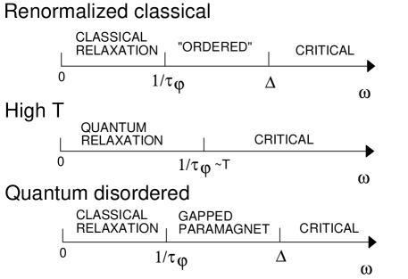
Figure 8.  : Crossovers as a function of frequency for the Ising model in the different regimes of Fig 3. The correlations in the two classical relaxational regimes are quite different from each other. The “ordered” regime is in quotes, because there is no long-range order, and the system only appears ordered between spatial scales $c/\Delta$ and $\xi_{c}$. In the renormalized-classical and quantum-disordered regions $1/\tau_{\varphi}\sim Te^{|\Delta|/T}$.

At short enough times or distances in all three regions of Fig 3, the systems displays critical fluctuations characterized by the dynamic susceptibility (60). The regions are distinguished by their behaviors at the low frequencies and momenta. In both the low $T$ regimes of Fig 3 (renormalized classical and quantum disordered), the long time dynamics is relaxational and is described by effective classical models. The relaxation time, or equivalently, the phase coherence time, is of order $(\hbar/k_{B}T)e^{(\mbox{energy gap})/k_{B}T}$, and is therefore much longer than $\hbar/k_{B}T$. In contrast, the dynamics in the high $T$ region is also relaxational, but involves quantum effects in an essential way, as was described above. In this region the phase relaxation time is now of order $\hbar/k_{B}T$.

Finally a few remarks about experiments. While there are no experimental studies of the Ising chain in a transverse field, the quantum relaxational dynamics of its critical point $g=1$ is very closely related to the finite temperature dynamics of $S=1/2$ Heisenberg spin chains. The spin correlators of the latter system are given by expressions very similar to those in Section 2.3, and the relaxational dynamics can has been experimentally probed in NMR experiments. There is good agreement between theory and experiments, and the reader is referred to some recent papers for further details [29, 30, 31].

3 $O(3)$ quantum rotors between one and three dimensions

This section will examine ${\cal S}$ for $N=3$ in $d=1,2,3$: the $N=3$ model describes the low energy physics of quantum antiferromagnets, and we will present a number of experimental applications.

Many aspects of the physics will be similar to those described in Section 2 for the $N=1$, $d=1$ case. However there are some genuinely new features which shall be the focus of our attention. For $N\geq 2$, ${\cal S}$ has a continuous $O(N)$ symmetry, and associated conserved charges, whose transport properties will be of interest to us. Further, for $d>2$, there is a thermodynamic phase transition at a non-zero temperature: we shall briefly consider the subtle interplay between the critical singularities of the non-zero temperature transition and those of the $T=0$ quantum critical point.

As in the Ising case, it is useful to take a Hamiltonian point of view. In this case (see Section 3.2 for justification) the associated model is the following Hamiltonian of $O(N)$ quantum rotors on the sites $i$ of a regular $d$ dimensional lattice (we will consider general $N\geq 2$ for completeness):

$$H_{R}=\frac{Jg}{2}\sum_{i}\stackrel{{\scriptstyle\leftrightarrow}}{{L^{2}}}_{i}-J\sum_{\langle ij\rangle}\vec{n}_{i}\cdot\vec{n}_{j},$$ (64)

where the sum $\langle ij\rangle$ is over nearest neighbors, $J>0$ is an overall energy scale, and $g>0$ is a dimensionless coupling constant. The $N$ component vectors $\vec{n}_{i}$ are of unit length, $\vec{n}_{i}^{2}=1$, and represent the orientation of the rotors on the surface of a sphere in $N$-dimensional rotor space; as we will see later, $\vec{n}\rightarrow\phi_{\alpha}$ in the mapping to the CQFT ${\cal S}$. The operators ${L}_{i\mu\nu}$ ($\mu<\nu$, $\mu$, $\nu=1\ldots N$) are the $N(N-1)/2$ components of the angular momentum $\stackrel{{\scriptstyle\leftrightarrow}}{{L}}_{i}$ of the rotor: the first term in $H_{R}$ is the kinetic energy of the rotor with $1/g$ the moment of inertia. The different components of $\vec{n}_{i}$ constitute a complete set of commuting observables and the state of the system can be described by a wavefunction $\Psi(\vec{n}_{i})$. The action of $\stackrel{{\scriptstyle\leftrightarrow}}{{L}}_{i}$ on $\Psi$ is given by the usual differential form of the angular momentum

$$L_{i\mu\nu}=-i\left(n_{i\mu}\frac{\partial}{\partial n_{i\nu}}-n_{i\nu}\frac{\partial}{\partial n_{i\mu}}\right).$$ (65)

The commutation relations among the $\stackrel{{\scriptstyle\leftrightarrow}}{{L}}_{i}$ and $\vec{n}_{i}$ can now be easily deduced. We emphasize the difference of the rotors from Heisenberg-Dirac quantum spins: the components of the latter at the same site do not commute, whereas the components of the $\vec{n}_{i}$ do.

While there are no direct realizations of quantum rotors in nature, they are a useful model of the low energy physics of a number of experimental systems. As we will see below, a quantum rotor should be considered as a model for the physics of a pair of antiferromagnetically coupled Heisenberg spins. The field $\vec{n}$ represents to the staggered antiferromagnetic order parameter, while $\stackrel{{\scriptstyle\leftrightarrow}}{{L}}$ is the total magnetization. Thus quantum rotor models describe the spin fluctuations of the spin-ladder compounds [32], a rotor representing the spins on each rung of the ladder. For technical reasons not explored here, the rotor models also describe integer spin chains, and a large class of Heisenberg antiferromagnets in higher dimensions. Finally, rotor models are also useful in double-layer quantum Hall systems [33], where superexchange effects lead to an antiferromagnetic coupling between the electrons in the two layers [34]. These systems (excluding the double-layer quantum Hall system for which the reader is referred to the literature) will be described in more detail in the following subsections.

There is a strong analogy between the rotor Hamiltonian $H_{R}$ in (64) and the Ising Hamiltonian $H_{I}$ in (5). We will be looking at the transition between a magnetically ordered state with $\langle\vec{n}\rangle\neq 0$ and $O(N)$ symmetry broken, and a quantum paramagnet in which correlations of $\vec{n}$ are short ranged. As in the Ising model, it is the exchage term, proportional to $J$, that favors the ordered state, while the ‘kinetic energy’, proportional to $Jg$ leads to fluctuations in the orientation of the order parameter and eventually to loss of long-range order. The similarity between the two models will also be apparent in the strong (large $g$) and weak coupling (small $g$) analyses in the following section.

3.1 Limiting cases

The pictures which emerge in the following two perturbative analyses are expected to hold on either side of a quantum critical point at $g=g_{c}$.

Strong coupling $g\gg 1$

At $g=\infty$, the exchange term in $H_{R}$ can be neglected, and the Hamiltonian decouples into independent sites, and can be diagonalized exactly. The eigenstates on each site are the eigenstates of $\stackrel{{\scriptstyle\leftrightarrow}}{{L^{2}}}$; for $N=3$ these are the states

$$\left|\ell,m\right\rangle_{i}~{}~{}~{}\ell=0,1,2,\ldots,~{}-\ell\leq m\leq\ell$$ (66)

and have eigenenergy $Jg\ell(\ell+1)/2$. Compare this single site spectrum with that of a pair of Heisenberg-Dirac spin $S$ quantum spins with an antiferromagnetic exchange $K$; for a suitably chosen $K$ we get the same sequence of levels and energies but with a maximum allowed value of $\ell=2S$. Assuming this upper cutoff is not crucial for the low energy physics, we can use a single quantum rotor is an effective model for a pair of spins.

The ground state of $H_{R}$ in the large $g$ limit consists of the quantum paramagnetic state with $\ell=0$ on every site:

$$|0\rangle=\prod_{i}|\ell=0,m=0\rangle_{i}$$ (67)

Compare this with strong coupling ground state (7) of the Ising model. Indeed, the remainder of the strong coupling analysis of Section 2.1 can borrowed here for the rotor model, and we can therefore be quite brief. The lowest excited state is a ‘particle’ in which a single site has $\ell=1$, and this excitation hops from site to site. An important difference from the Ising model is that this particle is three-fold degenerate, corresponding to the three allowed values $m$. The dynamic susceptibility has a quasiparticle pole at the energy of this particle, and odd particle continua above the three particle threshold.

Weak coupling, $g\ll 1$

At $g=0$, the ground state breaks $O(N)$ symmetry, and all the $\vec{n}_{i}$ vectors orient themselves in a common, but arbitrary direction. Excitations above this state consist of ‘spin waves’ which can have an arbitrarily low energy. This is a crucial difference from the Ising model, in which there was an energy gap above the ground state. The presence of gapless spin excitations is a direct consequence of the continuous $O(N)$ symmetry of $H_{R}$: we can make very slow deformations in the orientation of $\langle\vec{n}\rangle$, and get an orthogonal state whose energy is arbitrarily close to that of the ground state. Explicitly, for $N=3$, and a ground state polarized along $(1,0,0)$ we parametrize

$$\vec{n}(x,t)=(1,\pi_{1}(x,t),\pi_{2}(x,t))$$ (68)

where $|\pi_{1}|,|\pi_{2}|\ll 1$, and look at the linearized equations of motion for $\pi_{1}$, $\pi_{2}$. A standard calculation then gives harmonic spin waves with energy $\omega=ck$ ($c$ is the spin wave velocity); their wavefunctions can then be constructed using harmonic oscillator states.

3.2 Continuum theory and large $N$ limit

To obtain the path integral representation of the quantum mechanics of $H_{R}$, we interpret the $\vec{n}_{i}$ as the co-ordinates of particles constrained to move on the surface of a sphere in $N$ dimensions: we can then simple use the standard Feynman path integral representation of single-particle quantum mechanics. After taking the continuum limit, such a procedure gives

$$Z=\int{\cal D}\vec{n}(x,\tau)\delta(\vec{n}^{2}(x,\tau)-1)\exp\left(-\int_{0}^{1/T}d\tau\int d^{d}x{\cal L}\right)$$

$${\cal L}=\frac{N}{2c\tilde{g}}\left[c^{2}\left(\frac{\partial\vec{n}}{\partial x_{i}}\right)^{2}+\left(\frac{\partial\vec{n}}{\partial\tau}\right)^{2}\right]$$ (69)

Here $c\sim Ja$ is a velocity which will turn out to be the spin wave velocity, and we have set $\hbar=k_{B}=1$. The prefactor of $N$ is for future convenience. The coupling constant $\tilde{g}\sim ga^{d-1}$ has the dimensions of $(\mbox{length})^{d-1}$; we will not use the original $g$ in $H_{R}$ further in this discussion, and we will drop the tilde in $\tilde{g}$ from now. The above action is valid only at long distances and times, so there is an implicit cutoff above momenta of order $\Lambda\sim 1/a$ and frequencies of order $c\Lambda$. Our main interest here shall be the universal physics at scales much smaller than $\Lambda$. It is now also apparent that if we convert the fixed length field $\vec{n}$ to the “soft” spin $\phi_{\alpha}$, the action in (69) maps to the model ${\cal S}$.

A useful tool in the analysis of (69) is the limit of a large number of components of $\vec{n}$ i.e. expansion in $1/N$ [7]. For $N\geq 3$, the $N=\infty$ solution already contains the proper dilineation of all the crossovers and phase transitions for all $d$. The description of the dynamic properties however requires a fairly subtle analysis of the fluctuations. As all of these issues have been discussed at length in the literature, here we will merely set-up the framework of the $N=\infty$ theory, and then proceed to a physical discussion of the properties of the various regimes for $d=1,2,3$.

The $N=\infty$ solution is quite easy to set up, at least in the phase without long range order in the order parameter $\vec{n}$; we will not discuss the ordered phase [7] here. We rescale the $\vec{n}$ field to

$$\vec{\tilde{n}}=\sqrt{N}\vec{n},$$ (70)

and impose the $\vec{\tilde{n}}^{2}=N$ constraint by a Lagrange multiplier, $\lambda$. The action is then quadratic in the $\vec{\tilde{n}}$ field, which can then be integrated out to yield

$$Z=\int{\cal D}\lambda\exp\left[-\frac{N}{2}\left(\mbox{Tr}\ln(-c^{2}\partial_{i}^{2}-\partial_{\tau}^{2}+i\lambda)-\frac{i}{cg}\int_{0}^{1/T}d\tau\int d^{d}x\lambda\right)\right]$$ (71)

The action now has a prefactor of $N$, and the $N=\infty$ limit of the functional integral is therefore given exactly by its saddle point value. We assume that the saddle-point value of $\lambda$ is space and time independent, and given by $i\lambda=\sigma^{2}$. The saddle-point equation determining the value of the parameter $\sigma^{2}$ is

$$\int^{\Lambda}\frac{d^{d}k}{(2\pi)^{d}}T\sum_{\omega_{n}}\frac{1}{c^{2}k^{2}+\omega_{n}^{2}+\sigma^{2}}=\frac{1}{cg},$$ (72)

where the sum over $\omega_{n}$ extends over the Matsubara frequencies $\omega_{n}=2n\pi T$, $n$ integer. It is also not difficult to see that the retarded dynamic susceptibility $\chi(k,\omega)$, which is the two-point correlator of the $n$ field, is given by

$$\chi(k,\omega)=\frac{cg/N}{c^{2}k^{2}-(\omega+i\delta)^{2}+\sigma^{2}},$$ (73)

at $N=\infty$, with $\delta$ a positive infinitesimal. The Eqns (72,73) are the central results of the $N=\infty$ theory; in spite of their extremely simple structure, these equations contain a great deal of information, and it takes a rather subtle and careful analysis to extract the universal information contained in them [7]. We will not go into these technical details here, but will be satisfied by describing the different physical regimes predicted by (72,73) and other analyses of $H_{R}$.

3.3 Dynamics in one dimension: application to spin-gap compounds

Solution of (72) in $d=1$ shows that there is an energy gap, $\Delta$, for all positive values of $g$. Even for very small values of $g$, where one might expect long-range order, and the weak coupling solution of (3.1) to apply, quantum fluctuations are strong enough to always drive the system paramagnetic. For small $g$, the energy gap behaves like

$$\Delta\sim c\Lambda e^{-2\pi/g}.$$ (74)

This behavior can be confirmed by a more sophisticated renormalization group analysis [35]. The implication of this important result is that the large $g$ analysis of Section 3.1 actually applies for all values of $g$ in $d=1$.

The finite $T$ crossovers can also be deduced by a solution of (72) [36], and are sketched in Fig 9.

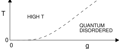
Figure 9.  : Crossovers of $H_{R}$ (Eq. (64)) in $d=1$ for $N\geq 3$. The phase boundary is at $\Delta\sim T$, with $\Delta$ given by (74).

The quantum critical point of Fig 3 has effectively been moved to $g=0$, and there are now only $T$ distinct limiting physical regimes: (i) $T\ll\Delta$, where strong quantum fluctuations create a singlet paramagnetic ground state, and we have a few thermally excited elementary excitations—for $N=3$ these are a triplet of spin 1 particles with energy $(\Delta^{2}+c^{2}k^{2})^{1/2}$ at momentum $k$, and correspond (crudely) to breaking a singlet valence bond between two neighboring spins in the underlying antiferromagnet; (ii) $\Delta\ll T\ll c\Lambda$, the high $T$ regime of the continuum theory, where quantum fluctuations are marginally subdominant to thermal fluctuations [37] (by a factor of $1/\ln(T/\Delta)$), and we can locally describe the system in terms of a doublet of left/right circularly polarized spin-waves about an ordered state—however, interactions of thermally excited spin waves lead again to a paramagnetic state.

Below we will present an exact theory for dynamic and transport properties in the $T\ll\Delta$ regime [38]. There is as yet no complete theory for dynamics in the $T\gg\Delta$ regime, and its description remains an important open problem.

The basic approach followed for $T\ll\Delta$ is very similar to that taken for the quantum-disordered region of the Ising chain in Section 2.3. The central difference here is that the quasi-particle excitations have an additional spin label, $m=1\ldots N$. We will present our discussion below for the physical case $N=3$, although the generalization to arbitrary $N$ is immediate. This label on the quasiparticles is associated with the conserved $O(N)$ charge, which is the total spin $\sum_{i}\vec{L}_{i}$. We shall restrict our attention here to the dynamics associated with the transport of this conserved charge: this will be described by obtaining the exact long-time form of the correlator

$$C_{\alpha\beta}(x,t)=\left\langle L_{\alpha}(x,t)L_{\beta}(0,0)\right\rangle$$ (75)

For the case $N=3$, the second-rank antisymmetric tensor indices $\mu\nu$ on $L$ have been replaced by a single vector index $\alpha$ or $\beta$. The method described below can also be used to obtain dynamic correlators of the $\vec{n}$ field: this will be discussed elsewhere [39].

There are two key observations that allow our exact computation for $T\ll\Delta$. The first, as in the Ising chain, is that as the density of particles $\sim e^{-\Delta/T}$, and their mean spacing is much larger than their thermal de-Broglie wavelength $\sim c/(\Delta T)^{-1/2}$; as a result the particles can be treated semiclassically. The density of particles with each spin $m$ ($m=-1,0,1$ for $N=3$) is now given by the expression (39), and the total density therefore equals $3\rho$. The second observation is that collisions between these particles are described by their known two-particle $S$-matrix [40], and only a simple limit of this $S$-matrix is needed in the low $T$ limit. The r.m.s. velocity of a thermally excited particle $v_{T}=c(T/\Delta)^{1/2}$, and hence its ‘rapidity’ $\sim v_{T}/c\ll 1$. In this limit, the $S$-matrix for the process in Fig 10 is [40]

$${S}^{m_{1}m_{2}}_{m^{\prime}_{1},m^{\prime}_{2}}=(-1)\delta_{m_{1}m^{\prime}_{2}}\delta_{m_{2}m^{\prime}_{1}}.$$ (76)

In other words, the excitations behave like impenetrable particles which preserve their spin in a collision. As in the Ising chain, energy and momentum conservation in $d=1$ require that these particles simply exchange momenta across a collision (Fig 10).

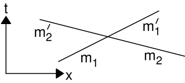
Figure 10.  : Two particle collision described by the $S$-matrix (76). The momenta before and after the collision are the same, so the figure also represents the spacetime trajectories of the particles.

The $(-1)$ factor in (76) can be interpreted as the phase-shift of repulsive scattering between slowly moving bosons in $d=1$. Indeed, the simple form of (76) is due to the slow motion of the particles, and is not a special feature of relativistic continuum theory: it can be shown that (76) also holds for lattice Heisenberg spin chains in the limit of vanishing velocities.

As in Sections 2.3 and 2.3, we represent $C(x,t)$ as a ‘double time’ path integral, and in the classical limit, stationary phase is achieved when the trajectories are time-reversed pairs of classical paths (Fig 11).

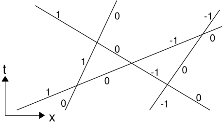
Figure 11.  : A typical set of particle trajectories contributing to $C(x,t)$. Each trajectory represents paths moving both forward and backward in time, and the $(-1)$ phase at each collision is neutralized by its time-reversed contribution. The particle co-ordinates are $x_{k}(t)$, with the labels $k$ chosen so that $x_{k}(t)\leq x_{l}(t)$ for all $t$ and $k<\ell$. Shown on the trajectories are the values of the particle spins $m_{k}$ which are independent of $t$ in the low $T$ limit.

Each trajectory has a spin label, $m$, which obeys (76) at each collision. The label, $m$, is assigned randomly at some initial time with equal probability, but then evolves in time as discussed above (Fig 11). We label the particles consecutively from left to right by an integer $k$; then their spins $m_{k}$ are independent of $t$, and we denote their trajectories $x_{k}(t)$. The longitudinal correlation $C_{33}$ is then given by the correlators of the classical observable

$$L_{3}(x,t)=\sum_{k}m_{k}\delta(x-x_{k}(t))$$ (77)

in the classical ensemble defined in Section 2.3 and above. Now because the spin and spatial co-ordinates are independently distributed, the correlators of $m_{k}$ and $x_{k}$ factorize. The $m_{k}$ are uncorrelated, and therefore $\langle m_{k}m_{\ell}\rangle=(2/3)\delta_{k\ell}$ We therefore have

$$C_{33}(x-x^{\prime},t-t^{\prime})=\frac{2}{3}\sum_{k}\left\langle\delta(x-x_{k}(t))\delta(x^{\prime}-x_{k}(t^{\prime}))\right\rangle$$ (78)

This result involves the self two-point correlation of a given particle $k$, which follows a complicated trajectory in the way we have labeled the particles (e.g. the trajectory of the $-1$ in Fig 11). Fortunately, precisely this correlator was considered three decades ago by Jepsen [41] and a little later by others [42]; they showed that, at sufficiently long times, this correlator has a Brownian motion form. Inserting their results into (78), we obtain the results presented below.

An important property of the results is that they can written in a ‘reduced’ scaling form [7], much like that found in Sections 2.3 and 2.3. The characteristic spatial length ($L_{x}$) and time ($L_{t}$) can be chosen to be

$$L_{x}=\frac{1}{3\rho}~{}~{}~{}~{}~{}L_{t}=\frac{1}{3\rho}\left(\frac{\Delta}{2c^{2}T}\right)^{1/2}.$$ (79)

Notice $L_{x}\sim ce^{\Delta/T}/\sqrt{\Delta T}$ is the mean spacing between the particles , and $L_{t}\sim e^{\Delta/T}/T$ is a typical time between particle collisions. Our final result is

$$C_{\alpha\beta}(x,t)=6\rho^{2}F\left(\frac{|x|}{L_{x}},\frac{|t|}{L_{t}}\right)\delta_{\alpha\beta}$$ (80)

where $F$ is a universal scaling function. A complete expression for $F$ is given in Ref [38]. Here we note the important limiting forms. For short times $F$ has the ballistic form

$$F(\bar{x},\bar{t})\approx e^{-\bar{x}^{2}/\bar{t}^{2}}/\bar{t}\sqrt{\pi},$$ (81)

which is the auto-correlator of a classical ideal gas in $d=1$, and holds for $|\bar{t}|\ll|\bar{x}|\ll 1$. In contrast, for $|\bar{t}|\gg 1,|\bar{x}|$ it crosses over to the diffusive form

$$F(\bar{x},\bar{t})\approx\frac{e^{-\sqrt{\pi}\bar{x}^{2}/2\bar{t}}}{(4\pi\bar{t}^{2})^{1/4}}$$ (82)

In the original dimensionful units, (79) and (82) imply a spin diffusion constant, $D_{s}$, given exactly by

$$D_{s}=\frac{c^{2}e^{\Delta/T}}{3\Delta}.$$ (83)

To the best of our knowledge, this is first exact result for the spin diffusivity in any paramagnetic spin system.

The above long-time diffusive form of the magnetization correlations have important consequences for NMR experiments on one-dimensional compounds with a spin gap. The comparison with experiments requires generalization of the above theory to include an external magnetic field $H$. This has been discussed elsewhere [38]. From this computation one finds that the longitudinal nuclear spin relaxation rate, $1/T_{1}$, is given in the weak field limit $H\ll\Delta,L_{t}^{-1}$ by

$$\frac{1}{T_{1}}=\frac{\Gamma T\chi}{\sqrt{2D_{s}H}}=\frac{\Gamma\Delta e^{-3\Delta/2T}}{c^{2}}\sqrt{\frac{3T}{\pi H}}~{}~{};~{}~{}\chi_{u}=\frac{e^{-\Delta/T}}{c}\sqrt{\frac{2\Delta}{\pi T}},$$

where $\Gamma$ is a nuclear hyperfine coupling, and $\chi_{u}$ is the paramagnetic spin susceptibility (in the rotor model, this is the linear response to a field $H$ under which $H_{R}\rightarrow H_{R}-H\sum_{i}L_{i3}$). For experimental comparisons, a striking property of the above, pointed out to us by M. Takigawa, is that the low $T$ activation gaps for $1/T_{1}$ ($\Delta_{1/T_{1}}$) and $\chi$ ($\Delta_{\chi}$) satisfy $\Delta_{1/T_{1}}/\Delta_{\chi}=3/2$.

Values for the activation gaps $\Delta_{1/T_{1}}$ and $\Delta_{\chi}$ have been quoted for a number of experimental systems [43, 44, 32], and it has consistently been found that $\Delta_{1/T_{1}}$ is larger than $\Delta_{\chi}$. The above theoretical results provide a natural explanation for this puzzling experimental trend. This is further explored in Fig 12, which was kindly provided to us by H. Yasuoka.

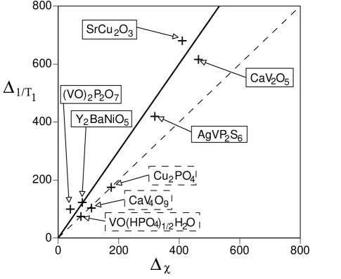
Figure 12.  : Measured values of the activation gaps $\Delta_{1/T_{1}}$ and $\Delta_{\chi}$ for a number of spin gap systems. The one-dimensional compounds are enclosed by full rectangles, while others have dashed rectangles (these are either two-dimensional or consist of isolated dimers). The full line is the theoretically predicted ratio of $3/2$ and is in good agreement with the trends in the $d=1$ systems. The other systems have a ratio close to unity, and this is expected to be the case when elastic impurity-scattering of the quasiparticles dominates.

We have also compared [39] the detailed $H$ and $T$ dependence of the $1/T_{1}$ measurements on Ref [43] with the predictions of our theory. These measurements have enough dynamic range to explore the ballistic-diffusive crossover described above, and the results are in good agreement with theoretical predictions.

3.4 Two dimensions

Solution of the $N=\infty$ equation (72) in $d=2$ yields a phase diagram essentially identical to that shown in Fig 3 for the $d=1$ quantum Ising model. A renormalization group analysis [21] shows that these large $N$ results are qualitatively correct for the physical case of $N=3$. A detailed description of the physical properties in the different regions of the phase diagram of Fig 3 for the $d=2$ $O(3)$ rotor model has been obtained in the $1/N$ expansion [7]. We will not describe this analysis here as the physical properties are quite similar to those for the $d=1$ Ising model, which we have discussed in some detail in Section 2. Further, the results of the large $N$ theory have been reviewed elsewhere [3, 45].

We do note one important difference from the $d=1$ Ising model, however. The ordered phase ($g<g_{c}$) of the $d=2$ $O(3)$ rotor model has gapless spin-wave excitations above the ground state, unlike the Ising model which had a gap. Consequently, we need a different energy scale to characterize the deviation of the ground state from the quantum critical point $g=g_{c}$. A convenient choice is the spin stiffness, $\rho_{s}$, which has the dimensions of energy in $d=2$. The non-zero $T$ properties of the rotor model will now be universal functions of the dimensionless ratio $\rho_{s}/T$ for $g<g_{c}$. The renormalized-classical region is therefore present for $T<\rho_{s}$, while the “High T” region is $T>\rho_{s}$. There is an energy gap, $\Delta$, towards a triplet of quasiparticle excitations in the quantum-disordered phase present for $g>g_{c}$, and the nonzero $T$ crossovers in this case are very similar to those of the $d=1$ Ising model: the physics is “quantum-disordered” for $T<\Delta$, and “High T” for $T>\Delta$.

The $d=2$ $O(3)$ rotor model is expected to describe the low energy properties two dimensional quantum antiferromagnets whose low energy states are well described by fluctuations of a collinear antiferromagnetic spin ordering. The $S=1/2$ spin-1/2 square lattice antiferromagnet, realized in ${\rm La}_{2}{\rm CuO}_{4}$ and related insulators, is an important example of such a system, and we now discuss the relationship of its properties to those of the rotor model. By a comparison with low temperature behavior of the correlation length observed in neutron scattering measurements, Chakravarty et al. [21] convincingly argued that the ground state of this model has long-range Néel order, i.e. it maps onto the rotor model with a coupling $g<g_{c}$. Their analysis was restricted to the renormalized classical region of Fig 3 i.e. $T\ll\rho_{s}$, where static properties reduce to those of an effective classical rotor model. A theory for the dynamic properties in this region was presented in Ref [46] by postulating classical equations of motion for the classical rotor model.

Next, we turn to a question [47] which arises naturally from the structure of Fig 3: does the $S=1/2$ square lattice antiferromagnet crossover into the “High T” regime at temperatures $T>\rho_{s}$ ? The existence of such a crossover is subject to the condition that it occur at temperatures small enough so that the mapping to rotor model remains valid. Strong evidence for the “High T” regime was found in Ref [47] by a comparison of the $1/N$ expansion of the rotor model with numerical and experimental measurements of the uniform susceptibitlity. The magnitude and temperature dependence of the $1/T_{1}$ [48] and $1/T_{2G}$ [49] nuclear magnetic relaxation rate measurements on ${\rm La}_{2}{\rm CuO}_{4}$ were also found to be in good agreement with theory [7, 50]. Convincing evidence for the renormalized-classical to “High T” crossover was presented by Sokol et al. [51] and Elstner et al. [52] using a high temperature series expansion for a number of static correlators of the $S=1/2$ square lattice antiferromagnet. (Elstner et al. [52] also examined the $S=1$ square lattice antiferromagnet, and found no evidence for the “High T” regime; this indicates, as expected, that the effective value of $g$ for $S=1$ is significantly smaller than $g_{c}$.) It was also argued early on [47] that the $T$ dependence of the correlation length, which was central to the conclusions of Chakravarty et al. , would not exhibit a clear signature of the “High T” regime. This point was subsequently reiterated by Greven et al. [53].

A more complete understanding of the physics of the “High T” regime should emerge from a careful study of the wavevector, frequency, and temperature dependence of the imaginary part of the staggered dynamic spin susceptiblity. This should obey a scaling form [6] much like that obtained earlier for the Ising model in (61):

$$\chi^{\prime\prime}(k,\omega)=\frac{{\cal A}}{T^{2-\eta}}\Phi_{\chi}\left(\frac{\hbar ck}{k_{B}T},\frac{\hbar\omega}{k_{B}T}\right),$$ (84)

where ${\cal A}$ is a non-universal amplitude and $\eta$ is the anomalous dimension of $\vec{n}$ field at the quantum-critical point ($\eta\approx 0.03$ for $d=2$, $N=3$). Detailed theoretical results for the form of the universal scaling function $\Phi_{\chi}$ have been obtained [6, 7] in the $1/N$ expansion. Unfortunately there are no existing results for $\chi^{\prime\prime}(k,\omega)$ in ${\rm La}_{2}{\rm CuO}_{4}$ at $T>\rho_{s}$, as the neutron scattering intensity becomes quite small at higher temperatures. However there are other two-dimensional square lattice antiferromagnets with a smaller $\rho_{s}$ [54] which are good candidates for such a study.

This is a good point to make some speculative remarks about the doped antiferromagnet ${\rm La}_{2-x}{\rm Sr}_{x}{\rm CuO}_{4}$. The $1/T_{1}$ measurements of Ref [48] have the striking property that while the low $T$ values of $1/T_{1}$ are quite strongly doping dependent, at higher $T$ $1/T_{1}$ approaches a value which is both temperature and doping-concentration independent. This appears to receive a natural explanation within the framework of a rotor model quantum-critical point. Assuming the main effect of doping is merely to shift the value of the effective coupling constant $g$, the properties of the “High T” region of Fig 3 are determined primarily by the value of $T$ alone, and are insensitive to the precise value of $g$: indeed, in this region, the system does not ‘know’ whether $g$ is smaller or larger than $g_{c}$. Further, the $T$ dependence is predicted to be $1/T_{1}\sim T^{\eta}$ [47, 7], and given the small value of $\eta$, this is essentially $T$-independent. Lastly, the coefficient of $T^{\eta}$ has also been estimated [7] and is consistent with the experimental value.

We turn now to other antiferromagnets in $d=2$ which have a collinear Néel ordered ground state. An interesting system in which it is possible to tune the value of the effective coupling $g$ across $g_{c}$ is the double layer square lattice $S=1/2$ antiferromagnet [55]. This model consists of spin-1/2 Heisenberg spins on two adjacent square lattices, with an intralayer antiferromagnetic exchange $J$ and an interlayer antiferromagnetic exchange $K$. The ratio $K/J$ acts much like the dimensionless coupling $g$, with the large $K/J$ phase a gapped quantum paramagnet of singlet pairs of spins in opposite layers, and the small $K/J$ phase Néel ordered. Numerical simulations have been carried out on this model by Sandvik and collaborators [56], and the critical point $g=g_{c}$ identified rather reasonably well. A number of universal amplitude ratios have been studied at this point, and all results are now in good agreement with the $1/N$ expansion on the $O(N)$ quantum rotor model. High temperature [52, 57] and strong coupling [58] series expansions on the double-layer model also reach a similar conclusion.

An exciting recent development has been the remarkably high precision study of quantum-critical properties in the 1/5-depleted square lattice by Troyer et al. [59]. This is another model in which $g$ can be tuned across $g_{c}$ by varying the ratio of exchange constants. This particular lattice has the additional feature that the mapping to the rotor model is expected to be incomplete: there are additional Berry phases generated by the dynamics of the Heisenberg spins undergoing a “hedgehog” tunneling event [60]. It was argued [7] that such perturbations should be “dangerously irrelevant”, and that they do not modify any of the universal scaling predictions of the rotor model. The results of Troyer et al. are in excellent agreement with the critical properties of the rotor model [59], thus supporting the neglect of the Berry phases.

3.5 Three dimensions

Solution of the $N=\infty$ equation (72) now yields the phase digram shown in Fig 13 [45].

Figure 13.  : Phase diagram for the $O(N)$ rotor model with for $N>2$ and $d=3$. A similar diagram applies for the cases with $N=1,2$ and $d=2,3$. The dashed lines are crossovers, while the full line is the locus of finite temperature phase transitions. The shaded region is where the reduced classical scaling functions apply.

The new feature is presence of a finite temperature phase transition: this lies entirely within the low $T$ region for $g<g_{c}$ and is not a direct property of the quantum critical point. The well-studied classical critical behavior appears only within the shaded region of Fig 13. The quantum-critical scaling functions contain this classical criticality as “reduced scaling functions” in much the same way that in the $d=1$ Ising model the classical function (46) was contained in the more general quantum function in (35). This phenomenon can be studied with the $1/N$ expansion [45], and has also recently been described in an expansion in $\epsilon=3-d$ [8]. Also, because $d=3$ is the upper-critical dimension of ${\cal S}$, there are logarithmic violations of scaling near the quantum-critical point.

Normand and Rice [61] have proposed an interesting recent experimental realization of such a three-dimensional quantum critical point in ${\rm LaCuO}_{2.5}$. This is a spin-ladder compound in which the ladders are moderately strongly coupled in three dimensions. By varying the ratio of the intra-ladder to inter-ladder exchange it is possible to drive such an antiferromagnet across a $d=3$ quantum critical point separating Néel ordered and quantum paramagnetic phases. The uniform susceptibility has a $T^{2}$ dependence at intermediate $T$, which is characteristic of the “High T” region in $d=3$. The entire $T$ dependence of the uniform susceptibility has been compared with large $N$ and quantum Monte Carlo simulations of the quantum-critical model [59], with good agreement.

4 Quantum relaxational transport in two dimensions

Transport properties of the model ${\cal S}$ were considered earlier in Section 3.3. There we determined the spin diffusion constant in the quantum-disordered regime ($T\ll\Delta$) of the $N=3$ model in $d=1$. Here, following Ref [63], we shall describe transport for $N\geq 2$ in $d=2$ in the “High T” region (Fig 1 and 3), where the dynamics is quantum-relaxational (Fig 8) . The methods discussed here can also be applied to the quantum-disordered region of the $N\geq 2$, $d=2$ models, but we shall not present that extension here. Let us also recall that there is one region for which there is no quantitative theory of transport phenomena: the “High $T$” region for $N\geq 3$ in $d=1$; this region should be experimentally accessible in $S=2$ spin chains.

We shall present our discussion using the language of the $N=2$ system, although closely related results apply to all $N\geq 2$. The $N=2$ model describes a superfluid-Mott insulator transition in a lattice boson model with short-range repulsive interactions [64]. The complex superfluid order parameter $\Psi$ is related to the field $\phi_{\alpha}$ by

$$\Psi=(\phi_{1}+i\phi_{2})/\sqrt{2}$$ (85)

(and similarly to $\vec{n}$). It therefore serves a starting point for understanding superfluid-insulator transitions in disordered thin films [65, 66] and Josephson junction arrays [67] and the transitions among quantum Hall states [68, 69, 70].

Rather than describing the transport in terms of the diffusivity, it is more convenient here, both theoretically and experimentally, to characterize it using the conductivity, $\sigma$; the two quantities are, of course, connected by the Einstein relation. We consider the response of ${\cal S}$ to a spatially varying “chemical potential”, $\mu$, (this is the field that couples to the conserved charge for $N=2$; for the $N=3$ case we called it the “magnetic field”) under which the rotor model Hamiltonian transforms as

$$H_{R}\rightarrow H_{R}-Q\sum_{i}\mu(i)L_{i}.$$ (86)

Here $Q$ is the charge of the $\Psi$ field. Note that for $N=2$ there is only one generator $L$ which therefore does not carry any vector indices. In an open system, the expectation value of the current (this is the current associated with the conserved charge) will be proportional to the gradient of $\mu$, and the proportionality constant is $\sigma$. We will be interested here in the $\omega$ and $T$ dependence of $\sigma$ at the critical point $g=g_{c}$, as that controls the value of $\sigma$ in the “High T” region. We begin by writing down the expected scaling form this must satisfy. For this we need the scaling and engineering dimensions of $\sigma$. Rather general arguments [71, 72, 73, 68] show that in $d=2$, $\sigma$ has scaling dimension zero, and engineering dimensions of the quantum unit of conductance $Q^{2}/\hbar$. This leads to the scaling form

$$\sigma=\frac{Q^{2}}{\hbar}\Sigma\left(\frac{\hbar\omega}{k_{B}T}\right)$$ (87)

where $\Sigma$ is a universal scaling function whose properties we will describe here.

It is clear from (87) that the experimentally measured d.c. conductivity is determined by the universal number $\Sigma(0)$. In contrast, any computation of the conductivity performed at $T=0$, in which the $\omega\rightarrow 0$ limit is taken subsequently will determine the number $\Sigma(\infty)$. It was argued quite generally by Cha et al. [72] and Wallin et al. [74] that $\Sigma$ is in independent of $\omega/T$, which therefore also implies that $\Sigma(0)=\Sigma(\infty)$. As a result, there were a number of analytic computations [71, 72, 75, 76, 77, 78, 79, 80, 81] and an exact diagonalization study [82] of the value of $\Sigma(\infty)$ in a variety of models which display a quantum-critical point in $d=2$. Quantum Monte Carlo studies [72, 74, 83, 84, 85] determined the conductivity by analytic continuation from imaginary time data at $\omega=2\pi nTi$, with $n\geq 1$ integer; as the smallest value of $\omega$ is $2\pi Ti$, these studies were effectively also in the regime $|\omega|\gg T$.

The picture of quantum relaxational dynamics we have reviewed in this paper makes it quite clear that the underlying assumption of these works is incorrect: $\Sigma$ is in fact, not independent of $\omega/T$. As we have discussed here, the characteristic property of the “High T” region is that there is a phase relaxation time $\tau_{\varphi}\sim\hbar/k_{B}T$. Dynamic order parameter fluctuations also carry charge, and therefore inelastic collisions between thermally excited charge-carrying excitations will lead to a transport relaxation time $\tau_{\rm tr}$. As the typical energy exchanged in a collision is $k_{B}T$, $\tau_{\rm tr}$ is also of order $\tau_{\varphi}$, and therefore

$$\frac{1}{\tau_{\rm tr}}\sim\frac{k_{B}T}{\hbar}.$$ (88)

The missing coefficient in (88) is a universal number whose value will depend upon the precise definition of $1/\tau_{\rm tr}$. It is perhaps worth noting explicitly here that (88) holds for all values of the dynamic exponent $z$. The relationship (88) could be violated if interactions were dangerously irrelevant at the quantum critical point, a possibility we shall not discuss here. Now general considerations [86] suggest that there are two qualitatively different regimes of charge transport at non-zero frequencies
(I) $\omega\tau_{\rm tr}\ll 1$ ($\hbar\omega\ll k_{B}T$): the hydrodynamic, collision-dominated, incoherent regime, where charge transport is controlled by repeated, inelastic scatterings between pre-existing thermally, excited carriers; the conductivity should exhibit a ‘Drude’ peak as a function of frequency.
(II) $\omega\tau_{\rm tr}\gg 1$ ($\hbar\omega\gg k_{B}T$): the high frequency, collisionless, phase-coherent regime, where the excitations created by the external perturbation are solely responsible for transport, and collisions with thermally excited carriers can be neglected.
These physical arguments lead to a suggested form for the function $\Sigma(\overline{\omega})$ shown in Fig 14.

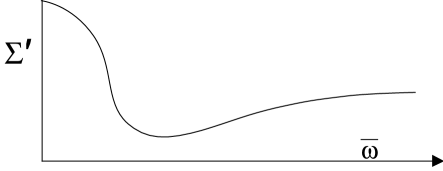
Figure 14.  : A sketch of the expected form of the real part, $\Sigma^{\prime}$, of the universal scaling function $\Sigma$ appearing in the scaling form (87) for the conductivity, as a function of $\overline{\omega}=\hbar\omega/k_{B}T$. There is a Drude-like peak from the inelastic scatterings between thermally excited carriers at $\overline{\omega}$ of order unity. At larger $\overline{\omega}$, there is a crossover to the collisionless regime where $\Sigma^{\prime}\rightarrow\Sigma(\infty)$ .

We have assumed that $\Sigma(0)>\Sigma(\infty)$, and this will be the case in the specific calculation for ${\cal S}$ discussed below. The minimum at $\omega\sim k_{B}T/\hbar$ also appears in the calculation below, but it is not clear whether that is a general feature.

It is also interesting to consider the implication of Fig 14 for $\sigma(\omega,T\rightarrow 0)$. This is illustrated in Fig 15 which plots the form of $(\hbar/Q^{2})\sigma(\omega,T\rightarrow 0)$ in $d=2$: its value at $\omega=0$ is given by $\Sigma(0)$, while for all $\omega>0$ it equals $\Sigma(\infty)$.

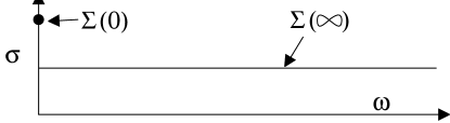
Figure 15.  : Universal form of the conductivity $\sigma(\omega,T\rightarrow 0)$ in $d=2$; the vertical scale is measured in units of $\hbar/Q^{2}$. Only the $\omega=0$ value is given by the universal number $\Sigma(0)$. For all $\omega>0$, $(\hbar/Q^{2})\sigma=\Sigma(\infty)$.

Note the difference from Fermi liquid theory, where the Drude peak becomes a delta function with non-zero weight as $T\rightarrow 0$. In the present case, the weight in the Drude-like peak vanishes like $\sim T$ as $T\rightarrow 0$, and reduces to the single point $\omega=0$ where the conductivity is given by $\Sigma(0)$.

We note that the above discussion implies results that are rather remarkable from a traditional quantum transport point of view. There have been a number of previous situations in which charge transport properties have been found to be universally related to the quantum unit of conductance, $e^{2}/h$; these include the quantized Landauer conductance of ballistic transport in one-dimensional wires, and the universal conductance fluctuations of mesoscopic metals [87]. However in all previous cases, these universal properties have arisen in a “phase-coherent” regime, i.e. they are associated with physics at scales shorter than the mean distance between inelastic scattering events between the carriers. For the case of a $d=2$ quantum critical point discussed above, the universal number $\Sigma(\infty)$ is associated with quantum coherent transport, and is therefore the analog of these earlier results. In contrast, the value of $\Sigma(0)$ is controlled by repeated inelastic scattering events, and therefore the d.c. transport is clearly in what would traditionally be identified as the “incoherent” regime. Nevertheless, we have argued above that $\Sigma(0)$ is a universal number, and the d.c. conductance remains universally related to $(Q=e)^{2}/h$.

Let us now turn to the computation of $\Sigma$ for the specific model ${\cal S}$. The $T>0$ transport properties of ${\cal S}$ in $d=2$ were considered briefly by Cha et al. [72]. They concluded that the continuum model ${\cal S}$ had $\sigma=\infty$ for all $T>0$, and that additional lattice umklapp scattering effects were needed to degrade the current carried by thermally excited carriers, and to yield a $\sigma<\infty$. However, in Section 3.3 we a found finite diffusivity $D_{s}$ for $N=3$, $d=1$ at $T>0$, and we claim that a similar result holds here for $N=2$, $d=2$. The basic point can be made quite simply by a glance at Fig 11. Note that in this $d=1$ model, the transport of momentum is indeed ballistic, and is represented by the straight line trajectories which extend for all time. However, when we consider the transport of charge, we have to follow the motion of the $N$-valued $O(N)$ index carried by each trajectory: this motion is seen in Fig 11 to be rather complicated, and was shown in Section 3.3 to be diffusive. There is thus an essential difference between momentum and charge transport when the excitations carry a $O(N)$ flavor index, and it appears to have been overlooked in Ref [72].

We will outline the recent computation of $\Sigma$ in an expansion in $\epsilon=3-d$ [63]. For small $\epsilon$ the quartic interaction, $u_{0}$, in ${\cal S}$ reaches a universal (to leading order in $\epsilon$) fixed point value [1]

$$u_{0}=\frac{24\pi^{2}}{5}\epsilon$$ (89)

in the vicinity of the quantum critical point. So the scattering of the elementary excitations, and the non-ballistic motion of the charge current, only occurs with an amplitude of order $\epsilon$. Such a weak-coupling $S$-matrix should be compared with the complementary strong-coupling $S$-matrix in (76) for $d=1$: in the latter case we had a maximal scattering situation as momentum and spin labels interchanged their mutual pairing in every collision. Also in contrast to the real-space formulation of transport taken for $d=1$ in Section 3.3, the weak-coupling situation here is best analyzed in momentum space. We wish to work with same charge eigenstates we considered in Section 3.3, and so we express the field $\Psi$ in the associated normal modes

$$\Psi({\bf x},t)=\int\frac{d^{d}k}{(2\pi)^{d}}\frac{1}{\sqrt{2\varepsilon_{k}}}\left(a_{+}({\bf k},t)e^{i{\bf k}\cdot{\bf x}}+a_{-}^{\dagger}({\bf k},t)e^{-i{\bf k}\cdot{\bf x}}\right),$$ (90)

where $\varepsilon_{k}=(k^{2}+m^{2})^{1/2}$, with $m$ a renormalized $T$-dependent mass [63]. The operators $a_{\pm}$ annihilate particles with $O(2)$ charges $\pm 1$ (in Section 3.3, where we considered $O(3)$, there were three such particles). Next, transport theory requires the momentum space distribution functions

$$f_{\lambda}({\bf k},t)=\left\langle a^{\dagger}_{\lambda}({\bf k},t)a_{\lambda}({\bf k},t)\right\rangle,$$ (91)

with $\lambda=\pm 1$, in terms of which a quantum Boltzmann equation for transport in a weakly-scattering system can be obtained [86]. We will not display the explicit form of this equation, or discuss its solution here: the reader should consult Ref [63]. That analysis leads to an explicit solution for $\Sigma$ which has the qualitative form of Fig 14. We quote quantitative results for the two limiting values [63, 78]:

$$\Sigma(0) = \frac{0.1650}{\epsilon^{2}}+\ldots$$

$$\Sigma^{\prime}(\overline{\omega}\rightarrow\infty) = \frac{2^{1-2d}\pi^{1-d/2}}{d\Gamma(d/2)}\left(1+{\cal O}(\epsilon^{2})\right)\overline{\omega}^{1-\epsilon}$$ (92)

to leading order in $\epsilon$. Notice the singular $\epsilon$ dependence of the first result: this is signal of a “boundary layer” in $\Sigma$ of width $\omega\sim\epsilon^{2}T$ which constitutes the “Drude peak” of Fig 14. This boundary layer explicitly demonstrates a claim made in Section 1: the operations of expansion in $\epsilon$ and of analytic continuation in $\omega$ do not commute. The structure of the higher-order corrections to the first result in (92) is quite complex, and was generally discussed in Ref [8]. For the superfluid insulator transition in $d=2$ with $Q=2e$, (92) implies a universal d.c. conductivity

$$\sigma(0)=2\pi\Sigma(0)\frac{4e^{2}}{h}\approx 1.037\frac{4e^{2}}{h}$$ (93)

This result is remarkably close to the value, $4e^{2}/h$ (argued [75, 76] to be related to self-duality), and to the results of many experiments [66]. Indeed, it was conjectured in Ref [63] that $2\pi\Sigma(0)=1$ exactly for $N=2$ in $d=2$. Definitively establishing this self-duality however requires techniques other than expansion in $\epsilon=3-d$, or $1/N$, as it is only possible precisely at $d=2$, $N=2$. Finding such techniques is an important challenge for future work.

5 Conclusion

We have reviewed the universal, non-zero temperature dynamic properties of the CQFT ${\cal S}$ for a number of representative cases, and discussed their experimental implications. Among the cases omitted, there are some that show phenomena qualitatively different from those discussed here:
(i) The case $N=2$, $d=1$ has a line of critical points and a Kosterlitz-Thouless end point at $T=0$. Its paramagnetic phase is similar to the $N=3$, $d=1$ model discussed in Section 3.3.
(ii) For $d>3$ there is violation of hyperscaling, which leads to explicit dependence of finite $T$ behavior on the bare value of $u_{0}$ and qualitatively different crossovers [8].

- [1] E. Brezin, J.C. Le Guillou and J. Zinn-Justin in Phase Transitions and Critical Phenomena , vol. 6, C. Domb and M.S. Green eds., Academic Press, London (1976).
- [2] Quantum Field Theory and Critical Phenomena by J. Zinn-Justin, Oxford University Press, Oxford (1993).
- [3] S. Sachdev in the Proceedings of the 19th IUPAP International Conference on Statistical Physics, Xiamen, China, July 31 - August 4 1995, edited by B.-L. Hao, World Scientific, Singapore (1996); Report No. cond-mat/9508080.
- [4] J.A. Hertz, Phys. Rev. B 14, 525 (1976).
- [5] M.A. Continentino, Phys. Rep. 239, 179 (1994).
- [6] S. Sachdev and J. Ye, Phys. Rev. Lett. 69, 2411 (1992).
- [7] A.V. Chubukov, S. Sachdev and J. Ye, Phys. Rev. B 49, 11919 (1994).
- [8] S. Sachdev, Phys. Rev. B 55, 142 (1997).
- [9] J.B. Kogut, Rev. Mod. Phys. 51, 659 (1979).
- [10] E. Lieb, T. Schultz, and D. Mattis, Ann. of Phys. 16, 406 (1961).
- [11] P. Pfeuty, Ann. of Phys. 57, 79 (1970).
- [12] Statistical Field Theory by C. Itzykson and J.-M. Drouffe, Cambridge University Press, Cambridge (1989).
- [13] J.L. Cardy, J. Phys. A 17, L385 (1984).
- [14] B.M. McCoy, Phys. Rev. 173, 531 (1968).
- [15] E. Barouch and B.M. McCoy, Phys. Rev. A 3, 786 (1971); B.M. McCoy et al., Phys. Rev. A 4, 2331 (1971).
- [16] S. Sachdev, Nucl. Phys. B 464, 576 (1996)
- [17] S. Sachdev and A.P. Young, Phys. Rev. Lett. 78, 2220 (1997).
- [18] Quantum Inverse Scattering Method and Correlation Functions by V.E. Korepin, N.M. Bogoliubov, and A.G. Izergin, Cambridge University Press, Cambridge (1993).
- [19] A. Leclair, F. Lesage, H. Saleur, and S. Sachdev, Nucl. Phys. B 482, 579 (1996).
- [20] H.W. Capel and J.H.H. Perk, Physica 87A, 211 (1977); J.H.H. Perk et al. Physica 123A, 1 (1984).
- [21] S. Chakravarty, B.I. Halperin, and D.R. Nelson, Phys. Rev. B 39, 2344 (1989).
- [22] L.B. Keldysh, Zh. Eksp. Teor. Fiz. 47, 1515 (1964) [Sov. Phys. JETP 20, 235 (1965)]; P. Danielewicz, Ann. of Phys. 152, 239 (1984).
- [23] A similar relaxation function was also obtained in a phenomenological analysis of related models by exponentiating a short-time expansion which ignored collisions in K. Maki Phys. Rev. B 24 335 (1981) and F. Devreux and J.P. Boucher J. de Physique 48, 1663 (1987)
- [24] R.J. Glauber, J. Math. Phys. 4, 294 (1963).
- [25] J.L. Cardy and G. Mussardo, Nucl. Phys. B 340, 387 (1990); V.P. Yurov and Al.B. Zamalodchikov, Int. J. Mod. Phys. A 6, 3419 (1991).
- [26] O. Babelon and D. Bernard, Physics Letters. B 288, 113 (1992).
- [27] S. Sachdev, T. Senthil, and R. Shankar, Phys. Rev. B 50, 258 (1994).
- [28] P.C. Hohenberg and B.I. Halperin, Rev. Mod. Phys. 49, 435 (1977).
- [29] S. Sachdev, Phys. Rev. B 50, 13006 (1994).
- [30] M. Takigawa et al., Phys. Rev. Lett. 76, 4612 (1996).
- [31] O. A. Starykh, R. R. P. Singh and A. W. Sandvik, Phys. Rev. Lett. 78, 539 (1997).
- [32] M. Azuma et al. Phys. Rev. Lett. 73, 3463 (1994).
- [33] S. Das Sarma, S. Sachdev, and L. Zheng, Report no. cond-mat/9701142.
- [34] V. Pellegrini et al., Phys. Rev. Lett. 78, 310 (1997); L. Zheng, R.J. Radtke, and S. Das Sarma, Phys. Rev. Lett. 78, 2453 (1997).
- [35] A.M. Polyakov, Phys. Lett. B 59, 87 (1975).
- [36] Th. Joliceour and O. Golinelli, Phys. Rev. B 50, 9265 (1994).
- [37] M. Luscher, Phys. Lett. 118B, 391 (1982).
- [38] S. Sachdev and K. Damle, Phys. Rev. Lett. 78, 943 (1997).
- [39] K. Damle and S. Sachdev, in preparation.
- [40] A.B. Zamalodchikov and A.B. Zamalodchikov, Ann. of Phys. 120, 253 (1979).
- [41] D.W. Jepsen, J. Math. Phys. 6, 405 (1965).
- [42] J.L. Lebowitz and J.K. Percus, Phys. Rev. 188, 487 (1969).
- [43] M. Takigawa et al., Phys. Rev. Lett. 76, 2173 (1996).
- [44] T. Shimizu et al., Phys. Rev. B 52, R9835 (1995).
- [45] A Quantum-critical Trio, by S. Sachdev in Strongly Correlated Magnetic and Superconducting Systems, Proceedings of the El Escorial Summer School, 15-19 July, 1996, G. Sierra and M. Martin-Delgado eds., Springer Verlag, to be published.
- [46] S. Tyc and B.I. Halperin, Phys. Rev. B 42, 2096 (1990).
- [47] A.V. Chubukov and S. Sachdev, Phys. Rev. Lett. 71, 169 (1993).
- [48] T. Imai et al. Phys. Rev. Lett. 70, 1002 (1993)
- [49] T. Imai et al. Phys. Rev. Lett. 71, 1254 (1993).
- [50] A.V. Chubukov, S. Sachdev, and A. Sokol, Phys. Rev. B 49, 9052 (1994).
- [51] A. Sokol, R.L. Glenister, and R.R.P. Singh, Phys. Rev. Lett. 72, 1549 (1994).
- [52] N. Elstner, R.L. Glenister, R.R.P. Singh, and A. Sokol: Phys. Rev. B 51, 8984 (1995).
- [53] M. Greven et al., Phys. Rev. Lett. 72, 1096 (1994); Z. Phys. B 96, 465 (1995).
- [54] D.F. McMorrow, private communication.
- [55] J. M. Tranquada et al., Phys. Rev. B 40, 4503 (1989); A. J. Millis and H. Monien, Phys. Rev. Lett. 70, 2810 (1993); Phys. Rev. B 50, 16606 (1994).
- [56] A.W. Sandvik and D.J. Scalapino, Phys. Rev. Lett. 72, 2777 (1994); A. W. Sandvik, A.V. Chubukov and S. Sachdev, Phys. Rev. B, 51, 16483 (1995).
- [57] A.W. Sandvik, R.R.P. Singh and A. Sokol, unpublished.
- [58] K. Hida, J. Phys. Soc. Japan 61, 1013 (1992); M.P. Gelfand, Phys. Rev. B 53, 11309 (1996); W.H. Zheng, Report no. cond-mat/9701214; M.P. Gelfand, Z. Weihong, C.J. Hamer and J. Oitmaa, Report no. cond-mat/9705201.
- [59] M. Troyer, M. Imada and K. Ueda, Report no. cond-mat/9702077.
- [60] S. Sachdev and N. Read, Phys. Rev. Lett. 77, 4800 (1996); N. Read and S. Sachdev, Phys. Rev. B 42, 4568 (1990).
- [61] B. Normand and T.M. Rice, Phys. Rev. B 54, 7180 (1996); cond-mat/9701202.
- [62] M. Troyer, M.E. Zhitomirsky and K. Ueda, Phys. Rev. B 55, R6117 (1997).
- [63] K. Damle and S. Sachdev, submitted to Phys. Rev. B; Report no. cond-mat/9705206.
- [64] M.P.A. Fisher, P.B. Weichmann, G. Grinstein, and D.S. Fisher, Phys. Rev. B 40, 546 (1989).
- [65] A.F. Hebard in Strongly Correlated Electronic Materials (The Los Alamos Symposium 1993), K.S. Bedell, Z. Wang, D.E. Meltzer, and E. Abrahams eds, Addison Wesley, Reading MA (1994), p. 251, and references therein.
- [66] Y Liu and A.M. Goldman, Mod. Phys. Lett. B 8, 277 (1994) and references therein.
- [67] H.S.J. van der Zant et al., Phys. Rev. Lett. 69, 2971 (1992).
- [68] S.L. Sondhi, S.M. Girvin, J.P. Carini and D. Shahar, Rev. Mod. Phys. 69, 315 (1997) and references therein.
- [69] S. Das Sarma in Perspectives in Quantum Hall Effects, S. Das Sarma and A. Pinczuk eds, Wiley, New York (1997), p. 1, and references therein.
- [70] S. Kivelson, D.H. Lee and S.C. Zhang, Phys. Rev. B 46, 2223 (1992).
- [71] M.P.A. Fisher, G. Grinstein, and S.M. Girvin, Phys. Rev. Lett. 64, 587 (1990).
- [72] M.-C. Cha, M.P.A. Fisher, S.M. Girvin, Mats Wallin, and A.P. Young, Phys. Rev. B 44, 6883 (1991).
- [73] S. Sachdev, Z. Phys. B 94, 469 (1994).
- [74] M. Wallin, E.S. Sorensen, S.M. Girvin, and A.P. Young, Phys. Rev. B 49, 12115 (1994).
- [75] M.P.A. Fisher, Phys. Rev. Lett. 65, 923 (1990).
- [76] X.G. Wen and A. Zee, Int. J. Mod. Phys. B4, 437 (1990).
- [77] A.P. Kampf and G.T. Zimanyi, Phys. Rev. B 47, 279 (1993).
- [78] R. Fazio and D. Zappala, Phys. Rev. B 53, R8883 (1996).
- [79] I.F. Herbut, Report no. cond-mat/9704134.
- [80] X.G. Wen and Y.S. Wu, Phys. Rev. Lett. 70, 1501 (1993).
- [81] W. Chen, M.P.A. Fisher, and Y.S. Wu, Phys. Rev. B 48, 13749 (1993).
- [82] K. Runge, Phys. Rev. B 45, 13136 (1992).
- [83] E.S. Sorensen, M. Wallin, S.M. Girvin, and A.P. Young, Phys. Rev. Lett. 69, 828 (1992).
- [84] M. Makivic, N. Trivedi, and S. Ullah, Phys. Rev. Lett 71, 2307 (1993).
- [85] G.G. Batrouni, B. Larson, R.T. Scalettar, J. Tobochnik, and J. Wang, Phys. Rev. B 48, 9628 (1993).
- [86] L.P. Kadanoff and G. Baym, Quantum Statistical Mechanics, Benjamin, New York (1962).
- [87] Mesoscopic Phenomena in Solids, edited by B.L. Altshuler, P.A. Lee and R.A. Webb, North Holland, Amsterdam (1991) and references therein.