Abstract

Interface equations are derived for both binary diffusive and binary fluid systems subjected to non-equilibrium conditions, starting from the coarse-grained (mesoscopic) models. The equations are used to describe thermo-capillary motion of a droplet in both purely diffusive and fluid cases, and the results are compared with numerical simulations. A mesoscopic chemical potential shift, owing to the temperature gradient, and associated mesoscopic corrections involved in droplet motion are elucidated.

keywords: interface equations, thermocapillary motion, capillarity

I Introduction

The study of interfacial dynamics in multi-phase systems has been a topic of considerable interest in recent years. A wide range of phenomena such as solidification, viscous fingering, droplet migration, spinodal decomposition and fracture all involve, in one way or another, a description of interfacial motion. Often analysis of these and related phenomena is performed at the macroscopic level, using, for example, hydrodynamic equations supplemented by appropriate phenomenological boundary conditions. Macroscopic interface equations are exceptionally useful both conceptually and computationally in that bulk degrees of freedom are eliminated; computationally the cost is the required careful tracking of the interface position and shape. Some examples of their application are included in Ref. [1] and citations therein.

The macroscopic approach, while valuable in its own domain, has natural limitations. The most obvious lie in situations in which the scale of structures is not sufficiently larger than the physical interfacial thickness, which can grow to several molecular length scales not too far from criticality, for example. Phenomena such as coalescence ultimately run macroscopic approaches to their limits, although ad hoc but reasonable methods are often available for resolving singularities having to do with infinitely sharp interfaces. In addition, one may wonder whether macroscopic boundary conditions may require correction in situations which strain the assumptions.

Derivations of macroscopic interface equations from more microscopic starting points can be extremely useful in illuminating just what assumptions are necessary and the potential limitations. Indeed considerable progress has been made in this regard beginning from a coarse-grained or mesoscopic level. [2] However, the interfacial response to non-equilibrium perturbations or inhomogeneities such as an imposed small thermal gradient, can pose interesting challenges. In this paper, we develop interface equations starting from mesoscopic (coarse-grained) models for both purely diffusive binary systems and binary systems with hydrodynamic interactions, subjected to small non-equilibrium perturbations. Using this approach, we investigate as an example, thermo-capillary driven motion of a droplet in both binary diffusive and binary fluid systems in an imposed temperature gradient. Note that motion of a droplet in the hydrodynamic case has been well explored by the use of macroscopic techniques [3, 4, 5], while diffusion driven thermo-capillary motion has not been received much attention in the literature [6]. Thus, to the best of our knowledge, our modeling approach provides a first detailed comparison for the droplet motion in these two distinctly different cases. Furthermore, in addition to reproducing the results consistent with macroscopic hydrodynamics, the coarse-grained modeling approach also provides a means to investigate mesoscopic corrections associated with finite interfacial thickness. This feature may prove useful in understanding interfacial dynamics at mesoscopic length scales.

The remainder of this paper is laid out as follows. In the next Section we introduce the notation and briefly review the coarse-grained models we will consider along with the relevant equilibrium features. Section III deals with the introduction of the types of non-equilibrium considered here and with the effect on a single flat interface. Section IV contains the derivation of the macroscopic interface equations and mesoscopic corrections in both the fluid and diffusive cases.

II Models

We begin with the d-dimensional coarse-grained (mesoscopic) binary fluid and binary diffusive models which are commonly referred to as the Model-H and Model-B in the literature [7]. These traditional models have been extensively used to investigate critical fluctuations in binary systems. However, the usefulness of such models for regions well below the critical point is still being established, by, for example, demonstrating that in particular limits well established macroscopic results are reproduced. [8] This remains a focus in this paper. One advantage of this type of modeling is that the physics of capillarity is naturally built-in as opposed to being introduced through boundary conditions in macroscopic techniques.

A Hydrodynamic Model

The coarse-grained model is defined by a conserved order parameter $\phi$ (e.g., concentration of one of the phases) whose evolution is given by

$$\frac{\partial\phi(\vec{r},t)}{\partial t}+\vec{\nabla}\cdot(\phi\vec{v})=\nabla^{2}\mu(\vec{r},t)$$ (1)

where $\mu=(\frac{\delta F}{\delta\phi})$ is the appropriate chemical potential given by the functional derivative of the Helmholtz free energy $F$. The fluid velocity $\vec{v}(\vec{r},t)$ satisfies a modified Navier-Stokes equation,[7, 8]

$$\rho\frac{\partial\vec{v}}{\partial t}=\eta\nabla^{2}\vec{v}-\vec{\nabla}P+\mu\vec{\nabla}\phi$$ (2)

where $P$ is the pressure, $\eta$ and $\rho$ are viscosity and density respectively, which are assumed to be fixed and equal for both phases for simplicity. Equations (1) and (2) along with the incompressibility condition, $\vec{\nabla}\cdot\vec{v}=0$, completely specify the hydrodynamic model with the following three boundary conditions: (B1) $\partial\mu/\partial n=0$; (B2) $\partial\phi/\partial n=0$ and, for example, (B3) $\vec{v}=0$ on the boundary. Here $\partial/\partial n$ corresponds to the normal derivative at the system boundary. The condition B1 preserves the global conservation of order parameter $\phi$, B2 is the natural boundary condition which demands smoothness of $\phi$ at the edges, and B3 enforces “no-slip,” with other possibilities easily included. Note that our interest here is to address small Reynolds numbers ($Re$) and, hence, the nonlinear convective terms have been dropped in the velocity equation (2).

B Diffusive Model

Model-B is in turn specified by evolution equation

$$\frac{\partial\phi(\vec{r},t)}{\partial t}=\nabla^{2}\mu$$ (3)

with boundary conditions B1 and B2 mentioned above. One may view this as the diffusion dominated limit of Eq. (1) where the fluid velocity is neglected. This is a version of Cahn-Hilliard model for binary diffusive systems used to study phase separation [9].

The mean-field level equilibrium properties of the two coexisting phases are characterized by the local Helmholtz free energy density which, for systems of interest, we take as a polynomial function

$$f=\sum_{n>0}\frac{\alpha_{n}}{n}\phi^{n}$$ (4)

with the coefficients $\alpha_{n}$ depending smoothly on physical fields such as the temperature chosen such that the system is within the two phase regime. Although it is not essential we will generally assume a scaling equation of state (see below). The equilibrium properties depend on the local temperature $T$ and other field variables that determine the $\alpha_{n}$. For example, taking $\alpha_{2}=-\tau$, where $\tau>0$ depending linearly on the temperature [$\tau=(T_{c}-T)/T_{c}$ with $T_{c}$ being the mean field critical temperature], and $\alpha_{4}=1$ with all other $\alpha_{n}=0$, we have the usual double-well Landau free energy, which will serve as our “standard model.” The (Helmholtz) free energy functional for this case is given by

$$F\{\phi\}=\int\{\ell^{2}\frac{(\nabla\phi)^{2}}{2}+f(\phi)\}d^{d}r=\int\{\ell^{2}\frac{(\nabla\phi)^{2}}{2}-{\tau}\frac{\phi^{2}}{2}+\frac{\phi^{4}}{4}\}d^{d}r,$$ (5)

where we assume the mesoscopic length $\ell$ is typically of the order of several molecular spacings some distance below the critical point. This length characterizes spatial variations of the order parameter and consequently sets the interfacial thickness. The chemical potential $\mu$ is given by

$$\mu(\vec{r},t)=-\ell^{2}\nabla^{2}\phi+\frac{\partial f}{\partial\phi}=-\ell^{2}\nabla^{2}\phi-\tau\phi+\phi^{3}.$$ (6)

Note that our standard model corresponds to a symmetric situation with equilibrium phase values $\phi_{eq}=\pm\sqrt{\tau}$; the coexistence curve is symmetric and, for example, response functions and other bulk properties are identical in the coexisting phases. When the system is in equilibrium, a flat interface with normal along $x$ has the well-known profile (exact within this mean-field level in an infinite system),

$$\phi(x)=\phi_{eq}{\tanh}[\frac{x-x_{0}}{\sqrt{2}\xi}],$$ (7)

where $x_{0}$ is the location of the interface and $\xi=\ell/\sqrt{\tau}$ is the thermal correlation length (see, e.g., Ref. [9, 10] for details of this analysis). Note that the profile takes values $\pm\phi_{eq}$ at $x=\pm\infty$ respectively. In a finite system this serves as a good approximation for the profile so long as the system size is much larger than the interfacial thickness $\xi$. We will assume more generally scaling behavior for the order parameter profile, $\phi(x)=\phi_{eq}h(\frac{x-x_{0}}{\xi}),$ with $h(y)\rightarrow\pm 1$ as $y\rightarrow\pm\infty$. Such behavior will follow from a scaling equation of state determined by $f(\phi)$ [11, 10], or quite generally with the identification of $\xi$ with $\ell$. The profile given in Eq. (7) satisfies Eq. (6) with constant $\mu$. Note that $\mu=0$ for a symmetric system at two-phase coexistence and for the above interfacial profile. Using these features, and a scaling form for the profile, it is straightforward to show [12, 10] that the surface tension $\sigma$ is given by $\sigma(\tau)=\ell^{2}\int(\frac{\partial\phi}{\partial x})^{2}dx=\frac{e_{1}\ell^{2}\phi_{eq}^{2}}{\xi}$, where $e_{1}$ is a non-universal constant depending on details of the profile $h(x)$ and taking the value $2\sqrt{2}/3$ in the standard $\phi^{4}$-case. Note that the surface tension depends on the temperature (and ultimately on the local temperature) through the $\phi_{eq}$ and $\xi$. Also, note that the analysis can be extended by choosing the coefficients $\alpha_{n}$ such that the macroscopic limit (i.e., formally, $\ell\rightarrow 0$) of $\sigma$ exists. Physically the macroscopic limit obtains when the scale of any structures greatly exceeds the interfacial thickness, which is of order $\xi\sim\ell$. Specifically, for the above $\phi^{4}$-symmetric model, the choice $\alpha_{2}=\tau_{0}/\ell^{2}$ and $\alpha_{4}=u_{0}/\ell^{2}$ (with $u_{0}=1$ for simplicity) ensures the finiteness of $\sigma$ as well as the bulk order parameter values in the macroscopic or sharp interface limit, $\ell\rightarrow 0$. For specificity we will use the symmetric $\phi^{4}$ model described above. The first equality in Eq. (6) is general; we will use it and indicate below which features are model dependent.

III Introducing driving terms

When the $\alpha_{n}$ are spatially uniform and chosen such that the system is on the bulk phase boundary, the system can evolve to a simple equilibrium state with a single homogeneous phase or a two-phase equilibrium with flat interface and volume fractions chosen according to the overall order parameter. Considerable progress has been made in the study of kinetics of the approach to equilibrium and of phase separation in such cases; see, e.g.,Refs. [9, 13]. Macroscopic interface equations have been derived from the coarse grained level in order to to explore the physics of phase ordering kinetics [2, 14]. However, when one or more of the $\alpha_{n}$ has a small spatial variation, the situation is somewhat different.

In such a situation, the system may be able to reach an inhomogeneous equilibrium state depending on the nature of the variation and the boundary conditions. For example, in a closed system, a fluid in a gravitational field reaches an equilibrium state with a spatially varying density. However, in a sufficiently large system, such an inhomogeneity can yield interesting dynamical evolution long before the walls come into play. [15] An example which produces quasi-stationary states is that of capillarity driven droplet motion in a temperature gradient. [8]. Here, in the simplest case, a droplet drifts toward the ‘hot’ side with approximately steady state motion until reaching the vicinity of the system boundary. In this approximate steady state, the system is spatially non-uniform, but close to local equilibrium everywhere. In such cases, the interfacial dynamics are influenced by the spatial variation in the surface tension resulting from the spatial dependence of the $\alpha_{n}$. Our interest here is to address this spatially inhomogeneous situation and present an approach for deriving reduced equations that describe the interfacial dynamics.

For specificity we consider the following spatial dependence in the standard example mentioned above: $\tau(x)=-\alpha_{2}(x)=\tau_{0}-\beta x>0$, $\alpha_{4}=1,$ and all other $\alpha_{n}=0$ in the free energy given by Eq. (4). This situation corresponds to imposing a temperature gradient on the system along $x$ direction with the two ends kept at temperatures corresponding to $\tau_{0}$ and $\tau_{0}-\beta L_{x}$ where $L_{x}$ is the size of the system along $x$. We restrict ourselves to temperatures slowly varying over the correlation length so that $\beta\xi<<1$. This is easily satisfied experimentally, and our analysis remains valid even for temperature gradients large by experimental standards. [8] Furthermore we consider only the situation in which the entire system is in the two-phase region. Thermocapillary phenomena associated with such type of thermal gradients have been numerically investigated recently in Refs. [8, 16, 17, 6]. Note that the spatial variation and hence, the temperature field, is fixed, corresponding to large thermal conductivity of the medium. Generalizations to treating the temperature field as an active dynamical variable are possible and will be treated elsewhere.

Before considering the evolution of a complicated interface, it is useful to examine the properties of a stationary flat interface with its normal along $x$ in a thermal gradient. In such steady state, which exists for the case of conserved order parameter, $\partial\phi/\partial t=0$ and $v=0$. Hence following from Eq. (1), $\mu$ should be a constant since $\partial\mu/\partial n=0$ at the system boundaries. However, the steady state profile $\phi(x)$ (consistent with a non-vanishing, constant value of $\mu$) is a combination of two ramps as shown from direct simulations of the coarse grained model in Fig. 1. Below we will use a local equilibrium approximant which describes the ramp profile very well. The location $x_{0}$ of the interface depends on the initial order parameter content in the system. It is important to recognize that for conserved order parameter the profile of Fig. 1 represents an equilibrium state, while for nonconserved order parameter the ‘kink’ quite generally moves with constant velocity toward the hot side as order parameter is converted in such a way as to reduce the total free energy. [18]

For the present (conserved) case, by assuming that the interface at $x=0$ is at local equilibrium corresponding to the temperature $\tau(x=0)$, one can obtain $\mu$ to first order in the gradient $\beta$ as follows. First, to simplify the algebra we rewrite $\tau(x)=m(x)^{2}$ with $m(x)=m_{0}(1-bx)$. To $\cal{O}(\beta)$ there is no change if we identify $b=\beta/2$ and $m_{0}=1$. For simplicity we set $\ell=1$ and have $\mu=-\frac{d^{2}\phi}{dx^{2}}-m^{2}(x)\phi+\phi^{3}.$ Following Ref. [18] we remove the local equilibrium order parameter and make a non-linear transformation defining $\phi(x)=m(x)\eta(z(x)).$ We set the function $z(x)$ by requiring that the resulting differential equation for $\eta(z)$ has unity for the coefficient of $d^{2}\eta/dz^{2}$. One finds, then, that $z(x)=m_{0}(x-bx^{2}/2)$ and

$$\frac{\mu}{m(x)^{3}}=-\frac{d^{2}\eta}{dz^{2}}-\eta+\eta^{3}+(3bm_{0}/m^{2})\frac{d\eta}{dz}$$ (8)

This procedure effectively isolates the explicit dependence on the temperature gradient $b\propto\beta$. Now one can perform an order-by-order analysis, writing $\eta=\eta_{0}(z)+b\eta_{1}(z)+\dots$ and $\mu=\mu_{0}+b\mu_{1}+\dots$. At ${\cal O}(b^{0})$ we have

$$\frac{\mu_{0}}{m_{0}^{3}}=0=-\frac{d^{2}\eta_{0}}{dz^{2}}-\eta_{0}+\eta_{0}^{3}$$ (9)

with, as expected, $\eta_{0}=\tanh(z/\sqrt{2})$. The function $\phi_{0}=m(x)\eta_{0}(z)$ corresponds to the local equilibrium ramp and is an excellent numerical approximation. In fact, if plotted on the same scale as the simulation result in Fig. 1, there would be virtually no visible difference.

At ${\cal O}(b)$ we have

$$\frac{\mu_{1}}{m_{0}^{3}}={\cal L}\eta_{1}+\frac{3}{m_{0}}\frac{d\phi_{0}}{dz}$$ (10)

where the operator ${\cal L}=-d^{2}/dz^{2}-1+3\eta_{0}^{2}$ is recognized as the fluctuation operator for the $\phi^{4}$ theory, and $d\eta_{0}/dz$ is the so-called ‘translation mode’ (see, e.g., Ref. [10]). Multiplying through by $d\eta_{0}/dz$, and recalling that ${\cal L}d\eta_{0}/dz=0$, one finds the chemical potential shift

$$\mu_{1}=\sqrt{2}m_{0}^{2}b=\frac{\beta\ell}{\sqrt{2}}.$$ (11)

In the last equality we have reintroduced the mesoscopic length $\ell$ and have returned to the original definition of the temperature gradient $\beta$.

The mesoscopic shift in chemical potential, $\mu_{m}=\pm\mu_{1},$ is proportional to the mesoscopic length scale $\ell$. Also note that $\mu_{m}>0(<0)$ depending on whether the $\phi>0(<0)$ phase is near the hot end. Physically the chemical potential shift (from the coexistence value $\mu=0$) is proportional to the temperature difference across the interfacial region, which is generally small. For the profile shown in Fig. 1, the chemical potential $\mu$ evaluated from Eq. (6) is negative, as shown in the inset. For the $\phi^{4}$ model, using the parameters of Fig. 1, one finds $|\mu_{m}|=0.004/\sqrt{2}\simeq 0.00283$ in excellent agreement with the direct simulation. At the time shown in Fig. 1, the interface hasn’t quite equilibrated in this diffusive system. Small order parameter changes in the evolution are emphasized in the chemical potential. For complete equilibration, global diffusion is required. Simulations on smaller systems and in one-dimension reveal, more rapidly, a constant chemical potential. Recall that the homogeneous case having $\tau=\tau_{0}=\mbox{const}$ has $\mu=0$.

The above analysis arriving at the leading behavior of a flat interface, i.e., $\phi~{}=~{}\sqrt{\tau(x)}\tanh(z(x))$ can be viewed as taking the sharp interface limit in which the fast variations of the order parameter along the normal at the interface are considered. Note that the slow variation associated with the temperature field is effectively ignored while integrating though the interface. Furthermore, if the normal to the interface is tilted by an angle $\theta$ with respect to the $x-$axis (the direction of temperature variation) one repeats the above analysis using $\phi=m(x^{\prime}\cos\theta)\tanh(z(x^{\prime}))$ where $x^{\prime}$ is the coordinate in the normal direction. Everything goes through as above with the mesoscopic correction becoming $\mu_{1}\cos(\theta)$ where $\mu_{1}$ is given in Eq. (11). Below the calculation will be slightly modified to deal with a gently curving interface.

Numerical simulations, such as shown in Fig. 1, confirm that the models exhibit this shift, supporting the local equilibrium picture of interface in an inhomogeneous, slowly varying temperature field. As noted, a single two-phase interface, owing to the conservation of order parameter, can achieve an equilibrium state in a large, finite system. A slab consisting of a combination of two opposite interfaces, i.e., a kink-antikink, cannot. In fact the mesoscopic shift in chemical potential alone drives the slab to the hotter side. This phenomenon will be addressed elsewhere [19].

IV Interface equations

We now consider a gently curved interface in the coarse-grained modeling and derive equations for the evolution of the interface. We restrict ourselves to two dimensions for simplicity since appropriate generalizations for higher dimensions can be made straightforwardly.

To determine the effect of an applied gradient, we first assume that locally the interface is flat and is in local equilibrium with $x$ variation replaced by variation along the normal direction. The second assumption is that the interfacial motion arises from local quasi-stationary evolution of the order parameter $\phi(\vec{r},t)=\phi(\vec{r}-\vec{V}t)$. In particular, the evolution of the interface at any point $s$ is characterized by the normal velocity $\vec{V}(s)\cdot\hat{n}$, where $\hat{n}$ is a unit normal (pointing from the ‘minus’ phase to the ‘plus’ phase). This means that order parameter or fluid flow along the tangential direction at any point on the interface do not contribute to the evolution of the interface. The equations for diffusive and fluid cases differ since the mechanisms for the interfacial motion are different. Interface equations in the absence of imposed gradients have been well studied in literature [14]; our interest here is to extend the derivations and applicability of such equations to inhomogeneous perturbations which can, for example, drive steady state behavior.

A Diffusive case

Eq. (3) describing the diffusive dynamics can be inverted (see, e.g., Ref. [14]) using the assumption of local quasi-stationarity :

$$\int d^{d}r^{\prime}G(\vec{r}-\vec{r}^{\prime})\frac{\partial\phi(\vec{r}^{\prime},t)}{\partial t}=-\mu(\vec{r},t)+\lambda(t),$$ (12)

where $G$ is the Green’s function for the Laplacian satisfying $-\nabla^{2}G(\vec{r}-\vec{r^{\prime}})=\delta(\vec{r}-\vec{r^{\prime}}).$ The function $\lambda$ preserves the order parameter conservation and satisfies $\nabla^{2}\lambda=0$ with zero-gradient boundary condition as does $\mu$. One may view $\lambda$ as the change in chemical potential due to the presence of complicated interfaces in the system. The idea is to derive an equation for the interfacial motion starting from Eq. (12) by integrating the fast variation of $\phi$ along the normal at the interface. A separation of length scales allows one to take sharp interface limit in which the radius of curvature is much greater than the interface thickness; an alternative procedure for organizing corrections has been used to derive interfacial dynamics in a driven diffusive system. [20] These methods allow, however, a significant variation of temperature over the scale of a droplet.

First, the local quasi-stationarity assumption allows us to replace $\partial\phi/\partial t$ by $-\vec{V}\cdot\vec{\nabla}{\phi}$. Since the normal variation of $\phi$ at the interface dominates, we approximate it further by $-V_{n}\partial\phi/\partial n$ at the interface with $V_{n}$ being the velocity along the normal. Second, we multiply Eq. (12) on both sides by $\partial\phi/\partial n$ and then take the sharp interface limit. At any point $s$ on the interface, by ignoring the slow tangential variation of $\phi$ along the interface, we can write

$$\mu\partial\phi/\partial n\approx[-\ell^{2}\frac{\partial^{2}\phi}{\partial^{2}n}-\tau(x)\phi+\phi^{3}]\frac{\partial\phi}{\partial n}-\ell^{2}\kappa(s)(\frac{\partial\phi}{\partial n})^{2}\ \ ,$$ (13)

where $\kappa$ is the curvature. On integration through the interface, the first term in the above is exactly the equation we have for the flat interface. Hence in the sharp interface limit the first term yields the mesoscopic correction, $\mu_{m}(\hat{n}\cdot\hat{x})$, as discussed above, while the second term gives the surface tension multiplied by the local curvature, $\kappa(s)$. With these approximations, the following integral equation results for the normal velocity at the interface

$$\int_{I}ds^{\prime}G(s|s^{\prime})\Delta(s)\Delta(s^{\prime})V_{n}(s^{\prime})=\sigma(s)\kappa(s)-\mu_{m}(\hat{n}\cdot\hat{x})\Delta(s)-\lambda(t)\Delta(s),$$ (14)

where $G(s|s^{\prime})=G(\vec{r}(s)-\vec{r}(s^{\prime}))$, $\sigma(s)$ is the surface tension and $s$ and $s^{\prime}$ are points parameterized by the arc length along the interface, $I$. In the above equation tangential variations in the miscibility gap $\Delta(s)$ give rise to to terms in the interface velocity which are higher order in the temperature gradient $\beta$. The same result could be obtained without pausing to find explicitly the mesocsopic correction to the chemical potential. Since Eq. (12) will be projected onto the interface by action of $\partial\phi/\partial n$, one may use Eq. (13) with the “inner approximation” $\phi\simeq\phi^{eq}_{I}\tanh(n/\sqrt{2}\xi_{I})$, where the subscript $I$ indicates the interface location. (Of course, the form of the inner approximation is justified by the systematic analysis leading to the mesoscopic correction.) In this paper we restrict ourselves to leading order in $\beta$; hence we set $\Delta(s)=\Delta$ and obtain

$$\int_{I}ds^{\prime}G(s|s^{\prime})V_{n}(s^{\prime})=\frac{\sigma(s)\kappa(s)}{\Delta^{2}}-\frac{(\hat{n}\cdot\hat{x})\mu_{m}+\lambda(t)}{\Delta}.$$ (15)

Then the time-dependent Lagrange multiplier $\lambda(t)$ is determined as part of the solution guaranteeing conservation of the order parameter as specified, in the macroscopic limit, by the vanishing of the surface integral,

$$\int_{I}V_{n}(s)ds=0.$$ (16)

The above two equations specify the evolution of a complicated interface in the 2D diffusive model, including the leading mesoscopic correction. They can be used, for example, to study the evolution of droplets as well as other structures and interfacial instabilities. [21] Such equations, without the mesoscopic term, have been derived at the macroscopic level and used in the literature to study a variety of problems such as interfacial growth in an anisotropic Hele-Shaw cell [22].

The interface equations can be used to study the evolution of complicated interfacial shapes in general. Here we use them to study thermocapillary response of a spherical droplet of radius $R$ in $d$-dimensions to a small thermal gradient. The curvature $\kappa(s)$ at any point $s$ in this case is simply given by $\kappa(s)=(d-1)/R$, and the integration over $s^{\prime}$ in Eq. (15) is carried over a d-dimensional sphere. Note that in the absence of a gradient the droplet remains stationary since, $\sigma(s)=\sigma$ and $\mu_{m}=0$. As a result $\lambda$ is a constant and takes a value $\lambda=\lambda_{0}=\sigma(d-1)/(R\Delta)$. This is immediately recognized as the required shift in the chemical potential of the system off bulk phase coexistence to maintain a droplet of radius $R$. In macroscopic treatments which assume local equilibrium, this shift is embodied in the the Gibbs-Thomson relation. The treatment here amounts to an alternative derivation of this relation from a coarse grained starting point. Other derivations are contained, for example, in Refs. [23, 9].

In the presence of a thermal gradient, the surface tension $\sigma$ has spatial variation which drives the droplet. This is the standard Marangoni effect, but in a purely diffusive system. In particular, if we assume a linear variation, $\sigma(s)\approx\sigma_{0}+\sigma_{1}\beta R\cos(\theta)$, where $\theta$ is the angle of the outward normal to the gradient direction, and neglect higher order corrections in $\beta$, there is a steady-state solution for the motion of the droplet. The velocity of the droplet can be obtained by solving the integral equation (15). In particular, $V_{n}=V_{0}\cos(\theta)$ is a solution with $\lambda=\lambda_{0}$, corresponding to rigid motion of the droplet along the direction of the gradient. Following some of the manipulations in the Appendices of Ref. [14], one expands the Green’s function for two points on a sphere of radius $R$ in spherical harmonics as

$$\frac{-1}{4\pi|\vec{a}-\vec{a^{\prime}}|}=-\sum_{\l=0}^{\infty}\sum_{m=-l}^{m=+l}\frac{1}{2l+1}\frac{1}{R}Y_{lm}(\theta,\phi)Y_{lm}(\theta^{\prime},\phi^{\prime})^{*}$$ (17)

where $\theta,\phi$ locate $\vec{a}$ and similarly for $\vec{a^{\prime}}$. Inserting this in the integral equation for the drop velocity with $V_{n}=V\cos(\theta)$, which takes the form

$$-V\int G(\vec{a},\vec{a^{\prime}})\cos(\theta^{\prime})R^{2}d\Omega^{\prime}=\frac{-\sigma_{1}\beta(d-1)\cos(\theta)}{\Delta^{2}}-\frac{\mu_{m}\cos(\theta)}{\Delta},$$

one may obtain the velocity, $V_{0}$. The calculation in two dimensions is similar, and one finds

$$V_{0}=C(d)[-\frac{\sigma_{1}\beta}{\Delta^{2}R}+\frac{\mu_{1}}{\Delta R}]$$ (18)

with $C=2$ in $d=2$ and $C=6$ in $d=3$. Note that typically $\sigma_{1}<0$ since surface tension normally decreases with increasing temperature, thus drives the droplet to hotter side. It is interesting that the mesoscopic correction with $\mu_{1}$ defined in Eq. (11) is always positive, indicating that it also drives the bubble toward the hotter side. Note that the dimensionality dependence only appears in the coefficient $C(d)$, and that the mesoscopic correction does not modify the scaling with droplet radius.

As a check one can compare the results of numerical simulation of the 2D diffusive model with the above analytic expression. The simulations represent a direct forward integration of Eq. (3). (A sample plot is shown in Fig. 5a of Ref. [6]) Good agreement with the $R^{-1}$ dependence as predicted in Eq. (18) is found supporting the validity of the interface equation approach based on local equilibrium. Including the mesoscopic correction for $\beta=0.002$ one finds from Eq. (18) $V_{0}=1.56\times 10^{-4}$ for $R=18$ while the direct simulation yields $V_{0}\simeq 1.87\times 10^{-4}$, while for $R=24$, Eq. (18) yields $V_{0}=2.8\times 10^{-3}$ to be compared with $2.71\times 10^{-3}$ from direct simulation. It should be noted that the mesoscopic term in Eq. (18) is significant. We have also been able to observe the mesoscopic correction effects in the numerical simulations for smaller droplets. A plot of the chemical potential itself most directly reveals this, as in Fig. 1.

B Hydrodynamic interactions

The first assumption we make here is that the diffusive time scale of the order parameter is so large that it can be neglected compared to the viscous time scale set by the fluid. This is equivalent to saying that the interface is being primarily advected by the fluid and that diffusive effects (necessary for full approach to equilibrium) act as corrections. Next, similar to the diffusive case, we appeal to quasi-stationary motion of the interface. Note that, one has to take both normal and tangential velocities of the fluid at the interface into account. However, the fluid velocity normal to the interface determines the evolution of the interface as in the diffusive case.

The velocity equation can again be inverted, [14] consistent with the quasi-stationary assumption, yielding the following equation:

$$v_{\alpha}(\vec{r})=\frac{1}{\eta}\int\Sigma_{\beta}T_{\alpha\beta}(\vec{r},\vec{r}^{\prime})(\mu\vec{\nabla}\phi)_{\beta}d^{d}r^{\prime},$$ (19)

where $T_{\alpha\beta}$ is the Oseen tensor, the form of which ensures the divergence free nature of the velocity field. This also implies that the normal velocity $v_{n}$ on any closed surface satisfies $\int_{s}v_{n}ds=0$, which, since diffusion is neglected as noted above, is consistent with the conservation of the order parameter content enclosed within. Note that the pressure term drops out in the above equation since it has been chosen to guarantee divergence free flow. In Eq. (19), the $\mu\vec{\nabla}\phi$ term is large mainly at the interface. One can integrate this term though the interface, similarly to the steps carried out for diffusive case, and arrive at the following interface equation:

$$v_{\alpha}(s)=\frac{1}{\eta}\int\Sigma_{\beta}T_{\alpha\beta}(s|s^{\prime})F_{\beta}(s^{\prime})ds^{\prime},$$ (20)

where $s,s^{\prime}$ are any two points on the interface and $T(s|s^{\prime})=T(\vec{r}(s)-\vec{r}(s^{\prime}))$. The force $F_{\beta}(s)$ at the interface is obtained by integrating the $\mu\vec{\nabla}\phi$ through the interface. The normal and tangential forces $F_{n}$ and $F_{t}$ along the unit normals $\hat{n}$ and $\hat{t}$ at any point $s$ on the interface are given by

$$F_{n}(s) = -\kappa(s)\sigma(s)+\mu_{m}\Delta(\hat{n}\cdot\hat{x})$$ (21)

$$F_{t}(s) = \frac{\partial\sigma(s)}{\partial s}+\mu_{m}\Delta(\hat{t}\cdot\hat{x}),$$ (22)

where $\kappa$ is the curvature and $\sigma$ is the surface tension. Note that in higher dimensions the tangent surface is multi-dimensional. Since the gradient is applied along one specific direction, we can work with a single tangent vector by exploiting the azimuthal symmetry. The first terms on the right hand side in the above two force equations are macroscopic and are identical to the terms phenomenologically included by assuming a sharp interface between the two phases in the standard macroscopic hydrodynamic analysis. [4] The terms involving $\mu_{m}$ are mesoscopic corrections, which will occur for finite size droplets. Hence the coarse-grained models reproduce the macroscopic results exactly. The tangential force derives macroscopically from the presence of a tangential variation of the surface tension, which itself follows in situations such as those with an imposed thermal gradient.

Now we use the above interface equation (20) to obtain the velocity of a spherical droplet of radius $R$ in a small applied thermal gradient $\beta$. Note that in the absence of gradient, the droplet remains stationary, and the pressure field satisfies Laplace’s law in the model consistent with the macroscopic expectations. By assuming an approximate linear variation of the surface tension with temperature, a point to which we will return below, i.e., $\sigma(s)=\sigma_{0}+\beta R\sigma_{1}\cos(\theta)$, we can integrate the interface equation to obtain the droplet velocity. In the quasi-stationary approximation the center of mass of the droplet is assumed to move with a constant velocity $V$ along the gradient in the lab frame, leading to a normal velocity $V\cos(\theta)$, where $\theta$ is the azimuthal angle. This is due to the fact that, in the center of mass frame, the droplet must be stationary, and, hence, the normal velocity must vanish. Even though the component of the fluid velocity is zero along the normal, the tangential velocity need not be zero in CM frame. This turns out to be the case for thermocapillary motion of a droplet in the hydrodynamic case.

The CM velocity of the droplet V can be obtained by solving the integral equation in three dimensions using specifically the Oseen tensor $T_{\alpha\beta}(\vec{r})=\frac{1}{8\pi r}(\delta_{\alpha\beta}+\frac{r_{\alpha}r_{\beta}}{r^{2}})$. In three dimensions a useful identity [14] is

$$\int d\Omega^{\prime}\sum_{\alpha,\beta}n^{\alpha}(\Omega)T^{\alpha\beta}n^{\beta}(\Omega^{\prime})Y_{lm}(\Omega^{\prime})=\frac{1}{R}\frac{2l(l+1)}{(2l-1)(2l+1)(2l+3)}Y_{lm}(\Omega)$$ (23)

and for $l=1,m=0$ the integral equals $4\cos(\theta)/15R$. Using such results one finds for the CM velocity,

$$V=-\frac{2}{15\eta}(\sigma_{1}\beta R)+\frac{2}{3\eta}(\mu_{1}\Delta R).$$ (24)

The first term is identical to the solution obtained via macroscopic analysis of the Navier-Stokes equation [4] for the special case of two fluids with identical fluid and thermal properties. The second term represents the mesoscopic correction for the droplet velocity, where $\mu_{1}$ was evaluated in Eq. (11). In two dimensions the Oseen tensor is logarithmic, and one needs to introduce a screening length $a$ presumably set by the droplet size. Explicitly, $T_{\alpha\beta}(\vec{r})=-\frac{1}{4\pi}[\delta_{\alpha\beta}log(r/a)-\frac{r_{\alpha}r_{\beta}}{r^{2}})$. With the simplest assumption $a=R$, similar manipulations yield the center of mass velocity of the droplet as

$$V=-\frac{1}{8\eta}(\sigma_{1}\beta R)+\frac{1}{2\eta}(\mu_{1}\Delta R).$$ (25)

Interestingly, the macroscopic part, i.e., the first term on the right, does not depend on the screening length, $a$. For general screening length, the mesoscopic, second, term is multiplied simply by the factor $(1+\ln(R/a))$. For a suspension of many droplets, it is reasonable to expect that $a\sim R$, but for a single droplet, the choice remains problematic. As pointed out elsewhere [8] the $R$ dependence of the macroscopic term is expected to be dimensionality independent. In the coarse grained model we are considering here, the surface tension decreases with increasing temperature, i.e., , $\sigma_{1}<0$. Hence the droplet is driven along the direction of the gradient towards the warmer side. Note that the mesoscopic term also drives the droplet to the warmer side with the scaling of velocity with radius of the droplet being unchanged; the total proportionality constant is shifted, however.

As a check on our ability to analyze the motion of a droplet in the mesoscopic model, we have numerically investigated the average velocity of the droplet and the velocity of the fluid at the interface of the droplet in the two-dimensional case. The simulation methodology and data arise from calculations described in Ref. [8], in which Eqs. (1) and (2) were forward integrated. The macroscopic term in Eq. (25) yields $V\simeq 0.012$ for the $\phi^{4}$ model for droplet size $R=24$ ( and operating conditions $\tau_{0}=0.5,\beta=0.001,1/\eta=5.96$) which correspond to a simulation in that reference. The numerical agreement is excellent; Fig. 3 of Ref. [8] shows $V\simeq 0.0005R\simeq 0.012$. This agreement does not address the ambiguity of the screening term in the mesoscopic correction in two dimensions. In Fig. 2, we show the velocity $v_{x}$ and $v_{y}$ at the interface of the droplet as a function of the azimuthal angle $\theta$. One can clearly see the variation consistent with a non-zero tangential fluid velocity at the interface. One can show that the macroscopic part of the tangential velocity is $V\sin(\theta)$ leading to $v_{x}=V\cos(2\theta)$ and $v_{y}=-V\sin(2\theta)$, confirming non-solid body motion of the droplet in the fluid case. [24] This behavior agrees with macroscopic analysis based completely on the steady solution of the Navier-Stokes equation (i.e., , by redoing the analysis of Refs. [3, 4] for comparison with the two-dimensional simulations.) The order of magnitude of $V$ obtained in the simulations is in agreement with the analytic estimate in Eq. (25) above. Additional quantitative investigations are left for future explorations. Appropriate checks should involve three-dimensional calculations to avoid the ambiguity of the screening length in the mesoscopic correction. The presence of the mesoscopic correction can be verified using the chemical potential profile which shows linearity inside the droplet along the gradient direction (i.e., $\nabla^{2}\mu$ is small consistent with the assumptions), corresponding to the mesoscopic shift in the chemical potential at the interface.

The inclusion of a body force such as gravity into the interface equations for two fluids having different densities has been discussed earlier in Ref. [14], but without a thermal gradient. In the presence of a thermal gradient, it can be checked that the normal force $F_{n}$ at the interface gets appropriately modified (a term $g(\Delta\rho)\cos(\theta)$ with $g$ the acceleration due to gravity and $(\Delta\rho)$, the density difference enters), leading to an additional macroscopic term identical to the result of Young et al. [4] For example, in three dimensions the gravity coupling yields the following CM velocity for the droplet:

$$V=-\frac{2}{15\eta}(\sigma_{1}\beta R)+\frac{4}{15\eta}(CR^{2})+\frac{2}{3\eta}(\mu_{1}\Delta R),$$ (26)

with $C=g(\Delta\rho)$. Note the different scaling of the macroscopic terms with droplet radius, $R$, indicating the interplay between a bulk body force and a force concentrated at the interface. With proper orientation and strength of the gradient relative to the gravitational force, the macroscopic terms can be tuned to cancel, leaving a small systematic drift toward the hot side due to the mesoscopic correction. Phase asymmetry (i.e., owing to a free energy without $\phi\rightarrow-\phi$ symmetry) also couples to a temperature gradient in a way similar to gravity modifying only the the normal force on the interface [6].

V Concluding remarks

In this work we have investigated macroscopic equations for interfacial dynamics arising from two coarse-grained dynamical models. These equations agree with those derived from purely macroscopic considerations, which provides additional evidence for the utility of these coarse-grained models even away from the critical regime; furthermore the details of the analysis indicate clearly the assumptions required and potential sources of corrections.

More specifically, we derived interface equations starting from coarse-grained descriptions of binary systems whose dynamics are dominated by diffusion (Model-B) and by hydrodynamic interactions (Model-H) using a local equilibrium description. We allow for spatially varying potentials such as an imposed thermal gradient, as long as the spatial variation is slow on the scale of the interfacial width; such variation may nonetheless be macroscopically large so as to be significant over the scale of the relevant structures. The equations are shown to describe thermocapillary driven motion of a droplet quite well, yielding complete agreement with macroscopically derived results in the appropriate limit in which structures are large with respect to the interfacial width and the gradient is sufficiently weak to neglect all but the linear temperature coefficient of the surface tension.

Clearly the interface equations derived are more general. The coarse-grained models naturally include non-linear dependence of the surface tension on the temperature. We also show how mesoscopic effects associated with the finite thickness of the interface do not shrink as the radius increases. The mesoscopic effects alone can play a vital role in driving thermocapillary migration in situations in which the curvature effects are less important (e.g., motion of a slab, or kink-antikink pair in a two phase system). We have added additional circumstantial evidence for the applicability of coarse-grained free energetics and coarse-grained hydrodynamics even away from criticality, for which the modeling was originally designed. The local equilibrium or “local steady state” [20] analysis and the interface equation approach are sufficiently general to allow application to a variety of other driven systems.

Acknowledgments: RB is grateful for support under grant NAG3-1403 from NASA Microgravity Science and Applications Division. DJ thanks the Japan Society for the Promotion of Science for partial support of this work as well as the NSF under DMR92-17935. We are grateful to the NCCS at the NASA Goddard Space Flight Center for providing supercomputer time on the Cray-C98. Computer time on Cray T3D from the Pittsburgh Supercomputing Center is also acknowledged. Thanks go to Prof. D. Boyanovsky for his interest and helpful suggestions.

Figure Captions

Fig.1: The order parameter profile resulting from direct numerical simulation in two dimensions is shown for $\beta=0.004$, $\tau_{0}=1$ and $\ell=1$ in units of thermal correlation length. One can think of the profile as a combination of two ramps having slopes proportional to $\beta$. A system of length 100 is used. The inset shows the chemical potential evaluated from Eq. (6) at the corresponding time during the approach to equilibrium.

Fig.2: Simulation of droplet motion with hydrodynamic coupling. (a) The $X-$component of the velocity at the droplet interface (i.e., component along the direction of the gradient) is shown as a function of the azimuthal angle ($\theta$). The solid line indicates, for comparison, $cos(2\theta)$ behavior. (b) The $Y$-component is shown. For comparison the solid line shows $-\sin(2\theta)$ behavior. These indicate non-rigid motion for the droplet. The parameters used are $\beta=0.001$, $R=24$, $\tau_{0}=0.5$. A $200\times 200$ system was simulated in units of $\ell$.

FIG. 1.:

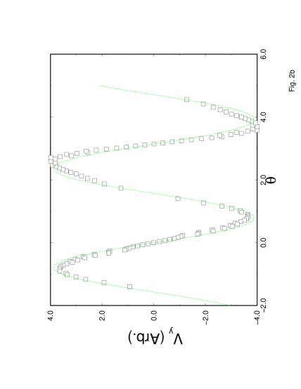
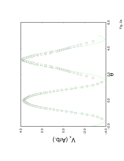
FIG. 2.:

REFERENCES

- [1] See, e.g., J. S. Langer, in Chance and Matter Les Houches Summer School (eds. J. Souletie, J. Vannimenus and R. Stora, North Holland, N.Y., 1086); Dynamics of Curved Fronts ( ed. R. Pelce, Academic, N.Y., 1988); D. Kessler, J. Koplik and H. Levine, Adv. Phys. 37, 255 (1988); J. S. Langer and L. Turski, Acta Metall. 25, 267 (1977); D. Jasnow and J. Viñals, Phys. Rev. 40, 3864 (1989).
- [2] K. Kawasaki and T. Ohta, Prog. Theor. Phys. 68 129 (1982); Physica A 118, 175 (1983).
- [3] H. Lamb, Hydrodynamics, sixth ed. (Dover, N. Y., 1932) Sec. 337.
- [4] N. O. Young, J. S. Goldstein, and M. J. Block, J. Fluid. Mech., 6, 350-356 (1959).
- [5] See, for example, the review article by R. S. Subramanian, in Transport Processes in Bubbles, Drops and Particles, ed. by R. P. Chhabra and D. De Kee, (Hemisphere Pub. Corp., N. Y. 1992).
- [6] R. Bhagavatula and D. Jasnow, J. Chem. Phys, July 1996.
- [7] P. C. Hohenberg and B. I. Halperin, Rev. Mod. Phys., 49, 435 (1977).
- [8] D. Jasnow and J. Vinals, Phys. of Fluids, 7, 747 (1996).
- [9] See eg., J. S. Langer, in Solids far from Equilibrium, ed. by C. Godreche (Cambridge 1992).
- [10] D. Jasnow, Rep. Prog. Phys. 47, 1059-1132 (1984).
- [11] S. Fisk and B. Widom, J. Chem. Phys. 50, 3219 (1969).
- [12] J. R. Rowlinson and B. Widom, Molecular Theory of Capillarity, (Clarendon Press, Oxford 1982).
- [13] For a recent review see, A. J. Bray, Adv. in Physics, 1996.
- [14] T. Ohta, Ann. Phys. (N.Y.) 158, 31(1984).
- [15] K. Kitahara, Y. Oono and D. Jasnow, Mod. Phys. Lett. B 2, 765 (1988).
- [16] J. Llambías and D. Jasnow (unpublished). Also, see J. Llambías, A. Shinozaki and D. Jasnow, NASA Conference Publication 3276, 207 (1994).
- [17] H. W. Alt and I. Pawlow, Physica D, 59, 389-416, (1992).
- [18] D. Boyanovsky, D. Jasnow, J. Llambías and F. Takakura, Phys. Rev. E 51, 5453 (1995).
- [19] R. Bhagavatula, J. Llambías and D. Jasnow, unpublished.
- [20] C. Yeung, J. M. Mozos, A. Hernandez-Machado and D. Jasnow, J. Stat. Phys. 70, 1149 (1993).
- [21] D. Jasnow and J. Viñals, Phys. Rev. A 41 6910 (1990).
- [22] S. Sarkar and D. Jasnow, Phys. Rev. A, 39, 5299 (1989). A numerical method of solving 2d interface equations of this sort is discussed, for example, by J. Vinals and D. Jasnow, Phys. Rev. A, 46, 7777 (1992).
- [23] G. Caginalp, Ann. Phys. (N.Y.) 172 136 (1986).
- [24] If the droplet were moving steadily as a solid object, the interface velocity would vanish in the CM frame, i.e., , the rest frame of the droplet. Then would have and .