Dimensional Crossover of Weak Localization in a Magnetic Field

Abstract

We study the dimensional crossover of weak localization in strongly anisotropic systems. This crossover from three-dimensional behavior to an effective lower dimensional system is triggered by increasing temperature if the phase coherence length gets shorter than the lattice spacing $a$. A similar effect occurs in a magnetic field if the magnetic length $L_{m}$ becomes shorter than $a(D_{\|}/D_{\perp})^{\gamma}$, where $D_{\|}/D_{\perp}$ is the ratio of the diffusion coefficients parallel and perpendicular to the planes or chains. $\gamma$ depends on the direction of the magnetic field, e.g. $\gamma=1/4$ or $1/2$ for a magnetic field parallel or perpendicular to the planes in a quasi two-dimensional system. We show that even in the limit of large magnetic field, weak localization is not fully suppressed in a lattice system. Experimental implications are discussed in detail.

]

I Introduction

Strongly anisotropic systems show a number of interesting and unusual physical properties. Many of these are due to the interplay of their lower dimensional substructures and three-dimensional coherence. Prominent examples are high $T_{c}$-superconductors in quasi two- and Peierls’ transitions in quasi one-dimensional systems. Also, weak localization (WL) – the subject of this paper – qualitatively and quantitatively depends on the effective dimension of the system.

It is important to distinguish two classes of anisotropic systems. The first class shares more or less the properties of typical three-dimensional systems, e.g. the Fermi surface is strongly anisotropic but closed, and the transport properties in different directions may vary by a large amount but still show a typical three-dimensional behavior.

More interesting is the second class where the distance of the planes or chains $a$ becomes an important new length scale. As far as electronic properties are concerned, we expect this to happen only for systems with an open Fermi surface. The distance $a$ should be compared with other characteristic length scales of the system, e.g. the phase-coherence length $L_{\varphi}$. In the regime of low temperatures $L_{\varphi}$ is large, $L_{\varphi}\gg a$, and even quasi one- or two-dimensional systems show three-dimensional behavior.

With increasing temperature or as a function of some external parameter like pressure or magnetic field, a dimensional crossover to one- or two-dimensional behavior can be observed, when $L_{\varphi}$ or an other relevant length scale gets to be smaller than the distance $a$ of the chains or planes.

An example for this phenomenon are certain disordered quasi one- or two-dimensional materials, which stay metallic at lowest temperatures, despite the fact that all one or two-dimensional disordered systems are insulators.

In this paper we will study the dimensional crossover of WL in strongly anisotropic $3D$ systems as a function of temperature (or phase-coherence time) and magnetic field [1]. We will argue that the magnetoresistance is an especially well suited tool to analyze the dimensional crossover. We will first concentrate on quasi two-dimensional systems of weakly coupled planes. The transverse and parallel conductivity is investigated in a magnetic field either parallel or perpendicular to the planes. We will also mention related results for quasi one-dimensional structures. At the end we will discuss experimental implications and the question of universality.

This work was motivated by recent experimental results on the quasi one-dimensional organic conductors $H_{2}(pc)I$ and $Ni(pc)I$, where “$pc$” stands for “phthalocyanine”, which appear to show a dimensional crossover in their WL correction to the conductivity [2].

II Weak Localization and Dimensional Crossover

WL [3, 4, 5] is a quantum-interference effect of (particle-) waves in a random medium. Consider the probability for a particle to return to the position where it has started[6]. For a quantum particle this probability is given by the modulus squared of the sum of transition amplitudes over all paths. Due to the random nature of the phases typically all interference effects vanish, resulting in a probability being that of a classical diffusion process. The cancelation of interference terms does not hold for time reversed paths, where the particle moves the same path clockwise and anti-clockwise, collecting the same phase. Thus this interference is constructive, therefore increasing the probability to return to the origin. As a consequence the diffusion constant and the conductivity decrease. In one or two dimensions, this so called “coherent back-scattering” finally leads to localization [1, 7]. As a magnetic field breaks the time-reversal invariance, leading to different Aharonov-Bohm phases for time-reversed paths, it destroys WL for all paths which include of the order of one or more flux-quanta [1].

Technically this process can be described by the contribution of maximally crossed diagrams to the conductivity [1, 3, 4]. In the hydrodynamic limit (${\bf q}\to 0,\omega\to 0$) these contributions sum up to a typical pole-structure, called cooperon, which (by time reversal) is directly related to the diffusion pole [7]. The cooperon $C({\bf r},t)$ is the solution of a diffusion equation [5]

$$\left[\partial_{t}+\sum_{\alpha}D_{\alpha\alpha}\hat{{\rm Q}}_{\alpha}^{2}+\frac{1}{\tau_{\varphi}}\right]C({\bf r},t)=\frac{1}{\tau_{\rm el}}\delta(t)\delta({\bf r}),$$ (1)

where we choose our coordinate system, so that the tensor of diffusion coefficients $D_{\alpha\beta}$ is diagonal.

$$\hat{{\rm{\bf Q}}}=-i\hbar{\bf\nabla}-(2e/c)\hat{{\rm{\bf A}}}$$ (2)

is the canonical momentum operator. We include the vector potential ${\bf A}$ throughout the paper in the definition of $\hat{{\rm{\bf Q}}}$ via minimal coupling in a semi-classical approximation. Note the factor of two in front of the charge, as the cooperon describes a two-particle process. The fact, that the particle looses its phase coherence due to electron-electron or electron-phonon interaction is described by the phase coherence time $\tau_{\varphi}$, which acts as an infrared-cutoff for (1). Only processes on time-scales shorter than $\tau_{\varphi}$ contribute to WL. Generally $\tau_{\varphi}$ and the elastic scattering time $\tau_{\rm el}$ will be ${\bf k}$-dependent especially in the strongly anisotropic systems we want to describe. However, we will neglect this for simplicity, as it should not affect our qualitative conclusions.

The correction $\Delta\sigma$ due to the cooperon to the Boltzmann conductivity $\sigma_{0,\alpha\beta}$ is given by

$$\Delta\sigma_{\alpha\beta} = e^{2}\int\frac{d{\bf k}}{(2\pi)^{3}}\int\frac{d{\bf Q}}{(2\pi)^{3}}$$ (4)

$$\raisebox{1.29167pt}{$\,\times\,$}v_{\alpha}({\bf k})|G_{{\bf k}}|^{2}C({\bf Q},\omega)|G_{{\bf Q}-{\bf k}}|^{2}v_{\beta}({\bf Q}-{\bf k});$$

${\bf v}({\bf k})=\partial_{{\bf k}}\epsilon_{{\bf k}}$ is the velocity. The Green’s functions $G_{{\bf k}}$ are sharply peaked in a region $\cal F$ of width $1/\tau_{\rm el}$ around the Fermi surface ($1/\tau_{\rm el}<E_{\rm F}$). Therefore, the ${\bf k}$-summation can be replaced by an average over the region $\cal F$, which we denote by $\left\langle\dots\right\rangle_{{\bf k}}$ and

$$\Delta\sigma_{\alpha\beta}=\frac{e^{2}\tau_{\rm el}^{2}}{\pi}\int\frac{d{\bf Q}}{(2\pi)^{3}}\left\langle v_{\alpha}({\bf k})v_{\beta}({\bf Q-k})\right\rangle_{{\bf k}}C({\bf Q},\omega).$$ (5)

To discuss the influence of a magnetic field it is essential to incorporate the vector potential in a gauge-invariant way. We therefore rewrite (5) in the manifestly gauge-invariant form

$$\Delta\sigma_{\alpha\beta}=\frac{e^{2}\tau_{\rm el}^{2}}{\pi V}{\rm Tr}\,\!\left[\left\langle\hat{{\rm v}}_{\beta}({\bf Q-k})\hat{{\rm v}}_{\alpha}({\bf k})\right\rangle_{{\bf k}}\hat{{\rm C}}({\bf Q},\omega)\right]_{{\bf Q}},$$ (6)

where the averaged velocities and the cooperon are understood as operators (we denote operators with a hat) in the center-of-mass space spanned by $\hat{{\bf Q}}$ or its conjugate position operator $\hat{{\bf r}}$. $V$ is the volume of the system.

When the average of the velocities is ${\bf Q}$ independent, as it is e.g. in an isotropic $3D$ system, using $\sigma_{0,\alpha\beta}(\omega=0,B=0)=e^{2}\left\langle v_{\alpha}v_{\beta}\right\rangle_{{\bf k}}=N_{0}e^{2}D_{\alpha\beta}$ for the static Boltzmann conductivity, formula (5) reduces to the well known form

$$\frac{\Delta\sigma}{\sigma_{0}}=-\frac{\tau_{\rm el}}{\pi N_{0}}C({\bf r}=0,\omega=0),$$ (7)

$N_{0}$ is the density of states at the Fermi-surface.

For the discussion of a dimensional crossover, it is essential to incorporate the spatial structure and the anisotropy of the system in the diffusion equation for the cooperon (1). The range of validity of the diffusion equation (1) for small distances is on the one hand restricted by the elastic scattering length $\l_{\alpha}=\sqrt{D_{\alpha\alpha}\tau_{\rm el}}$, on the other by the structure of the material, i.e. by the spacing $a$ of the planes in the anisotropic quasi $2D$ system. Therefore one has to distinguish the two scenarios mentioned in the introduction: in the first scenario, the elastic scattering length perpendicular to the planes $l_{\perp}$ is larger than the distance $a$ of the planes. Then the ultraviolet cutoff in the $q_{\perp}$-integration is given by $l_{\perp}^{-1}$ and the anisotropy of the diffusion-constant in (1) can be scaled out as previously shown [8]. Such a material will always show $3D$ behavior, as far as WL is concerned. We expect this first scenario, e.g. in all materials with a closed Fermi-surface, which can continuously be deformed to a sphere. The electronic properties of such systems are qualitatively not directly influenced by their lower dimensional substructures.

The second scenario is the more interesting one. Here $l_{\perp}$ is formally smaller than $a$ and the cutoff is now given by the substructure of the system, i.e. the distance of the planes. As we will see, these systems show a dimensional crossover and are affected by the underlying lattice structure. We expect this scenario to hold for anisotropic systems with an open Fermi-surface and quite strong short-range disorder.

We measure the anisotropy with the dimensionless constant

$$\eta=\frac{D_{\perp}\tau_{\rm el}}{a^{2}}=\left(\frac{l_{\perp}}{a}\right)^{2}.$$ (8)

For $\eta\ll 1$ we are in the second regime. In terms of microscopic quantities the diffusion constants are given by $D_{\perp}=t_{\perp}^{2}a^{2}\tau_{\rm el}/2$ or $\eta=(t_{\perp}\tau_{\rm el})^{2}/2$ for an effective hopping rate $t_{\perp}$ perpendicular to the planes. The diffusion constant for the motion in the planes is $D_{\|}=v_{\rm F}l/2$ where $l=v_{\rm F}\tau_{\rm el}$ is the (elastic) mean free path and $v_{\rm F}$ the Fermi velocity. A dimensional crossover should therefore be observable if the broadening due to elastic scattering is larger than the bandwidth $t_{\perp}$ perpendicular to the planes.

As it turns out, in the case of a finite magnetic field it is important to include the cutoffs of the cooperon-equation (1) in a gauge-invariant way. Therefore we will analyze the following cooperon-equation, here given for a quasi-$2D$ material with the symmetry axis in the $z$-direction and frequency $\omega=0$:

$$\left[D_{\|}\left(\hat{{\rm Q}}_{x}^{2}+\hat{{\rm Q}}_{y}^{2}\right)+\frac{4D_{\perp}}{a^{2}}\sin^{2}\frac{a\hat{{\rm Q}}_{z}}{2}+\frac{1}{\tau_{\varphi}}\right]C({\bf r})=\frac{1}{\tau_{\rm el}}\delta({\bf r}).$$ (9)

Eq. (9) is obtained from the result of summing the maximally crossed diagrams in zero magnetic field for a tight-binding model description of weakly coupled planes [9, 10, 11] by substituting the canonical momentum operator (2) for the Cooperon momentum $\hat{{\rm{\bf Q}}}$ in a quasi-classical approximation.

The ”bandstructure” $2\sin^{2}(aQ_{z}/2)=1-\cos aQ_{z}$ serves as a convenient physical way to introduce the cutoff $a$. Note that the details of the cutoff structure, i.e. the special form of the electronic bandstructure, will not affect any of our results qualitatively. In the $z$-direction the diffusion described by Eq. (9) takes place on a lattice with spacing $a$. For convenience we choose a gauge with $A_{z}=0$ in (9), otherwise the usual Peierls’ phase factors for a magnetic field on a lattice have to be introduced.

Dupuis and Montambaux [11] investigated the validity of the diffusion approximation for large magnetic fields analyzing the exact integral kernel for the cooperon. They concluded that (9) is valid for not too strong magnetic field $\omega_{c}\tau_{\rm el}\ll 1$. The cyclotron-frequency $\omega_{c}$ is given by $\omega_{c}=eB/mc$ for a magnetic field parallel to the planes (closed orbits) and by $\omega_{c}\approx eBv_{\rm F}a/c$ in the case of a magnetic field perpendicular to the planes (open orbits). A diffusion equation for the cooperon similar to (9) was analyzed by Nakhmedov et al.[10] to study the dimensional crossover from $d=1$ to $d=2$ two-dimensional system. Dorin [12] investigated quasi two-dimensional systems but considered only a magnetic field perpendicular to the planes. Dupuis and Montambaux [11] studied the conductivity in a strongly anisotropic two-dimensional system, but also for anisotropic three-dimensional materials. They focused their attention to the in-plane conductivity (see also Ref. [13]). We will argue below that for an experimental analysis of the effects of weak localization in a magnetic field, the comparison of in-plane and out-of-plane conductivity for both a magnetic field parallel and perpendicular to the planes is necessary. We will therefore discuss all four situations in detail for both small and large magnetic fields in the whole regime where (9) is valid.

III Quasi Two-Dimensional Systems

A Perpendicular Field

We first consider the effect of a magnetic field perpendicular to the planes of a quasi two-dimensional system. To model the system we assume an open Fermi-surface with a band-structure of the type $\epsilon_{{\bf k}}=(k_{x}^{2}+k_{y}^{2})/(2m)-2t_{\perp}\cos(ak_{z})$ with $t_{\perp}<1/\tau_{\rm el}<E_{\rm F}$. The details of $\epsilon_{{\bf k}}$ do not affect any of our qualitative results as long as the topology of the Fermi-surface remains unchanged.

For a magnetic field perpendicular to the planes the magnetic field only affects the motion in the planes. This situation was recently analyzed by Dorin [12]. In this section we will more or less rederive his results and establish notations and techniques for the more involved discussion of a magnetic field parallel to the planes.

1 Current in the planes

For the case of a current directed parallel to the planes the velocity average over the region $\cal F$ is given by

$$\left\langle v_{\|}({\bf k})v_{\|}({\bf Q-k})\right\rangle_{{\bf k}}=-\frac{1}{2}v_{\rm F}^{2}.$$ (10)

To calculate the WL correction to the in-plane conductivity $\Delta\sigma_{{\bf B}\|\hat{{\bf z}}}^{\|}$, the trace in (6) is expanded in normalized eigenfunctions $\Phi_{\lambda}$ of the operator on the left-hand side of (9) for $\omega=0$ defined by

$$\left[D_{\|}\left({Q}_{x}^{2}+{Q}_{y}^{2}\right)+\frac{4D_{\perp}}{a^{2}}\sin^{2}\frac{a{Q}_{z}}{2}+\frac{1}{\tau_{\varphi}}\right]\Phi_{\lambda}=E_{\lambda}\Phi_{\lambda}.$$ (11)

As the velocity average is just a constant, $\Delta\sigma_{{\bf B}\|\hat{{\bf z}}}^{\|}$ can be expressed in terms of the eigenvalues $E_{\lambda}$

$$\frac{\sigma_{{\bf B}\|\hat{{\bf z}}}^{\|}}{\sigma_{0}}=-\frac{1}{\pi N_{0}V}\sum_{\lambda}\frac{1}{E_{\lambda}}$$ (12)

with $N_{0}\approx m/(2\pi a)$. The ultra-violet cutoff can be imposed in a gauge invariant way by requiring $E_{\lambda}\lesssim 1/\tau_{\rm el}$.

For the calculation we choose the gauge ${\bf A}_{\perp}=(0,Bx,0)$. The strength of the magnetic field is measured by the magnetic length $L_{m}=\sqrt{\hbar c/eB}$. The eigenfunctions $\Phi_{\lambda}$ can be decomposed in plane waves in the $y$- and $z$-direction carrying momenta $q_{y}$ and $q_{z}$ and a remaining part, which describes a shifted one-dimensional harmonic oscillator (HO) for a particle of “mass” $(2D_{\|})^{-1}$ and “cyclotron frequency” $\Omega_{\perp}=4D_{\|}eB/c=4D_{\|}/L_{m}^{2}$ with eigenfunctions $\Psi^{\rm HO}_{n}(x+L_{m}^{2}q_{y}/2)$ and eigenvalues $E^{\prime}_{n}=(n+1/2)\Omega_{\perp}$, $n=0,1,2,\dots$. Note that $\Omega_{\perp}$ is by a factor of $4D_{\|}m\approx 4E_{\rm F}\tau_{\rm el}$ larger than the cyclotron frequency of bare electrons. Therefore a weak magnetic field is sufficient to have a strong effect on WL.

The DC-conductivity is found from (12) as

$$\frac{\Delta\sigma_{{\bf B}\|\hat{{\bf z}}}^{\|}}{\sigma_{0}^{\|}}=\frac{-1}{L_{m}^{2}\pi^{2}N_{0}}\sum_{n,q_{z}}\left({E_{n}^{\prime}+\frac{4D_{\perp}}{a^{2}}\sin^{2}\frac{aq_{z}}{2}+\frac{1}{\tau_{\varphi}}}\right)^{-1}.$$ (13)

The factor $2/(2\pi L_{m}^{2})$ takes care of the degeneracy of the “Landau levels” of the cooperon with charge $2e$. For $\eta<1$, $q_{z}$ is integrated over the whole Brillouin zone $|q_{z}|<\pi/a$ leading to

$$\frac{\Delta\sigma_{{\bf B}\|\hat{{\bf z}}}^{\|}}{\sigma_{0}^{\|}}=-\lambda\sum_{\epsilon_{n}=(n+\frac{1}{2})w_{\perp}}\frac{w_{\perp}\,g_{c}(\epsilon_{n})}{\sqrt{\epsilon_{n}+x}\sqrt{\epsilon_{n}+x+4\eta}}.$$ (14)

Here we have introduced the dimensionless quantities

$$x=\frac{\tau_{\rm el}}{\tau_{\varphi}},\quad\lambda=(2\pi E_{\rm F}\tau)^{-1},\quad w_{\perp}=\Omega_{\perp}\tau_{\rm el}=\frac{4l_{\|}^{2}}{L_{m}^{2}}$$ (15)

to measure the rate of phase-destruction, the strength of disorder and the cyclotron frequency. Sometimes it is useful to interpret $w_{\perp}$ as the inverse area occupied by a flux quantum in units of a typical area, where elastic processes take place. $g_{c}(x)$ is a cutoff-function of scale unity — for our plots we use $g_{c}(x)=\exp(-\pi x^{2}/4)$ whereas our analytical formulas are given for the step function $g_{c}(x)=\Theta(1-x)$.

For weak magnetic field $w_{\perp}\to 0$, the sum (14) can be approximated by an integral, and the effects of discretization can be calculated using the Euler-Maclaurin summation formula. For the different regimes we find the following analytical approximations

$$\frac{\Delta\sigma_{{\bf B}\|\hat{{\bf z}}}^{\|}}{\sigma_{0}^{\|}} \approx -\lambda\left\{\begin{array}[]{l@{\quad}l}\alpha^{\|}-\beta_{{\bf B}\|\hat{{\bf z}}}^{\|}w_{\perp}^{2},&w_{\perp}\ll x,\eta\\ \displaystyle\alpha^{\|}-c\sqrt{{w_{\perp}}/{\eta}},&x\ll w_{\perp}\ll\eta\\ \displaystyle\gamma+\log({4}/{w_{\perp}}),&x,\eta\ll w_{\perp}\ll 1\\ 2g_{c}(w_{\perp}/2),&w_{\perp}\gg 1\\ \propto 1/x,&x\gg 1\end{array}\right.$$ (21)

with Euler’s Gamma constant $\gamma$, a constant $c=(\zeta(1/2)/2)(1-\sqrt{2})\approx 0.3024$ and

$$\alpha^{\|}(\eta,x) = \int_{0}^{\infty}\frac{g_{c}(\epsilon)}{\sqrt{\epsilon+x}\sqrt{\epsilon+x+4\eta}}\,d\epsilon$$ (22)

$$= \kappa_{1}(x+1)-\kappa_{1}(x)$$ (23)

$$\beta_{{\bf B}\|\hat{{\bf z}}}^{\|}(\eta,x) = -(2\eta+z)\lambda_{1}(z)\Big{|}_{z=x}^{x+1}\approx(2\eta+x)\lambda_{1}(x).$$ (24)

We have introduced for later convenience the functions $\kappa_{1},\lambda_{1}$

$$\kappa_{1}(z) = 2\log\left(\sqrt{z}+\sqrt{z+4\eta}\right)$$ (25)

$$\lambda_{1}(z) = \frac{1}{24z^{3/2}(z+4\eta)^{3/2}}.$$ (26)

A graphical representation based on a numerical evaluation of (14) is given in Fig. 1.

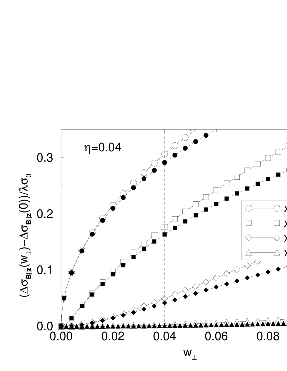
FIG. 1.: The magneto-conductivity for a field perpendicular to the planes as a function of magnetic field $w_{\perp}=4l_{\|}^{2}/L_{m}^{2}$ for various temperatures, i.e. various phase coherence times $x=\tau_{\rm el}/\tau_{\varphi}$. The open and filled symbols denote the conductivity parallel and perpendicular to the planes, respectively. The crossover scale $w_{\perp}=\eta=0.04$ is shown as a dashed line. The lines are guides to the eye.

In the limit $\eta\to 0$ one recovers the well known $2D$ results [1]. The precise form of $\alpha^{\|}(\eta,x)$ and the constant contribution in the regime $x,\eta\ll w_{\perp}\ll 1$ depend slightly on the cutoff structure, i.e. on $g_{c}$.

Using (23), we can now discuss the dimensional crossover as a function of temperature in the absence of a magnetic field. To a good approximation the only temperature dependent quantity in our model is the phase-coherence time contained in the parameter $x=\tau_{\rm el}/\tau_{\varphi}$. Usually its temperature dependence can be approximated by a power law $x\propto T^{\gamma}$, where $\gamma$ depends on the dominant scattering process [1, 14].

For $x<\eta$, i.e. if the phase-coherence length $\sqrt{D_{\perp}\tau_{\varphi}}$ is larger than the distance of the planes $a$, the usual three-dimensional behavior is observed. For not too strong disorder the system is metallic as the correction due to WL is finite for $T\to 0$, i.e. $x\to 0$. The leading temperature dependence is given by the contribution proportional to $\sqrt{x/\eta}$ – again typical for WL in a $3D$ system. However, at higher temperatures the coherence between the planes is destroyed and the behavior of the system is dominated by the two-dimensional planes. As a consequence, we obtain the logarithmic correction $\Delta\sigma/\sigma_{0}\approx-\lambda\log x$ typical for WL in two dimensions.

The magneto-conductivity at low temperature rises quadratically with the magnetic field for $w_{\perp}\ll x$, i.e. as long as a particle can not enclose a flux quantum in a coherent diffusion process. For a higher field, the magneto-conductivity (cf. Fig. 1) increases with the square-root of the magnetic field in the three-dimensional regime with $x\ll w_{\perp}\ll\eta$. Note that corrections to the square-root dependence are of the order of $x/\sqrt{w_{\perp}\eta}$, therefore this regime can only be observed at quite low temperatures. By increasing the magnetic field even more, the WL corrections crosses over to a logarithmic dependence on field. Finally, at a very high field when $w_{\perp}\gg 1$, WL is destroyed completely (not shown in Fig. 1).

2 Current perpendicular to the planes

For the case of the current perpendicular to the planes, the velocity average is now ${\bf Q}$ dependent

$$\left\langle v_{\perp}({\bf k})v_{\perp}({\bf Q-k})\right\rangle_{{\bf k}} \approx -\frac{1}{2}t_{\perp}^{2}a^{2}\cos(aQ_{\perp})$$ (27)

$$= -\frac{D_{\perp}}{\tau_{\rm el}}\cos(aQ_{\perp}).$$ (28)

While (28) depends on the details of the band-structure, our results are nearly independent of these details. Our conclusions rely on the generic feature that $\left\langle v_{\perp}({\bf k})v_{\perp}({\bf Q-k})\right\rangle_{{\bf k}}\to const.$ for $Q_{\perp}\to 0$ and on $\int dQ_{\perp}\left\langle v_{\perp}({\bf k})v_{\perp}({\bf Q-k})\right\rangle_{{\bf k}}=0$. The last fact is a consequence of the periodicity of $\epsilon_{{\bf k}}$.

In the chosen gauge ($A_{\perp}=(0,0,By)$), $Q_{\perp}=q_{z}$ is a good quantum number. Therefore it is easy to add the factor $\cos aq_{z}$ in (13) and the WL correction perpendicular to the planes has the form[12]

$$\frac{\Delta\sigma_{{\bf B}\|\hat{{\bf z}}}^{\perp}}{\sigma_{0}^{\perp}} = -\frac{\lambda}{4\eta}\sum_{\epsilon_{n}=(n+\frac{1}{2})w_{\perp}}\frac{w_{\perp}\,g_{c}(\epsilon_{n})}{\sqrt{\epsilon_{n}+x}\sqrt{\epsilon_{n}+x+4\eta}}$$ (30)

$$\qquad\raisebox{1.29167pt}{$\,\times\,$}\left(\sqrt{\epsilon_{n}+x+4\eta}-\sqrt{\epsilon_{n}+x}\right)^{2}.$$

Again, analytical approximations can be found in the different regimes:

$$\frac{\Delta\sigma_{{\bf B}\|\hat{{\bf z}}}^{\perp}}{\sigma_{0}^{\perp}} \approx -\lambda\left\{\begin{array}[]{l@{\quad}l}\alpha^{\perp}-\beta_{{\bf B}\|\hat{{\bf z}}}^{\perp}w_{\perp}^{2},&w_{\perp}\ll x,\eta\\ \alpha^{\perp}-c\sqrt{{w_{\perp}}/{\eta}},&x\ll w_{\perp}\ll\eta\\ {(\eta\pi^{2})}/{(2w_{\perp})},&x,\eta\ll w_{\perp}\ll 1\\ \frac{4\eta}{w_{\perp}}g_{c}\left({w_{\perp}}/{2}\right),&w_{\perp}\gg 1\\ \propto 1/x^{2},&x\gg 1\end{array}\right.$$ (36)

with the numerical constant $c\approx 0.30$ as before,

$$\alpha^{\perp}(\eta,x) = \frac{1}{2\eta}\left(\sqrt{z(z+4\eta)}-z\right)\Big{|}_{z=x}^{1+x}$$ (37)

$$\beta_{{\bf B}\|\hat{{\bf z}}}^{\perp}(\eta,x) = -2\eta\lambda_{1}(z)\Big{|}_{z=x}^{x+1}\approx 2\eta\lambda_{1}(x).$$ (38)

$\lambda_{1}$ is defined by Eq. (26).

For small fields and low temperatures $w_{\perp},x\ll\eta$, the main contribution is due to the Cooper-pole with ${\bf Q}\approx 0$ and therefore $\cos aq_{z}\approx 1$. As a consequence we get practically the same answers for both directions of the current as can be seen in Fig. 1. However, at high fields $w_{\perp}\gg\eta$ (not shown in Fig. 1, see Fig. 3) or temperatures $x\gg\eta$ the WL correction $\Delta\sigma_{{\bf B}\|\hat{{\bf z}}}^{\perp}$ vanishes faster because the coherence among different planes is destroyed. A crossover from three- to zero-dimensional behavior is observed [12].

B Parallel Field

1 Current in the planes

More interesting is a magnetic field parallel to the planes. We will first discuss the case of a current in the planes where the average of the velocities is given by (10). We choose the gauge ${\bf A}_{\|}=(0,-Bz,0)$ for a magnetic field in $x$-direction. Again, the eigenfunctions defined in (11) can be decomposed in plane waves in $x$ and $y$ direction with momenta $q_{x}$ and $q_{y}$ and a non trivial part. Therefore we have to analyze the remaining “Hamiltonian”:

$$\hat{{\rm H}}^{\prime}=D_{\|}\left(\hat{{\rm q}}_{y}+\frac{2\hat{{\rm z}}}{L_{m}^{2}}\right)^{2}+\frac{2D_{\perp}}{a^{2}}\left(1-\cos a\hat{{\rm q}}_{z}\right).$$ (39)

This is the Hamiltonian of a one-dimensional tight-binding lattice with hopping-rate $D_{\perp}/a^{2}$ and an external harmonic potential, centered at $-q_{y}L_{m}^{2}/2$, with oscillator frequency $\Omega_{\|}=4\sqrt{D_{\perp}D_{\|}}/L_{m}^{2}=\Omega_{\perp}\sqrt{D_{\perp}/D_{\|}}$. The corresponding “Schrödinger equation” can be identified with Mathieu’s equation [15, 10].

For low quantum numbers and low energies, only the quadratic part of the kinetic energy of $H^{\prime}$ is probed, therefore the wave-functions have approximately HO from as above. Their energy is given by $E_{n}^{\prime}\approx\Omega_{\|}(n+1/2)$. This contribution will dominate for a weak magnetic field. We can estimate the range of validity from the condition $q_{z}\lesssim 1/a$ using a characteristic momentum $q_{z,typ}\approx\sqrt{2mn\Omega_{\|}}$ and get $n\lesssim n_{c}=c^{\prime}\eta/w_{\|}$, where $c^{\prime}$ is a constant of order one. A comparison with numerical results suggests the value $c^{\prime}\approx 2$. We have introduced as above the dimensionless constant $w_{\|}=\Omega_{\|}\tau_{\rm el}=4l_{\perp}l_{\|}/L_{m}^{2}$. In Fig. 2 we compare the numerically calculated spectrum of $H^{\prime}$ with this analytical approximation. The contribution of these lowest eigenvalues is approximately given by

$$\displaystyle\left(\frac{\Delta\sigma_{{\bf B}\perp\hat{{\bf z}}}^{\|}}{\sigma_{0}^{\|}}\right)_{\rm HO}=-\lambda K_{1}$$ (40)

$$\displaystyle K_{1}=\frac{w_{\|}}{\pi\sqrt{\eta}}\sum_{n=0}^{\infty}\frac{g_{c}\left[\left(n+\frac{1}{2}\right)\frac{w_{\|}}{2\eta}\right]\arctan\left(\epsilon_{n}+x\right)^{-1/2}}{\sqrt{\epsilon_{n}+x}}.$$ (41)

Note the factor $2\eta$ in the cutoff-function taking into account the condition $n<n_{c}$. The energies are given by $\epsilon_{n}=(n+1/2)w_{\|}$. Actually it turns out that for $w_{\|}\approx\eta$, i.e. in the crossover region, the main contribution to the magneto-conductivity is due to the lowest eigenstate $\epsilon_{0}$. In the same region the approximation $\epsilon_{0}\approx w_{\|}/2$ breaks down. Therefore we use for our numerical evaluations of (41) a more accurate expression for the ground-state energy

$$\epsilon_{0}=2\eta\frac{8u^{4}+7u^{2}+16u}{8u^{4}+15u^{3}+16u+32},\qquad u=\frac{w_{\|}}{2\eta}.$$ (42)

This interpolating formula describes the ground state energy of (39) exactly in next-to-leading order[15] in both $w_{\|}/\eta$ and $\eta/w_{\|}$. Especially, for $w_{\|}\to 0$ it reduces to $\epsilon_{0}\approx w_{\|}/2$ and for large magnetic field to $\epsilon_{0}\approx 2\eta$.

For high quantum numbers $n\gtrsim n_{c}$, the potential energy dominates and the hopping rate is small compared to the level-splitting due to the external potential. In this regime the eigenfunctions are localized in one plane and we can approximate

$$\hat{{\rm H}}^{\prime}\approx D_{\|}\left(\hat{{\rm q}}_{y}+\frac{2\hat{{\rm z}}}{L_{m}^{2}}\right)^{2}+\frac{2D_{\perp}}{a^{2}}.$$ (43)

$\hat{{\rm z}}$ denotes the position of the planes and has the eigenvalues $na$, $n=0,\pm 1,\dots$. Therefore the higher eigenvalues of $\hat{{\rm H}}^{\prime}$ are approximately given by

$$E^{\prime}_{n}\approx D_{\|}\left(q_{y}+\frac{2}{L_{m}^{2}}na\right)^{2}+\frac{2D_{\perp}}{a^{2}}.$$ (44)

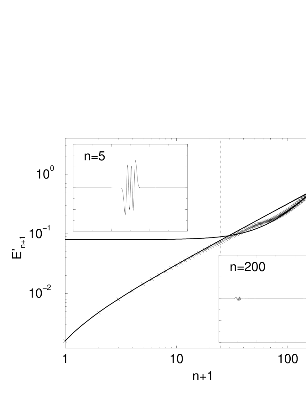
FIG. 2.: Numerically calculated spectrum (crosses) of the “Hamiltonian” (39) with $q_{y}=0$ for a lattice with $300$ sites in a log-log plot. For small quantum numbers, the dispersion is linear, whereas for high quantum numbers, it crosses over to a quadratic dependence. The solid lines represents our approximations $\epsilon_{n}=(n+1/2)w_{\|}$ or $\epsilon_{n}=2\eta+(n/2)^{2}w_{\|}^{2}/(4\eta)$, respectively. For the plot we have chosen $2\eta=0.04$ and $w_{\|}=0.0032$. In the insets, we show typical eigenfunctions in both regimes. The crossover scale $n_{c}=2\eta/w_{\|}$ is shown as a dashed line.

That this approximation is very accurate, is shown in Fig. 2 where we compare our approximation to a numerically determined spectrum of $\hat{{\rm H}}^{\prime}$. As the crossover regime will depend in any case on the (often unknown) details of band-structure and scattering rates and will influence our results not qualitatively, we will just sum up the contributions from the two regimes with the proper cutoff, denoted by the dashed line in Fig. 2.

Thus from (12) we get the following contribution from the second regime:

$$\left(\frac{\Delta\sigma_{{\bf B}\perp\hat{{\bf z}}}^{\|}}{\sigma_{0}^{\|}}\right)_{\rm loc}=-\lambda(K_{2}-K_{3})$$ (45)

with

$$K_{2} = \int_{0}^{\infty}\frac{g_{c}(q^{2})}{q^{2}+2\eta+x}dq^{2}\approx\log\frac{2\eta+x+1}{2\eta+x}$$ (46)

$$K_{3} = \frac{w_{\|}}{\pi\sqrt{\eta}}\sum_{n=0}^{\infty}\frac{g_{c}\left[\left(n+\frac{1}{2}\right)\frac{w_{\|}}{2\eta}\right]\arctan\left(2\eta+x\right)^{-1/2}}{\sqrt{2\eta+x}}$$ (47)

$$\approx \frac{1}{\sqrt{4\eta(2\eta+x)}}\raisebox{1.29167pt}{$\,\times\,$}\left\{\begin{array}[]{l@{\quad}l}2\eta,&w_{\|}\ll\eta\\ \displaystyle w_{\|}g_{c}\left(\frac{w_{\|}}{4\eta}\right),&w_{\|}\gg\eta\end{array}\right..$$ (50)

$K_{2}$ is the contribution one obtains from a summation over all  eigenvalues of (43). It is independent of the magnetic field. As (43) does describes only the eigenstates of (39) for $n>n_{c}=2\eta/w_{\|}$, we have to subtract the first $n_{c}$ eigenvalues summing up to $K_{3}$.

A direct interpretation of (46) can be given: As long as the particle moves in the plane, no flux is enclosed as the magnetic field is parallel to the motion. Therefore we find a contribution independent of the magnetic field. For $\eta=0$, i.e. in the true $2D$ situation, we recover the usual two-dimensional result as $K_{2}=\alpha^{\|}(\eta=0,x)=\log(1+1/x)$ and $K_{1}=K_{3}=0$. However, for a finite diffusion rate perpendicular to the planes there is an infrared cutoff due to the fact that the particle eventually leaves the particular plane it has been moving in. $K_{2}$ is exactly the formula describing WL in a two-dimensional system, however $1/\tau_{\varphi}$ is replaced by $1/\tau_{\varphi}+2/\tau_{a}$, where $\tau_{a}=\tau_{\rm el}/\eta=a^{2}/D_{\perp}$ is the time needed to diffuse to a neighboring plane. As a result, for very low temperatures $K_{2}$ saturates at $K_{2}(x=0)\approx\log 1/\eta$, instead of diverging as for a $2D$ system.

To discuss the magnetoresistance for a finite magnetic field parallel to the planes we have to add the contribution from the HO- and the localized regime

$$\frac{\Delta\sigma_{{\bf B}\perp\hat{{\bf z}}}^{\|}}{\sigma_{0}^{\|}}\approx-\lambda(K_{1}+K_{2}-K_{3}).$$ (51)

An analytic evaluation yields the following expression in the various regimes

$$\frac{\Delta\sigma_{{\bf B}\perp\hat{{\bf z}}}^{\|}}{\sigma_{0}^{\|}}\approx-\lambda\left\{\begin{array}[]{l@{\quad}l}\alpha^{\|}-\beta_{{\bf B}\perp\hat{{\bf z}}}w_{\|}^{2},&w_{\|}\ll x,\eta\\ \alpha^{\|}-c\sqrt{{w_{\|}}/{\eta}},&x\ll w_{\|}\ll\eta\\ \displaystyle K_{2},&w_{\|}\gg\eta,x\\ \propto 1/x,&x\gg 1\end{array}\right.$$ (52)

with

$$\beta_{{\bf B}\perp\hat{{\bf z}}} = \lambda_{2}(x+2\eta)-\lambda_{2}(x)$$ (53)

$$\lambda_{2}(z) = -\frac{1}{48\pi\sqrt{\eta}}\left[z^{-3/2}\arctan\frac{1}{\sqrt{z}}+\frac{1}{z(1+z)}\right].$$ (54)

As in the case of a perpendicular field, the (negative) magnetoresistance rises quadratically with magnetic field for $w_{\|}\ll x,\eta$ and then crosses over to a square-root dependence on $B$ or $w_{\|}$.

In contrast to the usual three-dimensional situation or a magnetic field perpendicular to the planes, the WL correction for magnetic field parallel to the planes does not vanish in a large magnetic field. The contribution $K_{2}$ remains finite even at very high fields[10, 11] as explained above.

At very high fields, $\omega_{c}\tau\gg 1$ or $w_{\|}\gg\sqrt{\eta}$ the diffusion approximation (9) breaks down as has been investigated by Dupuis and Montambaux [11]. They find that for very high fields $w_{\|}\gg 1$ the wave function of the electrons is localized in the planes leading to a strong suppression of hopping to neighboring planes. As the motion in the planes is not affected by a parallel magnetic field the effect of weak localization increases for a stronger magnetic field in this regime. As a consequence a positive magnetoresistance is expected for theses extremely high fields.

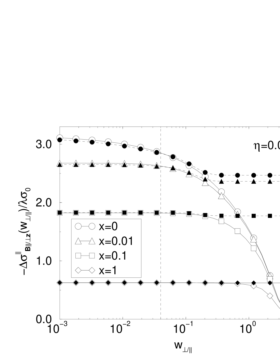
FIG. 3.: Comparison of the WL correction of the in-plane conductivity for a magnetic field parallel to a field perpendicular to the planes for various phase coherence times $x=\tau_{\rm el}/\tau_{\varphi}$, $\eta=0.04$. Note that on the $x$-axis different scales have been used: $w_{\|}=4l_{\perp}l_{\|}/L_{m}^{2}$ for a magnetic field in the planes (filled symbols) and $w_{\perp}=4l_{\|}^{2}/L_{m}^{2}=w_{\|}\sqrt{D_{\|}/D_{\perp}}$ for a magnetic field in the perpendicular direction (empty symbols). The crossover scale $w_{\perp/\|}\sim\eta$ is shown as a dashed line. The lines are guides to the eye.

In Fig. 3, the effects of a magnetic field parallel and perpendicular to the planes are compared. In the low temperature regime $x\ll\eta$, the dimensional crossover is induced by the magnetic field for $w_{\perp}\sim\eta$ (field perpendicular to the planes) or $w_{\|}\sim\eta$ (field parallel to the planes). For higher temperatures $x\gtrsim\eta$, such an crossover can not be observed because it is already preempted by the phase destroying scattering. At very high magnetic field $w_{\|}\gg\eta$, a finite contribution of WL remains when the field is parallel to the planes.

2 Current perpendicular to the planes

To calculate the out-of-plane WL-correction to the conductivity, we have to analyze (6) using the velocity average (28). Expanding the trace in (6) in eigenfunctions $\left|\Phi_{\lambda}\right\rangle$ of the cooperon defined in (11), we obtain

$$\frac{\Delta\sigma_{{\bf B}\perp\hat{{\bf z}}}^{\perp}}{\sigma_{0}^{\perp}}=-\frac{1}{\pi N_{0}V}\sum_{\lambda}\frac{\left\langle\Phi_{\lambda}\right|\cos a\hat{Q}_{z}\left|\Phi_{\lambda}\right\rangle}{E_{\lambda}}.$$ (55)

For the gauge ${\bf A}=(0,-Bz,0)$ we can interpret the cosine as a translation operator by one lattice site. In position space (note that we are considering a lattice in the $z$-direction) the overlap is therefore given by

$$\left\langle\Phi_{\lambda}\right|\cos a\hat{Q}_{z}\left|\Phi_{\lambda}\right\rangle = \sum_{n}\int dx\,dy$$ (57)

$$\raisebox{1.29167pt}{$\,\times\,$}{\,\rm Re}\left[\Phi^{*}_{\lambda}(x,y,an+a)\Phi_{\lambda}(x,y,an)\right].$$

where $n$ sums over the planes with distance $a$.

In the previous section we have shown that for low quantum numbers, the eigenfunctions $\left|\Phi_{\lambda}\right\rangle$ can be approximated by HO-eigenfunctions: $\Phi_{q_{x},q_{y},n}(x,y,z)\approx e^{iq_{x}x}\Psi_{n}^{\text{HO}}(z-L_{m}^{2}q_{y}/2)$. In this regime $a$ is small compared to the scale $\Delta_{n}$ on which $\Psi_{n}^{\text{HO}}(z)$ varies and $\left\langle\Phi_{\lambda}\right|\cos a\hat{Q}_{z}\left|\Phi_{\lambda}\right\rangle\approx 1+O((a/\Delta_{n})^{2})$. The scale $\Delta_{n}$ is of the order of half the distance of the nodes in $\Psi_{n}^{\text{HO}}(z)$, i.e. $\Delta_{n}\approx\sqrt{D_{\perp}/(n\Omega_{\|})}$.

For $a\gtrsim\Delta_{n}$ the overlap $\left\langle\Phi_{\lambda}\right|\cos a\hat{Q}_{z}\left|\Phi_{\lambda}\right\rangle$ vanishes on average. The condition for the crossover $a\approx\Delta_{n_{c}}$, i.e. $n_{c}\approx 2\eta/w_{\|}$ coincides with our previous estimate of the crossover to the localized regime which is described by (43). As the eigenfunctions of (43) are strictly localized on a single plane, it is consistent to approximate $\left\langle\Phi_{\lambda}\right|\cos a\hat{Q}_{z}\left|\Phi_{\lambda}\right\rangle=0$ for $n>n_{c}$.

Within these approximations the only contribution to (55) stems from the HO regime. This contribution has already been given in (41) and therefore

$$\frac{\Delta\sigma_{{\bf B}\perp\hat{{\bf z}}}^{\perp}}{\sigma_{0}^{\perp}} \approx -\lambda K_{1}$$ (58)

$$\approx -\lambda\left\{\begin{array}[]{l@{\quad}l}\alpha^{\perp}-\beta_{{\bf B}\perp\hat{{\bf z}}}w_{\|}^{2},&w_{\|}\ll x,\eta\\ \alpha^{\perp}-c\sqrt{{w_{\|}}/{\eta}},&x\ll w_{\|}\ll\eta\\ \sqrt{\frac{w_{\|}}{2\eta}}g_{c}\left(\frac{w_{\|}}{4\eta}\right),&\eta,x\ll w_{\|}\\ \propto 1/x,&x\gg 1\end{array}\right.$$ (63)

with

$$K_{1}(w_{\|}\to 0)\approx\kappa_{2}(x+2\eta)-\kappa_{2}(x)$$ (64)

$$\displaystyle\kappa_{2}(z)=\frac{1}{\pi\sqrt{\eta}}\left[2\sqrt{z}\arctan\frac{1}{\sqrt{z}}+\log{(1+z)}\right].$$ (65)

Note that $K_{1}(w_{\|}\to 0)$ does not coincide exactly with $\alpha^{\perp}$ given in (37), this is due to the approximation $\left\langle\Phi_{\lambda}\right|\cos a\hat{Q}_{z}\left|\Phi_{\lambda}\right\rangle\approx 1$ which slightly influences the contributions from higher energies (this explains the small offset in Fig. 3 for $w_{\|/\perp}\to 0$). The qualitative behavior, especially for low temperatures is however not affected.

As $K_{2}$ is independent and $K_{3}$ only a smooth function of the magnetic field, the magnetoresistance in a field parallel to the planes is more or less independent of the direction of the applied voltage. The main difference of $\Delta\sigma_{{\bf B}\perp\hat{{\bf z}}}^{\perp}/\sigma_{0}^{\perp}$ to $\Delta\sigma_{{\bf B}\perp\hat{{\bf z}}}^{\|}/\sigma_{0}^{\|}$ is the magnetic field independent, but temperature dependent contribution $K_{2}$.

Our analysis of (57) clearly indicates that the coherent transport between different planes is essential for the WL correction to the out-of-plane conductivity. This has e.g. the consequence that for a strong magnetic field parallel to the plane ($w_{\|}\gg\eta$) the WL correction to the out-of-plane conductivity is totally suppressed, while the conductivity parallel to the planes is still affected by interference effects of electrons moving in a plane.

IV Quasi One-Dimensional Systems

Now, we will briefly discuss the quasi $1D$-case, concentrating on a magnetic field perpendicular to the chains. We choose the symmetry axis in the $z$-direction so that the analog of (9) reads

$$\left[D_{\|}\hat{{\rm Q}}_{\|}^{2}+\frac{4D_{\perp}}{a^{2}}\sum_{i=x,y}\sin^{2}\frac{a\hat{{\rm Q}}_{i}}{2}+\frac{1}{\tau_{\varphi}}\right]C({\bf r})=\frac{1}{\tau_{\rm el}}\delta({\bf r}).$$ (66)

A straightforward calculation similar to the calculation for the quasi two-dimensional case with a magnetic field along the $x$-axis and vector potential $A_{\perp}=(0,0,By)$ yields (using the appropriate density of states $N_{0}^{1d}\approx(\pi v_{\rm F}a^{2})^{-1}$) the following quantum correction to the conductivity for a current parallel to the chains

$$\frac{\Delta\sigma_{{\bf B}\perp\hat{{\bf z}}}^{1d}}{\sigma_{0}}\approx-\frac{K_{1}^{1d}+K_{2}^{1d}-K_{3}^{1d}}{4\pi\sqrt{\eta}}$$ (67)

where $K_{1,2,3}^{1d}$ are given by

$$K_{1}^{1d} = \sum_{n=0}^{\infty}\frac{w_{\|}\,g_{c}\left[\left(n+\frac{1}{2}\right)\frac{w_{\|}}{2\eta}\right]}{\sqrt{\epsilon_{n}+x}\sqrt{\epsilon_{n}+x+4\eta}}$$ (68)

$$K_{2}^{1d} = 4\sqrt{\eta}\int_{0}^{\infty}\frac{g_{c}(q^{2})\,dq}{\sqrt{2\eta+x+q^{2}}\sqrt{6\eta+x+q^{2}}}$$ (69)

$$\approx \left\{\begin{array}[]{l@{\quad}l}\tilde{c}-4\sqrt{\eta},&x\ll\eta\\ 2\pi\sqrt{\eta/x}&\eta\ll x\ll 1\\ 4\sqrt{\eta}/x&x\gg 1\end{array}\right.$$ (73)

$$K_{3}^{1d} = \sum_{n=0}^{\infty}\frac{w_{\|}\,g_{c}\left[\left(n+\frac{1}{2}\right)\frac{w_{\|}}{2\eta}\right]}{\sqrt{x+2\eta}\sqrt{x+6\eta}}$$ (74)

with $\epsilon_{n}=(n+\frac{1}{2})w_{\|}$ and a numerical constant $\tilde{c}\approx 3.31$. Note, that for the numerical evaluation of (68), the lowest energy value $\epsilon_{0}$ should be treated special according to (42).

The limiting behavior of $\Delta\sigma$ in the various regimes is given by

$$\frac{\Delta\sigma_{{\bf B}\perp\hat{{\bf z}}}^{\|,1d}}{\sigma_{0}}\approx\frac{-1}{4\pi\sqrt{\eta}}\left\{\begin{array}[]{l@{\quad}l}\alpha^{\|}_{1d}-\beta_{{\bf B}\perp\hat{{\bf z}}}^{1d}w_{\|}^{2},&w_{\|}\ll x,\eta\\ \alpha^{\|}_{1d}-c\sqrt{{w_{\|}}/{\eta}},&x\ll w_{\|}\ll\eta\\ \displaystyle K_{2}^{1d},&\eta\ll w_{\|}\\ \propto 1/x,&x\gg 1\\ \end{array}\right.$$ (75)

with $c\approx 0.30$ and

$$\alpha^{\|}_{1d} \approx \frac{2\sqrt{\eta}}{\pi}\int_{0}^{\sqrt{2}\pi}dq_{\perp}\int_{0}^{\infty}dq_{z}\frac{q_{\perp}\,g_{c}(q_{\|}^{2})}{q_{\|}^{2}+\eta q_{\perp}^{2}+x}$$ (76)

$$= \kappa_{2}(x+2\pi^{2}\eta)-\kappa_{2}(x)$$ (77)

$$\beta_{{\bf B}\perp\hat{{\bf z}}}^{1d} = -(2\eta+z)\lambda_{1}(z)\Big{|}_{z=x}^{x+2\eta}$$ (78)

where $\kappa_{2}$ can be found in (65) and $\lambda_{1}$ in (26).

$K_{1}^{1d}$ can – up to a changed cutoff and a different scaling of the magnetic field – be identified with (14). $\alpha^{\|}_{1d}$ was directly calculated in a vanishing magnetic field using the approximation $2\sin^{2}(x/2)\approx x^{2}/2$ and the cutoff $q_{x}^{2}+q_{y}^{2}=q_{\perp}^{2}<2\pi^{2}/a^{2}$.

Again we find a term which is independent of the magnetic field, which dominates in strong fields. This contribution remains, since the motion of the electrons along the chains is not affected by the magnetic field. As expected for a quasi one-dimensional system, a dimensional crossover from three-dimensional behavior at low temperatures, i.e. small $x$, and small magnetic field to a one-dimensional one at higher temperatures and fields can be observed.

In zero field and for low temperatures the contribution of WL to the conductivity is finite and proportional to a $\sqrt{x}$, which is typical for three dimensions. If the phase-coherence length is shorter than the lattice distance ($\eta<x$), the correction to the conductivity is proportional to $\alpha^{\|}_{1d}\approx\pi^{2}\sqrt{\eta/x}+O\left[x,(\eta/x)^{3/2}\right]$ – signalizing the one-dimensional regime. A similar picture arises at low temperatures as a function of the magnetic field: for a small magnetic field and $x\ll\eta$ the system shows typical $3D$ behavior with a $B^{2}$ contribution to the magnetoconductivity crossing over to a $\sqrt{B}$ dependence as observed now for all systems discussed in the paper. But at strong enough fields, $w_{\|}\approx\eta$, a crossover to the one-dimensional case can be seen, where WL is not influenced by a magnetic field and the finite contribution $K_{2}^{1d}$ remains.

For a current perpendicular to the chains, the situation is similar to the quasi $2D$ case: $K_{1}^{1d}$ is unchanged whereas the localized regime $K_{2}^{1d}-K_{3}^{1d}$ does not contribute.

$$\frac{\Delta\sigma_{{\bf B}\perp\hat{{\bf z}}}^{\perp,1d}}{\sigma_{0}} \approx -\frac{K_{1}^{1d}}{4\pi\sqrt{\eta}}$$ (79)

$$\approx \frac{-1}{4\pi\sqrt{\eta}}\left\{\begin{array}[]{l@{\quad}l}\alpha^{\perp}_{1d}-\beta_{{\bf B}\perp\hat{{\bf z}}}^{1d}w_{\|}^{2},&w_{\|}\ll x,\eta\\ \alpha^{\perp}_{1d}-c\sqrt{{w_{\|}}/{\eta}},&x\ll w_{\|}\ll\eta\\ 2g_{c}\left({w_{\|}}/{4\eta}\right),&x\ll\eta\ll w_{\|}\\ \propto 1/x,&x\gg 1\\ \end{array}\!\!\!\right.$$ (84)

with

$$\alpha^{\perp}_{1d}=\kappa_{1}(x+2\eta)-\kappa_{1}(x).$$ (85)

$\kappa_{1}$ is defined in (25). Here for $x>\eta$ or $w_{\|}>\eta$ weak localization is strongly suppressed.

V Universality and Experiments

Recently Zambetaki, Li et al. [16] have numerically analyzed a quasi two-dimensional system and found that one-parameter scaling can still be applied and that such an anisotropic system is in the universality class of an anisotropic three-dimensional system. In this paper we have emphasized that the distance of the planes $a$ is an important extra length scale and that the corresponding dimensionless quantity $\eta$ governs the physics of the dimensional crossover. Nevertheless for a weak magnetic field $x,w_{\|/\perp}\ll\eta$ we recover universal behavior as has to be expected [1].

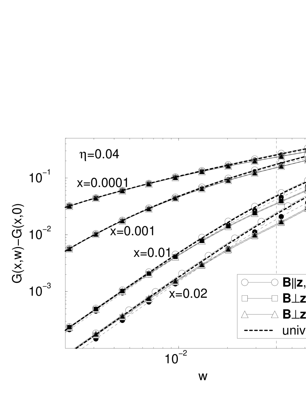
FIG. 4.: Magnetoconductivity scaled according to (86) for various temperatures. We investigate both quasi $1D$- and quasi $2D$-systems. The open and filled symbols denote the conductivity parallel and perpendicular to the planes, respectively. For low magnetic field and low temperatures the effects of WL are universal and do not depend on $\eta$ or the structure of the material, corrections are of the order of $w/\eta$ or $x/\eta$. The thick dashed line is the universal result for a three-dimensional system. All curves of the plot are given for $\eta=0.04$. The universal behavior for $x,w\ll\eta$ is independent of $\eta$.

Actually, we think that exploiting the universality at low temperatures and magnetic field might serve as a valuable tool to analyze experimental results. E.g. leading corrections to the universal behavior show up in powers of $w_{\|/\perp}\,/\eta$ or $x/\eta$ which allows the determination of $\eta$ but also of $x=\tau_{\rm el}/\tau_{\varphi}$.

The absolute size of the WL-correction is for a three-dimensional system always non-universal, i.e. it depends on the behavior of the system on the short length scale $\l_{\rm el}$. A more well-suited quantity is e.g. $(\sigma(T,{\bf B})-\sigma(0,0))/\sigma(0,0)$ which for a generic anisotropic three dimensional system with diffusion constants $D_{x}$, $D_{y}$, $D_{z}$ has for low temperatures and low magnetic field the generic form:

$$\frac{\sigma(T,{\bf B})-\sigma(0,0)}{\sigma(0,0)} = \frac{\tau_{\rm el}}{\pi N_{0}\sqrt{D_{x}D_{y}D_{z}\tau_{\rm el}^{3}}}\,G(x,w)$$ (86)

$$= \frac{1}{4\pi^{2}N_{0}\sqrt{D_{x}D_{y}D_{z}}}\,\sqrt{\frac{x}{\tau_{\rm el}}}g\left(\frac{w}{x}\right)$$ (87)

$$w^{2}=\left(\frac{2e\tau_{\rm el}}{c}\right)^{2}\left(D_{x}D_{y}B_{z}^{2}+D_{y}D_{z}B_{x}^{2}+D_{z}D_{x}B_{y}^{2}\right)$$ (88)

$g(z)$ is a universal function [17] with $g(0)=1$ and $g(z)\to(\zeta(1/2)/2)(1-\sqrt{2})\sqrt{z}\approx 0.3024\sqrt{z}$ for $z\to\infty$. Note that (86) is independent of the cutoff scale $\tau_{\rm el}$.

It is easy to check that for $w_{\|/\perp},x\ll\eta$ all our results for all directions of the current and the magnetic field, and for both the quasi one- and two-dimensional case can be written in this way. In Fig. 4 we have scaled the magnetoconductivity in the above described way – all curves collapse on a single line for $w,x\ll\eta$, signalizing the dominating three dimensional behavior. With the help of (86) it is also possible to scale the universal part to a single line independent of $x$ and $\eta$.

In an experiment it would be very interesting to study systematically the deviations from the $3D$-universality. In the universal $3D$ regime the WL corrections do not depend on the direction of the current and the dependence on the direction of the magnetic field is fully described by the ${\bf B}$-dependence of $w$. Therefore deviations are studied best looking at ratios of conductivities. E.g. without a magnetic field for low temperatures one could investigate the ratio

$$C(T)=\frac{\sigma^{\|}(T)-\sigma^{\|}(0)}{\sigma^{\perp}(T)-\sigma^{\perp}(0)}.$$ (89)

With $C(0)=\lim_{T\to 0}C(T)$ the ratio $C(T)/C(0)\approx 1+\sqrt{x/(4\eta)}+O(\sqrt{x\eta},x/\eta)$ calculated from (23) and (37) for a quasi $2D$ system measures the leading deviations from universality. Similar information, perhaps with an higher accuracy, one can get from the $B^{2}$-rise of the magnetoconductivity, i.e. from

$$D(T)=\left.\frac{\frac{d^{2}\hfill}{dB^{2}}\sigma_{{\bf B}\|\hat{{\bf z}}}^{\|}(T)}{\frac{d^{2}\hfill}{dB^{2}}\sigma_{{\bf B}\|\hat{{\bf z}}}^{\perp}(T)}\right|_{B=0}.$$ (90)

Using the extrapolation of $D(T)$ towards $T=0$ with $D(0)=C(0)$, one can investigate the behavior of $D(T)/D(0)\approx 1-x/(2\eta)+O(\sqrt{\eta x^{3}},(\eta/x)^{2})$. This correction can be seen in the $\log$-$\log$ plot of the magnetoresistivity shown in Fig. 4, where for $w\to 0$ the curves show a small offset proportional to $x$.

Corrections to the universal $3D$ behavior proportional to powers of $w/\eta$ are harder to investigate systematically. For $w<x$ it is difficult to separate them from $x/\eta$ contributions and the regime $w>x$ is very sensible to small variations of the temperature. In a quasi $2D$ system we propose to compare the in-plane and out-of-plane conductivity for a magnetic field perpendicular to the planes using

$$E(T,B)=\frac{\sigma_{{\bf B}\perp\hat{{\bf z}}}^{\|}(T,B)-\sigma_{{\bf B}\perp\hat{{\bf z}}}^{\|}(T,0)}{\sigma_{{\bf B}\perp\hat{{\bf z}}}^{\perp}(T,B)-\sigma_{{\bf B}\perp\hat{{\bf z}}}^{\perp}(T,0)}$$ (91)

as theoretical uncertainties are minimal for this quantity. $E(T,B)$ rises quadratically in $B$ for low fields, but for low temperatures it should be possible to extract a linear contribution in $B$ in the regime $x<w_{\perp}<\eta$. For $T\to 0$ this rise is proportional to $w_{\perp}/\eta$ allowing a measurement of $\eta$. We find $E(0,B)/E(0,0)\approx 1+0.025(w_{\|}/\eta)(1+O(\sqrt{x/\eta}))+O(x/\eta)$.

The predictions of our paper are relevant for a number of experimentally available systems. In the quasi one-dimensional case, one has to look for systems which stay metallic at low temperatures and do not exhibit a Peierls’ transition or a transition to a superconducting state. This seems to be realized in certain pure iodine oxidized phthalocyanine molecular crystals ($M(pc)I$ with $M=H_{2},Ni,Cu,\dots$) where indeed a dimensional crossover as a function of temperature has been observed [2]. However, measurements of the magnetoresistance did not show deviations from the $B^{2}$ behavior, which would be necessary to analyze the data with our theory. Here investigations at lower temperatures and higher magnetic fields would hopefully allow to test our picture.

Very promising seems to be the investigation of quasi two-dimensional systems which do not show a phase-transition and stay metallic at low temperatures. Especially metal-insulator multilayers can be fabricated in a well-controlled way. All parameters entering our theory, i.e. strength of disorder, anisotropy, bandstructure etc. can be be varied over a large range. A number of experiments in such multilayers [18, 19] have shown signatures of a dimensional crossover from two- to three-dimensional behavior. It is important to study systems with quite strong disorder where WL is enhanced and contributions from other effects like classical magnetoresistance, Shubnikov-de Haas oscillations are suppressed or can be separated.

Especially the comparison of the effect of a magnetic field parallel and perpendicular to the planes would allow to identify e.g. the magnetic field independent contribution $K_{2}$.

Finally we want to give a crude estimation for the required magnetic fields necessary to induce a dimensional crossover in a quasi $2D$ system. $w_{\|}\gg\eta$ in our dimensionless units translates to $B\gg\sqrt{D_{\perp}/D_{\|}}\phi_{0}/(4\pi a^{2})$ with the flux-quantum $\phi_{0}=h/2e=2.07\raisebox{1.29167pt}{$\,\times\,$}10^{-15}\,\mathrm{T}\,\mathrm{m}^{2}$. E.g. for $D_{\perp}/D_{\|}\sim 10^{-3}$ and $a\sim\,10\,\mathrm{\AA}$ this yields $B\gg 5\,\mathrm{T}$. The field perpendicular to the planes can be a factor $\sqrt{D_{\perp}/D_{\|}}\approx 30$ smaller. In multilayer materials much larger values for $a$ can be achieved and correspondingly much weaker magnetic fields should lead to the dimensional crossover discussed in this paper. Note that $a$ enters our estimate quadratically.

VI Conclusions

In this paper we have calculated the dimensional crossover in WL induced by inelastic scattering or a magnetic field, for anisotropic three-dimensional systems. At low temperatures and small magnetic field we recover the results for an anisotropic three-dimensional system as different planes or chains are connected by coherent diffusion processes. However, with increasing temperature, as the phase coherence length gets shorter than the lattice distance, a crossover to the two- or one-dimensional behavior of WL can be observed. A similar effect can be seen for an increasing magnetic field. If a typical diffusion path connecting different planes of chains encloses a flux quantum, coherence is destroyed and a dimensional crossover is induced. This phenomenon depends crucially on the direction of both the applied field and the current. We propose to use the magnetic field dependence as a tool to investigate these quantum-interference effects and the dimensional crossover in detail. As compared to the temperature dependence, the magnetic field has the advantage not to dependent on the uncertainties associated with the phase relaxation mechanism. A main qualitative result of our calculations is that for a magnetic field parallel to the planes of a quasi two-dimensional system WL is not fully suppressed by a magnetic field. A finite contribution remains which has its origin in diffusion processes in the plane which do not enclose magnetic flux. It should be possible to measure this remaining contribution by comparing the magnetoresistance for a magnetic field parallel and perpendicular to the planes.

A generalization of this theory to crossovers e.g. from $D=1$ to $D=2$ is straightforward. We have not discussed the influence of WL on the frequency-dependent conductivity [20] in this paper. The effect of a finite frequency $\omega$ in a microwave experiment ($\omega\tau_{\rm el}\ll 1$) can easily be included by replacing $x=\tau_{\rm el}/\tau_{\varphi}$ by $x-i\omega\tau_{\rm el}$ in our formulas. Such a microwave experiment has the advantage that $\omega$ is a known frequency while $1/\tau_{\varphi}$ is only indirectly accessible.

VII Acknowledgment

We wish to thank Yoonseok Lee and W. P. Halperin for helpful communications. C. M. acknowledges financial support of the German-Israeli Foundation.

REFERENCES

- [1] For a review on localization in disordered electron systems see P. A. Lee and T. V. Ramakrishnan, Rev. Mod. Phys. 57, 287 (1985).
- [2] Y. Lee et al., Europhysics Letters 36, 681 (1996).
- [3] E. Abrahams, P. Anderson, D. Licciardello, and T. Ramakrishnan, Phys. Rev. Lett. 42, 673 (1979).
- [4] L. P. Gor’kov, A. I. Larkin, and D. E. Khmel’nitzkiĭ, JETP Lett. 30, 228 (1979).
- [5] B. Altshuler and A. Aronov, in Electron-Electron Interactions in Disordered Systems, edited by A. Efros and M. Pollak (Elsevier Science Publishers B.V., Amsterdam, North-Holland, 1985), p. 1.
- [6] G. Bergmann, Phys. Rev. B 28, 2914 (1983); G. Bergmann, Phys. Rep. 107, 1 (1984).
- [7] D. Vollhardt and P. Wölfle, in Electronic Phase Transitions, edited by W. Hanke and Y. V. Kopaev (Elsevier Science Publishers B. V., Amsterdam, North-Holland, 1992), p. 1.
- [8] P. Wölfle and R. N. Bhatt, Phys. Rev. B 30, 3542 (1984).
- [9] V. N. Prigodin and Y. A. Firsov, J. Phys. C 17, L979 (1984); Y. A. Firsov, in Localization and Metal Insulator Transition, edited by H. Fritzsche and D. Adler (Plenum Press, New York, 1985).
- [10] É. P. Nakhmedov, V. N. Prigodin, and Y. A. Firsov, JETP Lett. 43, 743 (1986).
- [11] N. Dupuis and G. Montambaux, Phys. Rev. Lett. 68, 357 (1992); N. Dupuis and G. Montambaux, Phys. Rev. B 46, 9603 (1992).
- [12] V. V. Dorin, Phys. Lett. A 183, 233 (1993).
- [13] A. Cassam-Chenai and B. Shapiro, J. Phys. (France) I 4, 1527 (1994); A. Cassam-Chenai and D. Mailly, Phys. Rev. B 52, 1984 (1995).
- [14] A. Schmid, Z. Physik 259, 421 (1973).
- [15] M. Abramowitz and I. Stegun, Handbook of Mathematical Functions (Dover Publications, Inc., New York, 1965).
- [16] I. Zambetaki, Qiming Li, E. N. Economou, and C. M. Soukoulis, Phys. Rev. Lett. 76, 3614 (1996); Qiming Li, C. M. Soukoulis, I. Zambetaki, and E. N. Economou, Localization in Highly Anisotropic Systems, preprint cond-mat/9704104 (1997).
- [17] A. Kawabata, Solid State Commun. 34, 431 (1980); A. Kawabata, J. Phys. Soc. Japan 49, 628 (1980).
- [18] B. Y. Jin and J. B. Ketterson, Phys. Rev. B 33, 8797 (1986).
- [19] D. V. Baxter, G. U. Sumanasekera, and J. P. Carini, J. of Magn. and Magn. Mater. 156, 359 (1996); A. N. Fadnis and D. V. Baxter, J. Phys.: Condens. Matter 8, 1389 (1996).
- [20] G. U. Sumanasekera, B. D. Williams, D. V. Baxter, and J. P. Carini, Phys. Rev. B 50, 2606 (1994).