Dispersity-Driven Melting Transition in Two Dimensional Solids

Abstract

We perform extensive simulations of $10^{4}$ Lennard-Jones particles to study the effect of particle size dispersity on the thermodynamic stability of two-dimensional solids. We find a novel phase diagram in the dispersity-density parameter space. We observe that for large values of the density there is a threshold value of the size dispersity above which the solid melts to a liquid along a line of first order phase transitions. For smaller values of density, our results are consistent with the presence of an intermediate hexatic phase. Further, these findings support the possibility of a multicritical point in the dispersity-density parameter space.

srs.tex     May 15, 1997     draft

PACS numbers: 64.70.Dv,64.60.Cn,02.70.Ns,61.20.Ja,05.70.Fh

Recently there has been considerable interest in what happens to the liquid-solid transition in a system if the constituent particles are not all identical but have different sizes. The question was first raised in the context of colloidal solutions[1], and subsequently addressed for other systems [2, 3, 4]. These studies mainly focused on the effect of size dispersity $\Delta$ on the $P-\rho$ equation of state, where $P$ and $\rho$ denote pressure and density. On increasing $\Delta$ from zero, the density discontinuity at the transition decreases, eventually vanishing at a critical value $\Delta=\Delta_{c}$ above which there is no liquid-solid density discontinuity. This remarkable phenomenon— similar to the effect of temperature $T$ on the conventional liquid-gas phase transition[5]—occurs in both two and three dimensions, and for various forms of interaction potentials and size distributions[4].

These seminal studies leave some questions unanswered. First, what are the structures of the phases? Second, can one pass continuously from solid to liquid “around the critical point” at $\Delta_{c}$, just as one can pass continuously from liquid to gas “around the critical point” at $T_{c}$? A “yes” answer would not be consistent with the common picture of melting as a first order phase transition (which cannot have a critical point because of symmetry mismatch of the two phases [6]). A “no” answer would lead to a natural third question: In the $\Delta-\rho$ parameter space, what is the location and nature of the phase boundary between crystalline and liquid phases? The third question has not gone unnoticed—indeed, Ref. [7] simulates a binary mixture of $108$ “soft” disks, and shows that upon increasing $\Delta$ the crystal undergoes a transition to an amorphous solid at a threshold dispersity $\Delta_{th}$, suggesting that the transition is of first order.

Here we address all three questions by simulating a relatively large system comprised of $N=10^{4}$ Lennard-Jones particles of two different radii in a square box of edge $L_{0}$ with periodic boundary condition. With each particle $i$, we associate a size parameter $\sigma_{i}$, and define the distance scale for the interaction between particles $i$ and $j$ to be $\sigma_{ij}\equiv\sigma_{i}+\sigma_{j}$. We assign to half the particles the value $\sigma_{i}=\sigma_{0}(1+\Delta)$, and to the other half the value $\sigma_{i}=\sigma_{0}(1-\Delta)$. If particles $i$ and $j$ are at a distance $r_{ij}$ smaller than a cutoff distance $r_{c}$, they interact via a “shifted-force Lennard-Jones” potential [8] $\Phi_{ij}=4\epsilon\left[\left(\sigma_{ij}/r_{ij}\right)^{12}-\left(\sigma_{ij}/r_{ij}\right)^{6}\right]+f(r_{ij})$. Here $f(r_{ij})$ is a linear function whose coefficients are chosen such that $\Phi_{ij}$ and its gradient, the force, continuously vanish at $r_{ij}=r_{c}$. Since $\Phi_{ij}$ takes its minimum value at $r_{ij}=R_{ij}\equiv 2^{1/6}\times\sigma_{ij}$, we consider this equilibrium distance to be the sum of the radii of the two particles $i$ and $j$, $R_{ij}=R_{i}+R_{j}$, so the radius of particle $i$ is $R_{i}=2^{1/6}\times\sigma_{i}$ and the average radius is $2^{1/6}\times\sigma_{0}$.

We perform molecular dynamics (MD) simulations using the velocity Verlet integrator method [8]. We record the results in reduced units in which $\sigma_{0}$ is $0.5$, and the Lennard-Jones energy scale $\epsilon$, the particle mass, and Boltzmann constant are all unity. In these units, we choose $r_{c}=2.5$ and the length of each MD time step $\delta t=0.01$. The system is first thermalized at $T=1$, using the Berendsen rescaling method [8], for a period of length $\tau$; typically $\tau=(5\times 10^{4})\delta t$. Then we run the system for an additional period $\tau$ as a constant NVE system (micro-canonical ensemble). We continuously calculate $P,T$ and energy $E$, and we consider the system to be in equilibrium only when the fluctuations of all three quantities are less than $1\%$ of their average values. The thermalization time $\tau$ is chosen to be more than the time it takes for the system to equilibrate.

We define the size dispersity to be the ratio of the size distribution variance to its average [3], which equals $\Delta$ in our model, and we define $\rho\equiv\sum_{i=1}^{N}(\pi R_{i}^{2})/L_{0}^{2}$, the ratio of the total area assigned to the disks to the system area. For each value of $\Delta$, we start by placing the $10^{4}$ particles randomly on the sites of a square lattice of edge $L_{0}\approx 150$; higher density states are obtained by gradually compressing the system by reducing $L_{0}$. Typically the starting density is $\rho=0.7$, and we increase $\rho$ to $1.05$ through approximately $10$ intermediate densities, equilibrating the system at each[9].

We present our results for the state points with $T=1$, $\rho=0.90-1.05$ and $\Delta=0-0.12$. At these densities, the $\Delta=0$ system is a 2D-solid with a triangular order, but at large $\Delta$ the system becomes disordered and a liquid. By probing the translational and orientational order, we determine the phase of each state point and we locate the transition between the two phases. To study translational order, we calculate the total pair correlation function $g(r)$, as well as the partial functions $g_{11}(r)$, $g_{22}(r)$ and $g_{12}(r)$ [8]. Here $g(r)$ is the probability distribution of finding two particles at a distance $r$, and $g_{ij}(r)$ is the same for an $(i,j)$ pair ($i=1$ stands for small and $i=2$ for large particles). We find that all three $g_{ij}(r)$ display behavior similar to $g(r)$, indicating that the system maintains its substitutionally-disordered configuration and does not tend toward de-mixing.

In Fig. 1(a) we show the effect of tuning $\Delta$ on translational order. We observe that the monodisperse ($\Delta=0$) system shows the quasi-long-range translational order expected for a 2D-solid[10], characterized by a power-law decay of the envelope of $g(r)$ and the persistence of the solid structure periodicity up to very large distances. For $\Delta<\Delta_{th}(\rho)$, where $\Delta_{th}(\rho)$ is the threshold value at fixed $\rho$, the solid maintains this quasi-long-range order, although the decay exponent appears to increase somewhat with $\Delta$. For $\Delta>\Delta_{th}(\rho)$, we observe a qualitative change in the structure: the quasi-long-range translational order disappears, and is replaced by an exponential decay of the envelope of $g(r)$, which at very long distances shows the uniform distribution of a structureless liquid. We observe this behavior for all densities between $\rho=0.96$ and $\rho=1.05$, and find that $0.09<\Delta_{th}(\rho)<0.10$ for all $\rho$.

Next we study the local bond orientational order by calculating for each particle $j$ the sixfold orientational order parameter[11]

$$(\psi)_{j}\equiv{1\over z}\sum_{k=0}^{z}e^{i6\theta_{jk}}.$$ (1)

The sum runs over all $z$ nearest neighbors $k$ of $j$, and $\theta_{jk}$ is the angle of the bond joining particles $j$ and $k$ with respect to a fixed axis. We identify the nearest neighbors as the particles that are closer than the location of the first minimum of $g(r)$. The modulus of $(\psi)_{j}$ will be unity if the neighbors form a perfect hexagon around $j$, which occurs for all particles in a triangular lattice, the close-packed configuration of a 2D-solid. For a distorted hexagon or a different polygon, $|(\psi)_{j}|<1$— e.g. for a liquid, the distribution of $|(\psi)_{j}|$ centers around $0.5$ [12].

We define the continuous order parameter field $\psi(\mbox{\bf r})$ as the value of $(\psi)_{j}$ if the position of particle $j$ is $\mbox{\bf r}_{j}=\mbox{\bf r}$, and we calculate the orientational correlation function[13]

$$g_{6}(|\mbox{\bf r}-\mbox{\bf r}_{0}|)\equiv\langle\psi(\mbox{\bf r})\psi(\mbox{\bf r}_{0})\rangle,$$ (2)

where $\langle...\rangle$ denotes an average over $\mbox{\bf r},\mbox{\bf r}_{0}$ and time. Fig. 1(b) shows that if $\Delta$ is small and $\rho$ is large, the system displays the long-range orientational order of a solid in that $\lim_{r\rightarrow\infty}g_{6}(r)\neq 0$. Noteworthy is that for each value of $\rho$, orientational order disappears upon a small increase in dispersity near $\Delta_{th}(\rho)$. For $\Delta>\Delta_{th}(\rho)$, $g_{6}(r)$ appears to decay exponentially, which identifies the system as a liquid. Similar plots for other large values of $\rho$ suggest that near $\rho=1.0$, there is a first order phase transition from solid to liquid, driven by an increase in $\Delta$. This observation is in agreement with the results of Ref. [7]. Fig. 1 shows that the small dispersity system has the ordered structure of a solid while the large dispersity system has the disordered structure of a liquid—providing an answer to the first of the three questions.

Since identifying phases relies on the behavior of the system in the thermodynamic limit, we apply finite size scaling to the moments of the orientational order parameter $\psi$, which is the average value of $\psi(\mbox{\bf r})$. We use standard techniques originally developed for the Ising model [14], and recently applied to the 2D melting transition [15, 16]. In order to calculate the moments of $\psi$ at a scale ${b}\equiv L_{0}/M$, we divide the system into $M^{2}$ blocks of edge ${b}$ and we define $\psi_{b}$ for each block as the absolute value of the average of $\psi(\mbox{\bf r})$ over the block. Then we find the moments of $\psi_{b}$ by averaging over all blocks and all configurations of the system after equilibration[15].

To explore the precise location of the phase transition, we calculate the cumulant [15]

$$U_{b}\equiv 1-{{\langle\psi_{b}^{4}\rangle}\over{3\langle\psi_{b}^{2}\rangle^{2}}}.$$ (3)

For a completely ordered (solid) system, $U_{b}=2/3$ in the thermodynamic limit, while for a disordered (liquid) system $U_{b}\rightarrow 0$. For an infinite system, $U_{b}$ jumps between these two limiting values at the phase transition point and for finite systems, this jump becomes rounded. Still, one can determine the location of a phase transition by finding the point at which the $U_{b}$ curves for different system sizes intersect [15]. In Fig. 2, we plot $U_{b}$ versus $\Delta$, for different scales ${b}$ at a fixed $\rho$. We find the transition from the value $2/3$ to lower values upon passing through the phase transition. Moreover, we estimate $\Delta_{th}(\rho)$ from the crossing point of the curves. In the phase diagram of Fig. 3, the line $L_{th}$ is the locus of all such threshold points separating solid and liquid phases and shows that for $\rho>0.96$, $\Delta_{th}(\rho)\approx 0.097$ is essentially independent of $\rho$.

Next we study the finite size scaling of $\langle\psi^{2}_{b}\rangle$. Because of the qualitative difference in the form of $g_{6}(r)$ between solid and liquid, the behavior of $\langle\psi^{2}_{b}\rangle$ as a function of ${b}$ changes drastically upon melting [16]. In the liquid for ${b}\gg\xi$, where $\xi$ is the correlation length, $\langle\psi^{2}_{b}\rangle$ decays as ${b}^{-2}$, while for the solid, $\langle\psi^{2}_{b}\rangle$ remains constant. Fig. 4(a) shows that for $\rho=1.0$, the behavior of the system changes abruptly from solid (given by the line with zero slope) to liquid at $\Delta_{th}$, which is consistent with our previous studies of $g(r)$, $g_{6}(r)$ and $U_{b}$. The $\Delta=0.10$ liquid curve shows long-range correlation for ${b}<\xi$, which crosses over to short-range correlation (slope $-2$) for ${b}\gg\xi$ ($\xi\approx 0.6L_{0}$ for this curve). The corresponding plots for larger $\Delta$ show that $\xi$ shrinks upon increasing $\Delta$. For $\rho=0.9$ (Fig. 4(b)), we observe both solid behavior for $\Delta<0.06$ and liquid behavior for $\Delta>0.06$. For $\Delta=0.06$, Fig. 4(b) shows an algebraic decay for the correlation function, with exponent $-1/4$. This “intermediate” behavior is reminiscent of the hexatic phase[16], for which the orientational correlation decays algebraically while the system does not possess quasi-long-range translational order. In Fig. 3 we have specified as the $I$ phase the locus of the points showing this intermediate behavior.

In summary, we have studied a melting transition driven not by $T$ but by $\Delta$. We have simulated relatively large systems and applied finite size scaling (Figs 2, 4) arriving at a phase diagram for this dispersity-driven melting (Fig. 3). Melting takes place from a 2D ordered phase to a disordered liquid phase, similar to the conventional temperature-driven melting processes. Moreover, at large values of $\rho$, melting is a first order phase transition at a threshold dispersity value $\Delta_{th}(\rho)=0.097\pm 0.005$. Our study of the mean square displacement of the particles shows that this melting is accompanied by a transition from a frozen solid to a diffusive liquid, distinguishing it from the glass transition observed in [7]. The threshold line $L_{th}$ extends almost horizontally down to the point $C$ with coordinates $\Delta_{c}\approx 0.097,\rho_{c}\approx 0.96$. Below $\rho_{c}$, finite size scaling of the orientational order parameter suggests the existence of an intermediate “hexatic” phase between the solid and liquid phases. Thus we hypothesize that point $C$ is a multicritical point, where two lines of continuous transitions (separating liquid/“hexatic” and “hexatic”/solid phases) meet the line of first order transitions $L_{th}$ (separating liquid/solid phases) as shown in Fig. 3[17]. Fig. 3 provides an answer to the last two of the three questions: one can not pass continuously from solid to liquid “around the critical point” $C$, because the two phases are separated by the line of first order phase transitions $L_{th}$. A similar horizontal line of order-disorder transition has been observed in the study of the effect of quenched impurities on the structure of 2D-solids [18].

We thank N. Ito for generously introducing us to this topic, S. T. Harrington for significant assistance in the formative stages of this research, J. L. Barrat for bringing Ref.[7] to our attention, L. A. N. Amaral, N. Clark, W. Kob, B. Kutnjak-Urbanc and D. R. Nelson for extremely helpful criticism, NSF for financial support and the Boston University Center for Computational Science for computational resources.

   

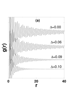
FIG. 1.: Effect of dispersity $\Delta$ on translational and orientational order at $\rho=1.0$. (a)Total pair correlation function $g(r)$ as a function of distance $r$. All curves oscillate around the value $g(r)=1$, so we have separated them to facilitate comparison. We find that a transition from solid to liquid structure occurs on increasing the dispersity between $\Delta=0.09$ and $\Delta=0.10$. (b) Normalized orientational correlation function versus $r$. The change between $\Delta=0.09$ and $\Delta=0.10$ corresponds to the transition from an orientationally long-range correlated solid to a short-range correlated liquid. Both sets of curves show that for $\rho=1.0$ the solid-liquid transition occurs at a value of dispersity between $0.09$ and $0.10$ which is consistent with the observations based on Figs. $2-4$.

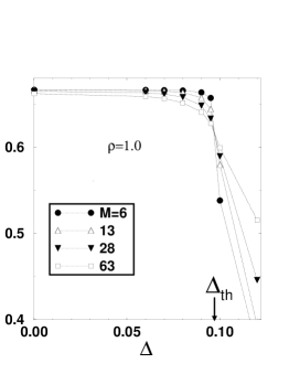
FIG. 2.: Cumulant $U_{b}$ of the bond orientational order parameter $\psi$ as a function of dispersity $\Delta$ for $\rho=1.0$. Different curves correspond to different scales ${b}$, where ${b}\equiv L_{0}/M$ is the block size, so smaller $M$ corresponds to larger scale. The dotted lines connecting the data points are guides to the eye. We identify the threshold value of $\Delta$ to be the point where all the curves for different scales intersect.

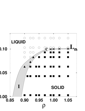
FIG. 3.: Phase diagram in the $\Delta-\rho$ (dispersity-density) parameter space. Squares represent solid points and circles liquid points. The threshold line $L_{th}$ connects crosses, which are the first order phase transition points derived from the cumulant analysis. The triangles are the points of the intermediate ($I$) phase, showing a hexatic behavior. The large diamond marks the multicritical point $C$.

  

FIG. 4.: Log-log plots of $\langle\psi^{2}_{b}\rangle$ versus ${b}$ for different dispersities $\Delta$. Both axes are normalized by their values at system size $L_{0}$, which causes the curves to meet at the origin and facilitates comparing their asymptotic slopes. Dashed lines connecting the data points are guides to the eye. Solid straight lines are reference lines with slopes $-2$ and $-1/4$. (a) For $\rho=1.0$ there is an abrupt change from asymptotic slope of $0$ (data lying on the abscissa) to $-2$, which corresponds to a solid-liquid transition on increasing the dispersity above $\Delta_{th}$. (b) For $\rho=0.9$, the $\Delta=0.06$ curve falls between the solid and liquid regimes, and shows a slope of $-1/4$ characteristic of the hexatic phase.

REFERENCES

- [1] E. Dickinson, Chem. Phys. Lett. 57, 148 (1978); J. Chem. Soc. Faraday II 75, 466 (1979); E. Dickinson and R. Parker, Chem. Phys. Lett. 79, 578 (1981); E. Dickinson, J. Phys. Lett. (France) 46, L29 (1985).
- [2] J. L. Barrat and J. P. Hansen, J. Phys. (France) 47, 1547 (1986).
- [3] P. N. Pusey, J. Physique 48, 709 (1987).
- [4] W. Vermöhlen and N. Ito, Phys. Rev. E 51, 4325 (1995); N. Ito, Int. J. Mod. Phys. C7, 275 (1996).
- [5] Note that is not a thermodynamic control parameter like , but is a geometric parameter which changes the interaction Hamiltonian. In this respect, is similar to bond or site concentration in a diluted Ising model, which modifies the phase diagram and changes the position of the phase transition (see e.g. A. Coniglio, Phys. Rev. Lett. 46, 250 (1981)).
- [6] L. D. Landau and E. M. Lifshitz, Statistical Physics, Translated by J. B. Sykes and M. J. Kearsley, 3rd ed. (Pergamon Press, 1980); H. E. Stanley, Introduction to Phase Transitions and Critical Phenomena (Oxford University Press, New York, 1971).
- [7] L. Bocquet, J. P. Hansen, T. Biben and P. Madden, J. Phys. Cond. Matt. 4, 2375 (1992).
- [8] M. P. Allen and D. J. Tildesley, Computer Simulation of Liquids (Oxford University Press, New York, 1989).
- [9] The average simulation speed on Boston University’s SGI power challenge array is per particle update, so each of the state points studied here requires hours on one processor (over hours total computational time).
- [10] D. R. Nelson, in Phase Transitions and Critical Phenomena, Vol. 7, edited by C. Domb and J. L. Lebowitz (Academic, London, 1983).
- [11] D. R. Nelson and B. I. Halperin, Phys. Rev. B 21, 5312 (1980).
- [12] M. A. Glaser and N. A. Clark, in Geometry and Thermodynamics, edited by J. C. Tolédano (Plenum Press, New York, 1990), p. 193; M. A. Glaser, N. A. Clark, A. J. Armstrong and P.D. Beale, in Dynamics and Patterns in Complex Fluids, edited by A. Onuki and K. Kawasaki (Springer-Verlag, Berlin, 1990), p. 141.
- [13] D. Frenkel and J. P. McTague, Phys. Rev. Lett. 42, 1632 (1979); J. P. McTague, D. Frenkel and M. P. Allen, in Ordering in Two Dimensions, edited by S. K. Sinha (North-Holland, New York, 1980), p. 147.
- [14] K. Binder, Z. Phys. B 43, 119 (1981).
- [15] H. Weber, D. Marx and K. Binder, Phys. Rev. B 51, 14636 (1995).
- [16] K. Bagchi, H. C. Andersen and W. Swope, Phys. Rev. Lett. 76, 255 (1996); Phys. Rev. E 53, 3794 (1996).
- [17] A similar phase diagram has been observed for the conventional (temperature-driven) melting transition of dislocation vector systems, in which the nature of the transition depends on the core energy of the dislocations. These studies show that at large , melting takes place through the formation of the hexatic phase, whereas for small the transition is predominantly first order. The resulting phase diagram in the parameter space is similar to our phase diagram in the parameter space (Fig. 3), with the existence of a multicritical point at the junction of the liquid, hexatic and solid phases. [Y. Saito, Phys. Rev. Lett. 48, 1114 (1982); Phys. Rev B26, 6239 (1982)].
- [18] D. R. Nelson, Phys. Rev. B 27, 2902 (1983); M.-C. Cha and H. A. Fertig, Phys. Rev. Lett. 74, 4867 (1995).