Resonant Raman Scattering in Antiferromagnets

Abstract

Two-magnon Raman scattering provides important information about electronic correlations in the insulating parent compounds of high-$T_{c}$ materials. Recent experiments have shown a strong dependence of the Raman signal in $B_{1g}$ geometry on the frequency of the incoming photon. We present an analytical and numerical study of the Raman intensity in the resonant regime. It has been previously argued by one of us (A.Ch) and D. Frenkel that the most relevant contribution to the Raman vertex at resonance is given by the triple resonance diagram. We derive an expression for the Raman intensity in which we simultaneously include the enhancement due to the triple resonance and a final state interaction. We compute the two-magnon peak height (TMPH) as a function of incident frequency and find two maxima at $\omega^{(1)}_{res}\approx 2\Delta+3J$ and $\omega^{(2)}_{res}\approx 2\Delta+8J$. We argue that the high-frequency maximum is cut only by a quasiparticle damping, while the low-frequency maximum has a finite amplitude even in the absence of damping. We also obtain an evolution of the Raman profile from an asymmetric form around $\omega^{(1)}_{res}$ to a symmetric form around $\omega^{(2)}_{res}$. We further show that the TMPH depends on the fermionic quasiparticle damping, the next-nearest neighbor hopping term $t^{\prime}$ and the corrections to the interaction vertex between light and the fermionic current. We discuss our results in the context of recent experiments by Blumberg et al. on $Sr_{2}CuO_{2}Cl_{2}$ and $YBa_{2}Cu_{3}O_{6.1}$ and Rübhausen et al. on $PrBa_{2}Cu_{3}O_{7}$ and show that the triple resonance theory yields a qualitative and to some extent also quantitative understanding of the experimental data.

]

I Introduction

In recent years a lot of efforts have been undertaken to understand the pairing mechanism in high-$T_{c}$ superconductors [1, 2, 3]. Some of the existing theories consider an effective electron-electron interaction mediated by spin fluctuations as the source of the pairing mechanism [4, 5]. In the parent compounds of the high-$T_{c}$ materials the strong magnetic correlations lead to the occurrence of antiferromagnetism. Two-magnon Raman scattering is a valuable tool in probing antiferromagnetism and can thus provide important insight into the nature of the pairing correlations [6, 7, 8, 9].

The two-magnon Raman scattering cross section (Raman intensity) is proportional to the Golden Rule transition rate [10]

$$R={8\pi^{3}e^{4}\over\hbar^{3}V^{2}\omega_{i}\omega_{f}}\sum{|M_{R}|^{2}\delta(\hbar\omega_{i}-\hbar\omega_{f}+\epsilon_{i}-\epsilon_{f})}$$ (1)

where $i$ and $f$ are the initial and final states of the system, $\epsilon_{i,f}$ are the corresponding energies and ($\epsilon_{i}-\epsilon_{f}$) is the total energy of the two magnons in the final state. $M_{R}=<\hat{e}_{f}^{*}|M_{R}|\hat{e}_{i}>$ is the Raman matrix element (Raman vertex), $\hat{e}_{i}$ and $\hat{e}_{f}$ are the polarization unit vectors of the incident and outgoing photons, and the summation runs over all possible initial and final electronic states.

Graphically, the Raman intensity is given by the diagram shown in Fig. 1a, where the intermediate magnons (wavy lines) are on the mass shell. The dashed lines in this diagram describe the incident and outgoing photons and the shaded circles represent the full Raman vertices, which include all effects of the final state magnon-magnon interaction [11].

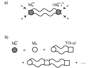
FIG. 1.: (a) The Raman cross section is proportional to this diagram where the intermediate magnons (wavy lines) are on the mass shell. The dashed lines present incoming and outgoing photons and the filled circles are the full Raman vertices $M_{R}^{tot}$. (b) The full Raman vertices include all effects of multiple magnon-magnon scattering. The open circles are the bare Raman vertices $M_{R}$ and the open squares describe the magnon-magnon scattering vertex $V(k,q)$.

In conventional Raman experiments, one measures the Raman intensity, $R$, as a function of transferred photon frequency $\Delta\omega=\omega_{i}-\omega_{f}$ where $\omega_{i}$ and $\omega_{f}$ are the incident and outgoing photon frequencies, respectively. The fingerprint of antiferromagnetism in these experiments is the presence of a two-magnon peak in $R(\Delta\omega)$ [12]. In the insulating parent compounds of the high-$T_{c}$ materials, this peak occurs at a transferred frequency of about $3000cm^{-1}$. The two-magnon peak has not only been observed in the insulating compounds, but also in electron [13] and hole doped materials [14].

Theoretically, most of the analytical and numerical studies of two-magnon Raman scattering were performed within the conventional phenomenological Loudon-Fleury (LF) theory [15] which assumes that the matrix element $M_{R}$ for the interaction between photons and magnons is frequency independent. This implies that the theory neglects the internal structure which the matrix element possesses since the spin-photon interaction is actually mediated by fermions: the incident photon creates a particle-hole pair which emits two spin excitations and annihilates into an outgoing photon (see e.g., Fig. 2).

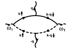
FIG. 2.: The triple resonance diagram which yields the dominant contribution to the Raman intensity in the resonant regime. Solid and dashed lines represent fermions from conduction and valence bands, respectively. Notice that this diagram contains intraband scattering at the fermion-magnon vertices.

Despite this weakness, the LF theory was originally considered as a suitable theory for Raman scattering in the parent high-$T_{c}$ materials because it predicts that the two-magnon profile should have a peak at a transferred frequency of about $2.8J$ where $J$ is the magnetic exchange interaction. A comparison with the data [12, 16, 17] then yields $J=0.12eV$ which is fully consistent with the value for the in-plane exchange interaction extracted from neutron scattering [18] and NMR data [19].

Recent experiments on single-layer $Sr_{2}CuO_{2}Cl_{2}$ and double-layer $YBa_{2}Cu_{3}O_{6.1}$[20] as well as on $PrBa_{2}Cu_{3}O_{7}$[21], however, presented some qualitative features of the Raman signal which cannot be explained within the framework of the LF theory. In these experiments, the Raman intensity was measured both as a function of transferred frequency at a given incident frequency $\omega_{i}$ (the two-magnon profile), and as a function of $\omega_{i}$ at a fixed transferred frequency $\Delta\omega\approx 2.8J$ at which the two-magnon profile exhibits a maximum. In the latter case one in fact measures the variation of the two-magnon peak height (TMPH) with $\omega_{i}$. The experimental features which are in disagreement with the LF theory include:
$1)$ A strong dependence of the TMPH on $\omega_{i}$ with two distinct maxima at $\omega_{i}=\omega^{(1)}_{res}\approx 2\Delta+3J$ and at $\omega_{i}=\omega^{(2)}_{res}\approx 2\Delta+8J$, where $2\Delta\sim 1.7eV$ is the charge transfer gap [22]. Despite quantitative differences between various compounds, the second maximum in all compounds is always stronger than the first one. The LF theory, on the contrary, predicts that the intensity should only undergo a weak (logarithmical) enhancement at $\omega_{i}=2\Delta$ and $\omega_{i}=2\Delta+2.8J$ (ingoing and outgoing resonances). No enhancement, however, has been experimentally observed at $\omega_{i}=2\Delta$.
$2)$ The shape of the two-magnon profile is asymmetric and possesses a shoulder-like feature for transferred frequencies above the two-magnon peak, i.e., for $\Delta\omega>2.8J$. This feature has been observed around the first resonance at $\omega_{res}^{(1)}$; it practically disappears when the frequency of the incident photon approaches the second resonance at $\omega_{res}^{(2)}$.

Motivated by these findings, several groups studied two-magnon Raman scattering beyond the LF approximation [23, 24, 25]. It has been shown that the validity of the LF theory is restricted to the nonresonant regime, when the frequency of the incident light is much smaller than the charge-transfer gap $2\Delta$ [23, 24]. Most of the experiments, however, are performed with photon frequencies slightly above the charge transfer gap. In this resonant regime the internal structure of the Raman matrix element cannot be neglected. Chubukov and Frenkel (hereafter referred to as CF) developed a diagrammatic approach to Raman scattering in the framework of the large-$U$ spin-density-wave (SDW) approach to the Hubbard model at half-filling [24]. They identified those diagrams which reproduce the LF vertex, and in addition identified a new diagram which is not included in the LF theory but yields the dominant contribution to the scattering process in the resonant regime. This new diagram has the largest amplitude when $|\omega_{i,f}-2\Delta|=O(J)$, and in addition, diverges in the absence of a fermionic damping in a small region (nearly a single critical line) in the $(\omega_{i},\Delta\omega)$ plane where all three terms in the denominator vanish simultaneously (see Fig. 3). Due to this property, the new diagram identified by CF is called the triple resonance diagram. The inclusion of a fermionic damping eliminates the divergence, but the Raman matrix element remains strongly peaked along the critical line.

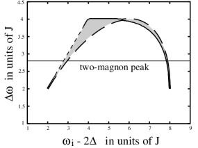
FIG. 3.: The shaded area represent the region in the $(\omega_{i},\Delta\omega)$ plane in which the triple resonance occurs. The horizontal line corresponds to $\Delta\omega=2.8J$ at which the two-magnon profile has a peak.

Since the computation of the full Raman intensity with the triple diagram for the Raman vertex is rather involved, CF used a semi-phenomenological approach to analyze the dependence of the TMPH on $\omega_{i}$. They considered the final state magnon-magnon interaction and the triple resonance enhancement separately, and conjectured that the experimentally observed two maxima in the TMPH occur at $\omega_{i}$ for which the Raman vertex resonates at the same transferred frequency $\Delta\omega=2.8J$ at which the two-magnon profile has a peak. By analyzing where the resonant line for the Raman vertex crosses $\Delta\omega=2.8J$, they obtained two resonance frequencies, $\omega^{(1)}_{res}\sim 2.9J+2\Delta$ and $\omega^{(2)}_{res}\sim 7.9J+2\Delta$ which both agree with the experimental data.

The analysis in Ref. [24], however, left several issues open. First, the validity of the semi-phenomenological approach needs to be verified. Second, the quantitative behavior of the TMPH as a function of $\omega_{i}$ and, in particular, the form of the peaks at $\omega^{(1)}_{res}$ and $\omega^{(2)}_{res}$ and their relative amplitudes have not been studied yet. CF merely conjectured, without performing explicit calculations, that the resonance at $\omega_{res}^{(1)}$ should be weaker than the one at $\omega^{(2)}_{res}$ because near $\omega_{res}^{(1)}$, there exists a strong restriction on the possible directions of the magnon momenta which satisfy the resonance condition at a given magnon energy. No such restriction exists near $\omega_{res}^{(2)}$. This conjecture also has to be verified by explicit calculations. Third, the anisotropy of the two-magnon profile and its evolution with varying incident frequency has not been studied. Forth, the calculations in CF were performed in the framework of a mean-field, large $U$, spin-density-wave (SWD) approach to the Hubbard model with only nearest-neighbor hopping. This theory, however, possesses the weakness that it predicts that the maximum of the valence band is degenerate along the boundary of the magnetic Brillouin zone. Meanwhile, experiments on $Sr_{2}CuO_{2}Cl_{2}$ have demonstrated that the valence fermions possess a strong dispersion along the magnetic Brillouin zone boundary with maxima at $(\pi/2,\pi/2)$ and symmetry related points [26, 27]. This dispersion can easily be reproduced in the SDW formalism if one includes a next-nearest-neighbor hopping, $t^{\prime}$. This, however, changes the energy denominator in the triple resonance diagram, and one therefore has to reexamine the conclusions of CF by performing their calculations for the $(t-t^{\prime}-U)$ model. The inclusion of $t^{\prime}$ is particularly relevant for computations near $\omega^{(1)}_{res}$ since the dominant contribution to the Raman vertex in this frequency range comes from fermions near the top of the valence band whose degeneracy is lifted by $t^{\prime}$.

The goal of the present paper is to address the above issues. We will compute below the Raman intensity including both a final state interaction and the enhancement of the Raman vertex due to the triple resonance. We will study the Raman profile and the TMPH numerically and analytically and demonstrate that the two peaks in the TMPH survive the effects of the magnon-magnon interaction. We will analyze the relative amplitude of the TMPH near $\omega^{(1)}_{res}$ and $\omega^{(2)}_{res}$ and show that although the divergent piece near $\omega^{(1)}_{res}$ is much weaker than the one near $\omega^{(2)}_{res}$, the nondivergent term is much larger near $\omega^{(1)}_{res}$. As a result, the relative amplitude of the two peaks in the TMPH turns out to be strongly dependent on the quasiparticle damping which cuts the divergent part but does not affect the subleading term substantially. We will also show that both peaks in the TMPH are anisotropic - the intensity drops much faster on the high-frequency side of each of the peaks. Further, we will study the effects on the TMPH of a next-nearest neighbor hopping $t^{\prime}$ and vertex corrections to the interaction between light and fermionic quasiparticles.

We will also study how the two-magnon lineshape evolves with the incident frequency, and show that it changes from an asymmetric form for $\omega_{i}\geq\omega^{(1)}_{res}$ to a symmetric form around $\omega_{i}\approx\omega^{(2)}_{res}$.

We will compare our results with the experimental data on on $Sr_{2}CuO_{2}Cl_{2}$ and $YBa_{2}Cu_{3}O_{6.1}$ by Blumberg et al. and on $PrBa_{2}Cu_{3}O_{7}$ by Rübhausen et al. and demonstrate that all the features in the two-magnon profile and the TMPH observed in Raman experiments can be qualitatively described by the triple resonance diagram. At the same time, we will see that quantitative agreement with the data is not always perfect.

The paper is organized as follows. In Sec. II, we present the formalism and the expressions for the Raman vertex both in the LF approximation and near the resonance. In Sec. III we present our analytical results for the vertex near $\omega^{(1,2)}_{res}$ and demonstrate that the divergence is much stronger near the upper resonance frequency. We also discuss in this section how the inclusion of a next-nearest-neighbor hopping $t^{\prime}$ affects the resonance behavior of the Raman vertex. In Sec. IV we present our numerical results for (a) the Raman line shape for different incident frequencies $\omega_{i}$ (Sec. IV A) and (b) for the TMPH as a function of $\omega_{i}$ (Sec. IV B). We then discuss its dependence on the fermionic damping and the inclusion of $t^{\prime}$ (Sec. IV C). In Sec. IV D we consider vertex corrections to the interaction between light and the fermionic current. Finally, in Sec.V we compare our results with the experimental data.

II The Formalism

The two-magnon Raman scattering cross section is given by Eq.(1). In this paper, we will focus on the $x^{\prime}y^{\prime}$ scattering geometry where most experiments have been performed. In this geometry, the polarization unit vectors of the incident and outgoing light are both real (linearly polarized light), perpendicular to each other and directed at $45^{o}$ to the crystallographic directions, i.e., $\hat{e}_{i}=x^{\prime}=(\hat{x}+\hat{y})/\sqrt{2},\hat{e}_{f}=y^{\prime}=(\hat{x}-\hat{y})/\sqrt{2}$. Other scattering geometries for linearly polarized light are $x^{\prime}x^{\prime}$ where $\hat{e}_{i}=\hat{e}_{f}=(\hat{x}+\hat{y})/\sqrt{2}$, $xy$ where $\hat{e}_{i}=\hat{x},\hat{e}_{f}=\hat{y}$ and $xx$ where $\hat{e}_{i}=\hat{x},\hat{e}_{f}=\hat{x}$. For circularly polarized light, the scattering geometries are LL where $\hat{e}_{i}=\hat{e}_{f}=(\hat{x}+i\hat{y})/\sqrt{2}$, and LR where $\hat{e}_{i}=(\hat{x}+i\hat{y})/\sqrt{2},\hat{e}_{f}=(\hat{x}-i\hat{y})/\sqrt{2}$.

The $x^{\prime}y^{\prime}$ geometry is often referred to as the $B_{1g}$ geometry. Strictly speaking the matrix element in the $x^{\prime}y^{\prime}$ scattering channel includes $B_{1g}$ and $A_{2g}$ components with $M^{B_{1g}}_{R}=<x|M_{R}|x>-<y|M_{R}|y>$ and $M^{A_{2g}}_{R}=<x|M_{R}|y>-<y|M_{R}|x>$. In practice, however, the $A_{2g}$ component is always negligible, and we will therefore not distinguish between $x^{\prime}y^{\prime}$ and pure $B_{1g}$ scattering.

As we already discussed in the introduction, we will consider Raman scattering in the framework of the large-$U$ SDW formalism for the one-band Hubbard model. In this approach, one introduces a long-range antiferromagnetic order and decouples the electronic dispersion into two subbands of valence and conduction fermions.

The diagrammatic approach to the Raman scattering in the SDW formalism was developed by CF. An example for the diagrams which contribute to the bare Raman vertex is shown in Fig. 2. This diagram contains two types of vertices: one for the interaction between fermions and light, and one for the interaction between fermions and magnons. The interaction with light appears in the SDW theory as a result of the modulation of the hopping matrix element by the vector potential of the electromagnetic field. The spin-fermion vertices can be straightforwardly obtained from the full expression of the spin susceptibility which in the SDW theory is given by the RPA series of bubble diagrams. In each of theses bubbles one fermion is from the valence band and the other is from conduction band.

To obtain the Raman intensity, we need to know the full Raman vertex which includes a whole series of magnon-magnon interaction events. It has already been emphasized several times in the literature that the dominant contribution to the magnon-magnon scattering comes from the region near the magnetic Brillouin zone boundary where the antiferromagnetic magnons behave almost as free particles [11, 28]. In this situation, the only relevant interaction term has two creation and two annihilation magnon operators:

$${\cal H}_{int}=-\frac{4J}{N^{2}}{\sum_{k}}{\sum_{q}}\nu_{k-q}a^{\dagger}_{k}\beta^{\dagger}_{-k}\beta_{-q}a_{q}.$$ (2)

We can now decompose the interaction vertex into

$$\nu_{k-q}=\nu_{k}\nu_{l}+{\tilde{\nu}}_{k}{\tilde{\nu}}_{l}+{\bar{\nu}}_{k}{\bar{\nu}}_{l}+{\bar{\tilde{\nu}}}_{k}{\bar{\tilde{\nu}}}_{l}\;.$$ (3)

where the different symmetry factors are given by

$$\nu_{k} = \frac{1}{2}(\cos k_{x}+\cos k_{y});~{}~{}~{}~{}\tilde{\nu}_{k}=\frac{1}{2}(\cos k_{x}-\cos k_{y});$$ (4)

$$\bar{\nu}_{k} = \frac{1}{2}(\sin k_{x}+\sin k_{y});~{}~{}~{}~{}\bar{\tilde{\nu}}_{k}=\frac{1}{2}(\sin k_{x}-\sin k_{y}).$$ (5)

Before we discuss our calculations for the full Raman intensity at resonance, we briefly review the calculation of the Raman intensity in the nonresonant regime when the LF theory is valid. In the LF theory, the bare Raman vertex (open circle in Fig. 1b) is assumed to be independent of the photon frequencies while its dependence on the magnon momentum $q$ has the form [23, 24]

$$M_{R} = A~{}\Big{[}\nu_{q}(e_{ix}e^{*}_{fx}+e_{iy}e^{*}_{fy})$$

$$\quad-(e_{ix}e^{*}_{fx}\cos q_{x}+e_{iy}e^{*}_{fy}\cos q_{y})\Big{]}\ ,$$

where $A$ is a constant. In the diagrammatic approach, the LF vertex is obtained by collecting the diagrams with interband scattering at the magnon-fermion vertices. At photon frequencies small compared to the SDW gap, these diagrams have the largest overall factor. One can easily check that $M_{R}$ is finite only in the $B_{1g}$ scattering geometry and for LR polarized light. In both cases we obtain $M_{R}=-A\tilde{\nu}_{q}$. For this particular form of $M_{R}$, only the second term in Eq.(3) contributes to the magnon-magnon scattering process. With this simplification, the summation of the ladder series for the full Raman intensity can be reduced to solving an algebraic equation. Doing this we obtain for the full Raman intensity in the $B_{1g}$ channel

$$R(\omega)\propto Im\left[\frac{I}{1+I/4S}\right]\ ,$$ (6)

where $S$ is the value of the spin, and

$$I=\frac{4JS}{N}{\sum_{q}}\frac{(\cos q_{x}-\cos q_{y})^{2}}{\Delta\omega-2\omega_{q}+i\delta}$$ (7)

with $\Delta\omega=\omega_{i}-\omega_{f}$ and $\omega_{q}=4JS\sqrt{1-\nu^{2}_{q}}$ is the magnon dispersion. Eqs.(6) and (7) yield a two-magnon peak at $\Delta\omega=2.8J$ (for $S=1/2$), but $R(\omega)$ clearly contains no dependence on the incident photon frequency $\omega_{i}$ [11, 15].
As mentioned earlier, the LF theory is only valid for small $\omega_{i}$. When $\omega_{i}$ is comparable to the gap between the conduction and valence bands (which in the cuprates is the charge transfer gap), it turns out that diagrams with intraband scattering at the fermion-magnon vertices (in contrast to interband scattering in the LF diagrams) become dominant. The most relevant of these diagrams is shown in Fig. 2. This diagram is called the triple resonance diagram because it contains three terms in the denominator which can all vanish simultaneously if we adjust the incident and final photon frequencies. The analytical expression for this diagram is given by

$$M_{R}=-{4i\over N}{\sum_{k}}^{\prime}{\Big{(}\displaystyle{\partial\epsilon_{k}\over\partial k}e_{i}\Big{)}\Big{(}\displaystyle{\partial\epsilon_{k-q}\over\partial k}e_{f}\Big{)}\Big{[}\mu_{q}\epsilon_{k-q}-\lambda_{q}\epsilon_{k}\Big{]}^{2}\over\Big{(}\omega_{i}-2E_{k}+i\Gamma\Big{)}\Big{(}\omega_{f}-2E_{k-q}+i\Gamma\Big{)}}$$ (8)

$$\quad\times\Bigg{\{}{1\over\Big{(}\omega_{i}-\omega-E_{k}-E_{k-q}+i\Gamma\Big{)}}$$ (9)

$$\qquad+{1\over\Big{(}\omega_{f}+\omega-E_{k}-E_{k-q}+i\Gamma\Big{)}}\Bigg{\}}\ ,$$ (10)

where $\omega$ is the external magnon frequency,

$$\epsilon_{k} = -2t(\cos{k_{x}}+\cos{k_{y}})=-4t\nu_{k},\ E_{k}=\sqrt{\Delta^{2}+\epsilon_{k}^{2}}\ ,$$

$$\mu_{q} = \Bigg{[}{1\over 2}\Bigg{(}{1\over\sqrt{1-\nu_{q}^{2}}}+1\Bigg{)}\Bigg{]}^{1\over 2},\ \lambda_{q}=\Bigg{[}{1\over 2}\Bigg{(}{1\over\sqrt{1-\nu_{q}^{2}}}-1\Bigg{)}\Bigg{]}^{1\over 2},$$

and the prime indicates summation over the magnetic Brillouin zone. The $i\Gamma$ term represents the fermionic quasi-particle damping which we assume for simplicity to be independent of momentum. The actual damping, indeed, should have some momentum dependence, particularly near the top of the valence band [29, 30, 31, 32]. Out of the three terms in the numerator, the first two are the vertex functions for the interaction between light and fermions, while the third term is the product of the two vertices for the interaction between fermions and magnons.

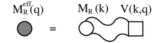
FIG. 4.: The effective Raman vertex $M_{R}^{eff}$ includes a single magnon-magnon scattering event.

As follows from Eq.(10), the resonant Raman vertex $M_{R}$ depends on the magnon momentum, but also, via the denominator, on the incident and outgoing photon frequencies and on the magnon frequency. The frequency dependence of $M_{R}$ can only be eliminated in the artificial limit when the fermionic damping is very large and overshadows all other terms in the denominator. For small and moderate damping, the frequency dependent and also momentum dependent terms in the denominator cannot be ignored, and this makes the computation of the full Raman intensity rather involved. We found, however, that the diagram which is most difficult to compute is the one without a final state interaction. At the same time, the series of diagrams with at least two scattering events can easily be summed up because the Raman vertex renormalized by the inclusion of just a single magnon-magnon scattering event no longer depends on the magnon frequency while its dependence on the external magnon momentum $l$ reduces to a simple $\tilde{\nu}_{l}$ form for $B_{1g}$ scattering. This effective Raman vertex, $M^{eff}_{R}=\tilde{\nu}_{l}\,\bar{M}^{eff}_{R}$ is shown in Fig. 4.

We remind that the experimentally measured Raman profile for any incident photon frequency contains a prominent two-magnon peak which is solely due to magnon-magnon scattering. In this situation, the diagrams without and with a single magnon-magnon scattering are most likely to be less relevant than the diagrams with multiple scattering events. For our analytical considerations, we neglect the diagrams with no or only one magnon-magnon scattering event. In this approximation, we can formally rewrite the full Raman intensity in the same form as for the LF theory:

$$R(\omega_{i},\omega_{f})\propto Im\Bigg{\{}|\bar{M}^{eff}_{R}|^{2}\;\frac{I}{1+I/4S}\Bigg{\}}\ .$$ (11)

where $I$ is the same as in Eq. (7), and $\bar{M}^{eff}_{R}$ is obtained by substituting Eq.(10) into the diagram in Fig. 4 and performing the integration over the intermediate magnon frequency and momenta. We then obtain

$$\bar{M}^{eff}_{R}(\omega_{i},\omega_{f})$$ (12)

$$\qquad=i{128J\over N^{2}}{\sum_{k,q}}^{\prime}{\Big{(}\displaystyle{\partial\epsilon_{k}\over\partial k}e_{i}\Big{)}\Big{(}\displaystyle{\partial\epsilon_{k-q}\over\partial k}e_{f}\Big{)}\Big{[}\mu_{q}\epsilon_{k-q}-\lambda_{q}\epsilon_{k}\Big{]}^{2}\over\Big{(}\omega_{i}-2E_{k}+i\Gamma\Big{)}\Big{(}\omega_{f}-2E_{k-q}+i\Gamma\Big{)}}$$ (13)

$$\qquad\times{\tilde{\nu}_{q}\over\Big{(}\Delta\omega-2\omega_{q}+i\delta\Big{)}\Big{(}\omega_{i}-\omega_{q}-E_{k}-E_{k-q}+i\Gamma\Big{)}}.$$ (14)

It is essential however that $\bar{M}_{R}^{eff}$ still possesses a complex dependence on the external incident and outgoing photon frequencies. This in turn implies that the full intensity $R(\omega_{i},\omega_{f})$ is a function of both frequencies rather than of $\omega_{i}-\omega_{f}$ as in the LF theory. A very similar approach was used by Schönfeld et al. [25].

In our numerical calculations of the full Raman intensity we considered all diagrams, i.e., diagrams with zero, one or multiple magnon-magnon scattering events. The details of this computation are presented in Appendix A. We found a good qualitative agreement between our numerical and analytical results and consider this as a partial justification for the omission of the lowest order diagrams in our analytical considerations.

We now proceed with the discussion of our analytical results, and then present our numerical data.

III Analytical results

In this section, we present the results of our calculations of the Raman intensity near the two resonant frequencies, $\omega^{(1)}_{res}$ and $\omega^{(2)}_{res}$. We first consider the case $t^{\prime}=0$ and then discuss how the intensity changes if we break the particle-hole symmetry by including a hopping term between next-nearest neighbors. Our point of departure is the approximate expression for the Raman intensity, Eq.(11), in terms of the effective Raman vertex, $\bar{M}^{eff}_{R}$. We first study the form of $\bar{M}_{R}^{eff}$ near $\omega^{(2)}_{res}$ and then discuss the form of the vertex near $\omega^{(1)}_{res}$.

A Resonance at $\omega^{(2)}_{res}$

As we discussed in the introduction, the upper resonance frequency, $\omega^{(2)}_{res}$, is close to the maximum possible incident frequency $2\Delta+8J$ for which the resonance condition can still be satisfied (we assume here that $\Delta$ is large, i.e., $E_{k}=\Delta+J(\cos k_{x}+\cos k_{y})^{2}$). The resonance at the highest incident frequency corresponds to a process in which light causes a transition of a quasiparticle from the bottom of the valence band to the top of the conduction band (see Fig. 5).

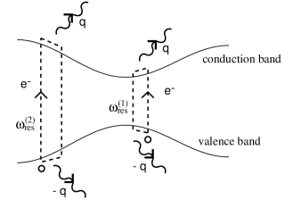
FIG. 5.: Quasiparticles at the bottom of the valence band contribute to the Raman vertex at $\omega_{res}^{(2)}$, whereas quasiparticles at the top of the valence band contribute to $\omega_{res}^{(1)}$. The dashed and wavy lines represent the excited quasiparticles and the emitted magnons, respectively.

Since the bottom of the valence band is at ${\bf k}=(0,0)$ and is not degenerate at the mean-field level, it is reasonable to assume that the corrections to the mean-field fermionic dispersion near the bottom of the band will only give rise to a finite lifetime, but will not introduce any new qualitative features into the fermionic spectrum. We therefore restrict our considerations to the mean-field form of the fermionic dispersion and model the fluctuation effects by introducing a quasiparticle damping $\Gamma$.

To simplify the presentation, we first neglect the numerator in Eq.(14) and focus on the resonance behavior of the effective vertex due to the vanishing denominator. Near the bottom of the band, we can expand the fermionic dispersion and obtain $E_{k}=\Delta+4J-2Jk^{2}$. We will assume that near the resonance the bosonic momentum $q$ is also small such that the expansion near the bottom of the band holds for both $E_{k}$ and $E_{k+q}$. This last assumption will be verified after we perform our calculations. Further, for small $q$ we can expand $\omega_{q}$ as $\omega_{q}=J\sqrt{2}q$. Substituting the expanded forms of $E_{k},E_{k+q}$ and $\omega_{q}$ into Eq.(14), neglecting the numerator, and introducing the dimensionless variables $\lambda_{i}=(\omega_{i}-2\Delta)/2J$ and $\Delta\lambda=\Delta\omega/2J$ we obtain

$${\bar{M}}^{eff}_{R} \propto \int^{\prime}\frac{d^{2}k\;d^{2}q}{(\Delta\lambda-q\sqrt{2}+i\Gamma)}$$ (17)

$$\times{1\over(\lambda_{i}-4+2k^{2}+i\Gamma)(\lambda_{i}-4-\Delta\lambda+2({\vec{k}}-{\vec{q}})^{2}+i\Gamma)}$$

$$\times\;{1\over(2\lambda_{i}-8-\Delta\lambda+2k^{2}+2(\vec{k}-\vec{q})^{2}+(\Delta\lambda-q\sqrt{2})+i\Gamma)}\ .$$

A similar expansion has been performed by CF. They however considered only the bare Raman vertex (the one without a final state interaction) in which case the Golden Rule requires the magnons to be on the mass shell, i.e., $q=q_{0}=\Delta\lambda/\sqrt{2}$. For on-shell magnons, the integration over $d^{2}q$ just yields a factor $2\pi^{2}iq_{0}$. Furthermore, for $q=q_{0}$, the last term in the denominator in Eq.(LABEL:trunk) is the sum of the second and the third term, so one can tune $k$ and the angle between ${\bf k}$ and ${\bf q}$ such that all three terms in the denominator of (LABEL:trunk) vanish simultaneously. Expanding near this point, CF obtained $M_{R}\propto(\lambda_{i}-\lambda_{res})^{-3/2}$.

We now show that the fully renormalized ${\bar{M}}^{eff}_{R}$ possesses the same functional form as the bare vertex obtained by CF since the integration over $q$ by itself is confined to the vicinity of $q_{0}$. To demonstrate this, we expand near the point where the second and the third term vanish and then integrate over ${\bf k}$ and ${\bf q}$. The conditions that the two denominators vanish simultaneously at a given $q$ are $2k^{2}=2k^{2}_{0}=4-\lambda_{i}$ and $\cos\phi=\cos\phi_{0}=(2q^{2}-\Delta\lambda)/(4k_{0}q)$. We will see below that in order to obtain the most singular contribution to $\bar{M}^{eff}_{R}$, one has to expand around $k_{0}$ and $\phi_{0}$ to linear order in $x=k-k_{0}$ and to quadratic order in $y=\phi-\phi_{0}$. Performing this expansion, we obtain

$$\bar{M}^{eff}_{R}\propto\int\frac{d^{2}q\;G(q)}{\Delta\lambda-q\sqrt{2}+i\Gamma}\ ,$$ (19)

where

$$G(q) = \int dx\frac{1}{(x+i\Gamma)(k_{0}x+(\Delta\lambda-q\sqrt{2})/4+i\Gamma)}\times$$ (22)

$$\int dy\Bigg{[}\frac{1}{C_{1}+k_{0}q\sin\phi_{0}y+k_{0}qy^{2}/2+i\Gamma}$$

$$-\frac{1}{C_{2}+k_{0}q\sin\phi_{0}y+k_{0}qy^{2}/2+i\Gamma}\Bigg{]}\ ,$$

and $C_{1}$ and $C_{2}$ are given by

$$C_{1} = x(k_{0}-(2q^{2}-\Delta\lambda)/4k_{0})\ ;$$

$$C_{2} = C_{1}+k_{0}x+(\Delta\lambda-q\sqrt{2})/4\ .$$

The integration over $y$ can be done explicitly and yields

$$G(q) = 2\pi\int\frac{dx}{(x+i\Gamma)(k_{0}x+(\Delta\lambda-q\sqrt{2})/4+i\Gamma)}\times$$ (25)

$$\Bigg{[}\frac{1}{\sqrt{2k_{0}qC_{1}-(k_{0}q)^{2}\sin^{2}\phi_{0}+i\Gamma}}$$

$$-\frac{1}{\sqrt{2k_{0}qC_{2}-(k_{0}q)^{2}\sin^{2}\phi_{0}+i\Gamma}}\Bigg{]}\ .$$

We immediately see that if $\sin\phi_{0}$ is finite, one can expand the square root in the integrand in Eq.(25) in $C_{1,2}$ and find after simple manipulations that the Raman vertex is free from singularities. To obtain a divergent, resonant contribution to the vertex, we therefore have to set $\sin\phi_{0}=0$. For any given $q$, this singles out a line in the $(\lambda_{i},\Delta\lambda)$ plane with

$$\lambda_{i}=\lambda^{(2)}_{res}(q,\Delta\lambda)=4-\frac{q^{2}}{2}\left(1-\frac{\Delta\lambda}{2q^{2}}\right)^{2}\ .$$ (26)

Furthermore, we also have to require that the poles and branch cuts in the integrand in Eq.(25) be in different half-planes, since otherwise, the integral over $x$ just vanishes. This requirement is satisfied if $C_{1,2}$, which both are linear functions of $x$, have negative derivatives $\partial C_{1,2}/\partial x$. Near the resonance line $\lambda_{i}=\lambda^{(2)}_{res}$, we have

$$C_{1} = -\frac{x}{4k_{0}}~{}\frac{4q^{4}-(\Delta\lambda)^{2}}{4q^{2}}\ ;$$

$$C_{2} = -\frac{x}{4k_{0}}~{}\frac{(2q^{2}-\Delta\lambda)\Delta\lambda}{2q^{2}}+{\Delta\lambda-\sqrt{2}q\over 4}\ .$$

We see that both derivatives are negative if $2q^{2}>\Delta\lambda$. If, as we assume, $q$ is close to $q_{0}=\Delta\lambda/\sqrt{2}$, then the derivatives are negative provided $\Delta\lambda>1$. For transferred frequencies near the two-magnon peak, we have $\Delta\lambda\sim 1.4$, i.e., the above condition is satisfied. Performing then the integration over $x$, we obtain keeping $\sin\phi_{0}$ small but finite

$$G(q) = \frac{16\pi^{2}}{\Delta\lambda-q\sqrt{2}}~{}\frac{1}{k_{0}q}\times$$ (28)

$$\left[\frac{\sqrt{\sin^{2}\phi_{0}-\frac{\Delta\lambda-q\sqrt{2}}{2k_{0}q}+i\Gamma}}{|\sin^{2}\phi_{0}-\frac{\Delta\lambda-q\sqrt{2}}{2k_{0}q}|}~{}-~{}\frac{1}{|\sin\phi_{0}|}\right]\ .$$

We now express $\sin^{2}\phi_{0}$ in terms of deviation from the critical line as

$$\sin^{2}\phi_{0}=\delta-(\Delta\lambda-q\sqrt{2})~{}\frac{\Delta\lambda+1}{\Delta\lambda(\Delta\lambda-1)}\ ,$$ (29)

where we introduced $\delta=\lambda_{i}-\lambda^{(2)}_{res}$. We now substitute (28) and (29) into Eq.(19) and perform the integration over $q$. Introducing $z=(\Delta\lambda-q\sqrt{2})/\delta$ we finally obtain

$$\bar{M}^{eff}_{R}\propto~{}\frac{Z(\Delta\lambda)}{\Delta\lambda}~{}\frac{1}{\delta^{3/2}}\ ,$$ (30)

where

$$Z(\Delta\lambda) = 2(1+\Delta\lambda)~{}\int_{-\infty}^{1}{dz\over(z-i\Gamma)^{2}}$$

$$\times\Bigg{\{}{1\over\sqrt{1-z}}-{1\over\sqrt{1-z+\frac{z-i\Gamma}{2(1+\Delta\lambda)}}}\Bigg{\}}$$

is a very smooth (nearly a constant) function of the momentum transfer. Clearly, the integral over $z$ comes from $z=O(1)$ which in turn implies that the actual integral over $q$ is confined to the region $\Delta\lambda-q\sqrt{2}=O(\delta)$. The fact that $q$ is confined to the vicinity of its on-shell value implies that one can set $q=\Delta\lambda/\sqrt{2}$ in Eq.(26) which yields

$$\lambda^{(2)}_{res}(\Delta\lambda)=4-\frac{(\Delta\lambda-1)^{2}}{4}\ .$$ (31)

For $\Delta\lambda=1.4$, which, we remind, corresponds to the position of the two magnon peak, we obtain $\lambda^{(2)}_{res}=3.93$. Also, for this $\Delta\lambda$ we have $q\approx 1$. This $q$ is not small enough to fully justify our expansion in the magnon momentum. However, for $q_{x}=q_{y}$, the approximation of $\omega_{q}$ by a linear term is incorrect only by 8%.

We see that $\bar{M}^{eff}_{R}$ diverges as $\delta^{-3/2}$ when the incident frequency approaches the resonance value $\lambda^{(2)}_{res}$. The same result has been obtained by CF who neglected the final state interaction. In this respect, our result shows that the final state interaction does not destroy the triple resonance which occurs along the same line as in the absence of the magnon-magnon scattering.

We now consider the effect of the numerator in $\bar{M}_{R}^{eff}$. In principle, the numerator is finite at $\lambda_{i}=\lambda^{(2)}_{res}$ so that the $\delta^{-3/2}$ behavior should survive close to the resonance line. In practice, however, for transferred frequencies around $\Delta\lambda=1.4$, the resonance value of $\lambda_{i}$ is close to the maximum possible resonance value of $4$. At this maximum value of $\lambda_{i}$ the matrix element for the interaction between light and the fermionic current vanishes and the numerator turns to zero. A simple analysis similar to the one performed by CF shows that the numerator vanishes as $4-\lambda_{i}$ for $\lambda_{i}\rightarrow 4$. The full $\bar{M}^{eff}_{R}$ then behaves as

$$\bar{M}^{eff}_{R}=A(\Delta\lambda)~{}\frac{4-\lambda_{i}}{|\lambda_{i}-\lambda^{(2)}_{res}|^{3/2}}\ .$$ (32)

Restoring all numerical factors in the expression for the Raman vertex, we find that $A(\Delta\lambda)$ has the form

$$A(\Delta\lambda)=\frac{J}{\pi}~{}\left(\frac{t}{2J}\right)^{4}(1+\Delta\lambda)~{}Z(\Delta\lambda)\ .$$ (33)

At some distance away from $\lambda^{(2)}_{res}$, the difference between $4-\lambda_{i}$ and $\lambda^{(2)}_{res}-\lambda_{i}$ is irrelevant and $\bar{M}^{eff}_{R}$ can be approximated by

$$\bar{M}^{eff}_{R}=\frac{A(\Delta\lambda)}{|\lambda^{(2)}_{res}-\lambda_{i}|^{1/2}}\ .$$ (34)

This is the final expression for the effective Raman vertex. Substituting this expression into Eq.(11), one obtains for the Raman intensity

$$R(\lambda_{i},\Delta\lambda)\propto\frac{|A(\Delta\lambda)|^{2}}{|\lambda^{(2)}_{res}-\lambda_{i}|}~{}~{}\frac{I}{1+I/4S}\ ,$$ (35)

where $I$ is given in Eq.(7). This result for $R$ is in fact very similar to what CF conjectured: the full intensity is a product of two terms, one, $I/(1+I/4S)$, depends on $\Delta\lambda$ and has the same form as in the LF theory, while the other, $|\lambda_{i}-\lambda^{(2)}_{res}|^{-1}$, in essence reflects the enhancement of the bare Raman vertex. This last term depends on $\lambda_{i}$ but also on the transferred frequency through $\lambda^{(2)}_{res}$. There is however an extra feature: the interplay between triple resonance and magnon-magnon interaction gives rise to an extra dependence of the intensity on $\Delta\lambda$, through the factor $A$. However, we found that $A$ is a smooth function of momentum transfer, so this extra dependence is not that relevant. This is particularly true near $\lambda^{(2)}_{res}$ where the two-magnon peak is rather narrow so one probes $A$ only in a narrow range of $\Delta\lambda$ around $1.4$. We already mentioned in the introduction that the inverse linear dependence of the TMPH near $\omega^{(2)}_{res}$ was first experimentally observed by Blumberg et al. for $YBa_{2}Cu_{3}O_{6.1}$ [20] and later by Rübhausen et al. for $PrBa_{2}Cu_{3}O_{7}$ [21]. This is fully consistent with our result. We, however, performed our calculations only in the vicinity of the resonance and therefore cannot provide a theoretical estimate for the width of the region where the inverse linear behavior holds. The data for $Sr_{2}CuO_{2}Cl_{2}$ are a bit less conclusive because in this material, $\omega_{res}^{(2)}$ is larger than the largest experimentally accessible $\omega_{i}$, and one cannot unambiguously conclude from the data that the Raman intensity follows an inverse linear behavior in a wide range of frequencies.

Besides the behavior of the TMPH near $\lambda^{(2)}_{res}$, Eq.(35) also describes the form of the two-magnon profile at a given $\lambda_{i}$. The conventional factor $I/(1+I/4S)$ produces a symmetric peak in the intensity at $\Delta\lambda=1.4$. The other two factors which contribute to the peak lineshape are the dependencies on $\Delta\lambda$ in the overall factor $A$ and in $\lambda^{(2)}_{res}$. Near the resonance value $\lambda_{i}=3.93$, we found that the two extra contributions to the lineshape cancel each other and the resulting two-magnon profile is chiefly given by $I/(1+I/4S)$ and therefore symmetric. For incident frequencies smaller than $\lambda_{i}=3.93$, the triple resonance in the Raman vertex occurs at transferred frequencies larger than $\Delta\lambda=1.4$. This obviously gives rise to an asymmetry of the two-magnon lineshape with a larger intensity at higher frequencies. The evolution from an asymmetric to a symmetric form of the two magnon profile when $\lambda_{i}$ approaches the resonance value from below is consistent with the experimental data. We will also demonstrate this effect when we discuss our numerical results.

B Resonance near $\omega^{(1)}_{res}$

The triple resonance theory of CF predicts that the TMPH measured as a function of $\omega_{i}=2\Delta+2J\lambda_{i}$ exhibits a second maximum at a relatively small frequency $\omega^{(1)}_{res}=2\Delta+3J$ (see Fig. 3). For this low frequency resonance CF found a much smaller range of magnon momenta for which the resonance conditions are satisfied and therefore concluded that this resonance should be weaker than the one at $\omega^{(2)}_{res}$. We now discuss this issue in more detail and will show that while the divergent term at $\omega^{(1)}_{res}$ is almost completely suppressed, the subleading terms are larger than at $\omega^{(2)}_{res}$.

In the previous subsection, we expanded the fermionic dispersion around the bottom of the valence band since $\omega^{(2)}_{res}$ is close to the maximum possible incident frequency for the triple resonance. Here, on the contrary, we will make use of the fact that the low-frequency resonance occurs at $\omega^{(1)}_{res}\approx 2\Delta+3J$ which is not far from the minimum incident frequency ($=2\Delta+2J$) for which a triple resonance is possible. Accordingly, we will study the behavior of the Raman intensity by expanding the fermionic dispersion upto quadratic order around the top of the valence band. As in the previous subsection, we will also expand the magnon dispersion to linear order in the momenta. We will see that in this approximation the Raman vertex is free from actual divergencies.

A peculiarity associated with the expansion of the fermionic dispersion near the top of the valence band is that the position of the band maximum is degenerate at the mean-field level. Numerous analytical and numerical calculations, however, have demonstrated that this degeneracy is an artifact of the mean-field treatment [5, 29, 33, 34, 35] - the actual fermionic dispersion possesses a maximum at $(\pi/2,\pi/2)$ and symmetry related points. Recent photoemission experiments on $Sr_{2}CuO_{2}Cl_{2}$ confirmed this result and in addition have shown that the dispersion near the top of the valence band is nearly isotropic around $(\pi/2,\pi/2)$ [26, 27]. At the moment it is still a topic of controversy, whether one needs a substantially large next-nearest-neighbor hopping to explain an almost isotropic dispersion, or whether it is a property of the nearest-neighbor model in the strong coupling limit, as was first suggested by Laughlin [32]. The set of parameters suitable to $Sr_{2}CuO_{2}Cl_{2}$, namely $J/t\sim 0.4$, corresponds to an intermediate coupling regime in which case the next-nearest-neighbor exchange is probably needed to account for the isotropy of the spectrum [36]. This second-neighbor hopping breaks the particle-hole symmetry and causes substantial complications for the calculation of the Raman vertex since Eq.(14) is no longer valid. At the same time, we know that the degeneracy along the magnetic Brillouin zone boundary is already lifted in the nearest-neighbor model due to self-energy corrections. One can therefore argue that the inclusion of $t^{\prime}$ only aids in fitting the ratio of the effective masses but does not introduce any new qualitative features. To avoid unnecessary complications, we will assume that the particle-hole symmetry is preserved, and that the experimentally measured nearly isotropic quasi-particle dispersion around the top of the valence band is due to strong self-energy corrections. In other words, we will still use Eq.(14) and will also assume that near the top of the valence band we can expand the fermionic dispersion as $E_{k}=\Delta+J{k}^{2}$, where $k$ measures the deviation from $(\pi/2,\pi/2)$. Substituting the expansion for $E_{k}$ into Eq.(14) and neglecting the numerator which is finite near the low-frequency resonance, we obtain

$$\bar{M}^{eff}_{R} \propto \int^{\prime}\frac{d^{2}k\;d^{2}q}{\Delta\lambda-q\sqrt{2}+i\Gamma}$$ (38)

$$\times{1\over(\lambda_{i}-k^{2}+i\Gamma)(\lambda_{i}-\Delta\lambda-({\vec{k}}-{\vec{q}})^{2}+i\Gamma)}$$

$$\times{1\over(2\lambda_{i}-\Delta\lambda-k^{2}-({\vec{k}}-{\vec{q}})^{2}+(\Delta\lambda-q\sqrt{2})+i\Gamma)}\ .$$

To study whether the effective Raman vertex diverges at some particular $\lambda_{i}$, we perform the same analysis as in the previous section, i.e., expand near a particular fermionic momentum, ${\bf k}_{0}$ where the second and third terms in the denominator vanish simultaneously at a given ${\bf q}$. For $k_{0}$ and $\phi_{0}$, which is the angle between ${\bf k}_{0}$ and ${\bf q}$ we find $k^{2}_{0}=\lambda_{i}$ and $\cos\phi_{0}=(q^{2}+\Delta\lambda)/(2k_{0}q)$. Expanding, as before, around $k_{0}$ and $\phi_{0}$ to linear order in $x=k-k_{0}$ and to quadratic order in $y=\phi-\phi_{0}$, we obtain

$$\bar{M}^{eff}_{R}\propto\int d^{2}q\frac{\tilde{G}(q)}{\Delta\lambda-q\sqrt{2}+i\Gamma}\ ,$$ (39)

where

$${\tilde{G}}(q) = \int dx\frac{1}{(x+i\Gamma)(k_{0}x+(\Delta\lambda-q\sqrt{2})/4+i\Gamma)}\times$$ (42)

$$\times\int dy\Bigg{[}\frac{1}{{\tilde{C}}_{1}+k_{0}q\sin\phi_{0}y-k_{0}qy^{2}/2+i\Gamma}$$

$$-\frac{1}{{\tilde{C}}_{2}+k_{0}q\sin\phi_{0}y-k_{0}qy^{2}/2+i\Gamma}\Bigg{]}\ ,$$

and ${\tilde{C}}_{1}$ and ${\tilde{C}}_{2}$ are given by

$$\tilde{C}_{1} = x(k_{0}-(q^{2}+\Delta\lambda)/2k_{0})\ ;$$

$$\tilde{C}_{2} = C_{1}+k_{0}x+(\Delta\lambda-q\sqrt{2})/4\ .$$

The integration over $y$ can again be performed explicitly, and we obtain

$${\tilde{G}}(q) = -2\pi i~{}\int dx\frac{1}{(x+i\Gamma)(k_{0}x+(\Delta\lambda-q\sqrt{2})/4+i\Gamma)}\times$$ (45)

$$\Bigg{[}\frac{1}{\sqrt{2k_{0}q{\tilde{C}}_{1}+(k_{0}q)^{2}\sin^{2}\phi_{0}+i\Gamma}}$$

$$-\frac{1}{\sqrt{2k_{0}q{\tilde{C}}_{2}+(k_{0}q)^{2}\sin^{2}\phi_{0}+i\Gamma}}\Bigg{]}\ .$$

This expression is similar to Eq.(25) and we again find that if $\sin\phi_{0}$ is finite, one can expand the square root and obtain that ${\tilde{G}}(q)$ is free from singularities. The expansion does not work, however, if $\sin\phi_{0}=0$. In this case, a power counting argument indicates that the Raman vertex may diverge. The condition $\sin\phi_{0}=0$ singles out a line in the $(\lambda_{i},\Delta\lambda)$ plane with

$$\lambda_{i}=\lambda^{(1)}_{res}(q,\Delta\lambda)=\frac{q^{2}}{4}\left(1+\frac{\Delta\lambda}{q^{2}}\right)^{2}\ .$$ (46)

The very existence of the critical line along which the Raman vertex diverges by the power counting argument, however, does not guarantee that the divergence is actually genuine. Indeed, the arguments displayed in the previous subsection show that the vertex diverges only if the poles and the branch cuts in Eq.(45) are located in different half-planes. This is the case if the derivatives over $x$ of ${\tilde{C}}_{1,2}$ are negative. However, near $\lambda^{(1)}_{res}$ we have

$$\tilde{C}_{1} = \frac{x}{2k_{0}}~{}\frac{2+\Delta\lambda}{4}(2-\Delta\lambda)\ ;$$

$$\tilde{C}_{2} = C_{1}+xk_{0}+{\Delta\lambda-q\sqrt{2}\over 4}\ ,$$

Since $(2-\Delta\lambda)$ is always positive, the derivatives are clearly positive in which case the divergent contribution vanishes after the integration over $x$. We see therefore that the triple resonance does not yield a divergence in the Raman vertex at $\lambda_{i}=\lambda^{(1)}_{res}$, contrary to what we found near $\lambda^{(2)}_{res}$.
We then studied the form of the Raman vertex in more detail and found that the absence of a divergence is a result of the restriction to a quadratic dispersion around the top of the band. Expanding further in $k$ and redoing the calculations, we obtained a divergence in $M_{R}$ resulting from the integration over a small region of fermionic momenta. A similar result was also obtained by CF who used a somewhat different technique. However, the phase factor associated with the divergent contribution to $M_{R}$ is very small, and the divergence is already eliminated by a small fermionic damping.

So far, we have found that the Raman vertex exhibits a regular behavior around $\lambda^{(1)}_{res}$. Experimentally, however, the TMPH clearly displays a second maximum at $\lambda_{i}\approx 1.5$. We will now show that this maximum can in fact be described within the triple resonance theory since the Raman vertex turns out to be very strongly enhanced near $\lambda^{(1)}_{res}$. To demonstrate this, it is not sufficient to expand near particular values of $k_{0}$ and $\phi_{0}$, and we thus need to study the full form of the Raman vertex. The full form of $M_{R}$ near $\lambda^{(2)}_{res}$ was first obtained by CF and we now have to perform the same analysis near $\lambda^{(1)}_{res}$. There is, however, a subtlety related to these calculations. CF had to assume that the magnons are on-shell, i.e., $q=q_{0}=\Delta\lambda/2$, since a full analytical consideration is not possible without this last assumption. In the previous subsection, we found that the divergent piece of the vertex is intrinsically confined to a narrow range around $q_{0}$, and the results with and without the restriction to only on-shell magnons are roughly the same. Near $\lambda^{(1)}_{res}$, the situation is less rigorous since the divergent piece is absent. At the same time, it still looks reasonable to estimate the value of the vertex near $\lambda^{(1)}_{res}$ by just restricting with on-shell magnons. Doing this and following the computational steps outlined by CF, we obtain after some lengthy calculations

$$\bar{M}^{eff}_{R} \propto {D_{1}\over|{\tilde{\delta}}|^{3/2}}\left[\log{1-\sqrt{2\tilde{\delta}}-i\Gamma\over 1+\sqrt{2\tilde{\delta}}+i\Gamma}-\log{1-\frac{2\sqrt{2\tilde{\delta}}}{2+\Delta\lambda}-i\Gamma\over 1+\frac{2\sqrt{2\tilde{\delta}}}{2+\Delta\lambda}+i\Gamma}\right]$$ (48)

$$+\frac{D_{2}}{|{\tilde{\delta}}|^{3/2}}\left[\log{1+\sqrt{2\tilde{\delta}}+i\Gamma\over 1-\sqrt{2\tilde{\delta}}-i\Gamma}-\log{1+\frac{2\sqrt{2\tilde{\delta}}}{2-\Delta\lambda}+i\Gamma\over 1-\frac{2\sqrt{2\tilde{\delta}}}{2-\Delta\lambda}-i\Gamma}\right]\ ,$$

with $D_{1}=(2+\Delta\lambda)/(\sqrt{2}(\Delta\lambda)^{2})$, $D_{2}=(2-\Delta\lambda)/(\sqrt{2}(\Delta\lambda)^{2})$, and ${\tilde{\delta}}=\lambda^{(1)}_{res}-\lambda_{i}$ where $\lambda^{(1)}_{res}$ is given by Eq.(46) with $q$ substituted by $q_{0}$:

$$\lambda^{(1)}_{res}(\Delta\lambda)=\frac{1}{2}~{}\left(1+\frac{\Delta\lambda}{2}\right)^{2}\ .$$ (50)

Though both terms in Eq.(LABEL:uff) contain a term $|\tilde{\delta}|^{-3/2}$, the combination of logarithms vanishes when $\tilde{\delta}$ approaches zero. Moreover, expanding in $\tilde{\delta}$, we find that the terms of $O(\tilde{\delta}^{1/2})$ also cancel each other. Consequently, there is not even a weak triple resonance at $\lambda^{(1)}_{res}$, and the Raman vertex turns out to be a regular function of $\lambda_{i}$ in the immediate vicinity of the would-be resonance line $\lambda^{(1)}_{res}$. This indeed agrees with our expansion near $k_{0}$ and $\phi_{0}$. At the same time, it follows from Eq.(LABEL:uff) that at frequencies only slightly smaller than $\lambda^{(1)}_{res}$, namely at $(2-\Delta\lambda)/2<\sqrt{2{\tilde{\delta}}}$, one of the logarithms contains an extra $i\pi$ factor associated with the branch cut. Due to this extra factor, $\bar{M}^{eff}_{R}$ in fact scales as $|\tilde{\delta}|^{-3/2}$, i.e., the vertex possesses the same functional dependence on the incident frequency as if the triple resonance at $\lambda^{(1)}_{res}$ were actually present. Near the two-magnon peak we have $\Delta\lambda=1.4$. In this case the singular behavior actually starts very close to $\lambda^{(1)}_{res}$, namely at $\lambda^{(1)}_{res}-\lambda_{i}\sim 0.045$. This singular behavior exists, with decreasing amplitude, upto $2\tilde{\delta}=1$, or $\lambda^{(1)}_{res}-\lambda_{i}\sim 0.5$, though at such high deviations from $\lambda^{(1)}_{res}$ the regular and singular parts of ${\tilde{G}}(q)$ are of the same order. We see therefore that despite the absence of a true divergence at $\lambda^{(1)}_{res}$, the TMPH still possesses a maximum very close to it. Moreover, for $\Delta\lambda=1.4$, we have $\lambda^{(1)}_{res}=\lambda^{(1)}_{res}\sim 1.45$, i.e., $\omega^{(1)}_{res}\sim 2\Delta+3J$ which is in good agreement with the experimentally observed location of the low-frequency peak in the TMPH.
For experimental comparisons, it is essential that the enhancement due to the branch cut in $M_{R}$ is asymmetric - it exists for $\lambda_{i}<\lambda^{(1)}_{res}$ but not for $\lambda_{i}>\lambda^{(1)}_{res}$. This should obviously yield an asymmetric form of the TMPH near $\lambda^{(1)}_{res}$ - the intensity should increase continuously as one approaches $\lambda^{(1)}_{res}$ from below and drop down rather fast when $\lambda_{i}$ exceeds $\lambda^{(1)}_{res}$. In addition we should also obtain an asymmetry of the two-magnon lineshape at exactly $\lambda_{i}=\lambda^{(1)}_{res}$ with a higher intensity at larger frequencies. Indeed, for $\Delta\lambda>1.4$ we have $\lambda^{(1)}_{res}>\lambda_{i}$, and the Raman vertex is strongly enhanced. No such effect, however, exists for $\Delta\lambda<1.4$. Both above mentioned anisotropies are consistent with the experimental data.

Finally, consider the numerator in the Raman vertex. Near $\lambda^{(2)}_{res}$, the numerator was small due to the proximity to the bottom of the band, and effectively reduced the divergence of the Raman vertex to $\delta^{-1/2}$ instead of $\delta^{-3/2}$. The lower resonance frequency, $\lambda^{(1)}_{res}$, however, is rather far from the bottom of the band so that the numerator does not possess any smallness. As a result, the strong enhancement of the Raman vertex as one approaches $\lambda_{res}^{(1)}$ from below turns out to be comparable, and for some values of parameters even larger than the intensity near the high-frequency resonance. We will explicitly demonstrate this feature in our numerical results in Sec. IV B.

C Raman intensity at finite $t^{\prime}$

We now consider how the inclusion of a next-nearest neighbor hopping modifies the resonant behavior of the Raman vertex. We already discussed above that a nonzero $t^{\prime}$ breaks the particle-hole symmetry. In this case, the expression for the Raman vertex is more complex than Eq.(10) and has the form

$$M^{\prime}_{R}=-{4i\over N}{\sum_{k}}^{\prime}{\Big{(}\displaystyle{\partial\tilde{\epsilon}_{k}\over\partial k}e_{i}\Big{)}\Big{(}\displaystyle{\partial\tilde{\epsilon}_{k-q}\over\partial k}e_{f}\Big{)}\Big{[}\mu_{q}\epsilon_{k-q}-\lambda_{q}\epsilon_{k}\Big{]}^{2}\over\Big{(}\omega_{i}-2E_{k}+i\Gamma\Big{)}\Big{(}\omega_{f}-2E_{k-q}+i\Gamma\Big{)}}$$ (51)

$$\quad\times\Bigg{\{}{1\over\Big{(}\omega_{i}-\omega+E_{k}^{v}-E_{k-q}^{c}+i\Gamma\Big{)}}$$ (52)

$$\qquad\ \ +{1\over\Big{(}\omega_{f}+\omega-+E_{k-q}^{v}-E_{k}^{c}+i\Gamma\Big{)}}\Bigg{\}}\ ,$$ (53)

where $\epsilon_{k}$ and $E_{k}$ are defined as before and

$$\tilde{\epsilon}_{k} = -4t\nu_{k}-4t^{\prime}cos(k_{x})cos(k_{y}),$$

$$E_{k}^{c,v} = \pm\sqrt{\Delta^{2}+\epsilon_{k}^{2}}-4t^{\prime}cos(k_{x})cos(k_{y}).$$

Here $E_{k}^{c,v}$ describes the energy dispersion of the conduction and valence bands, respectively.

One can easily see that at finite $t^{\prime}$, only two out of the three terms in the denominator in Eq.(56) can vanish simultaneously. A nonzero $t^{\prime}$ thus effectively transforms the triple resonance into a set of double resonances. Obviously, there exist five combinations of terms for which the denominator can vanish. One of these, namely the one with $\omega_{i}-2E_{k}=0$ and $\omega_{f}-2E_{k-q}=0$, yields a resonance in exactly the same region of the $(\omega_{i},\Delta\omega)$ plane where the resonance occurs without $t^{\prime}$. We will show that of the remaining four combinations only two are truly divergent in the vicinity of $\omega^{(2)}_{res}$.

In order to obtain some analytical results we again have to calculate the effective Raman vertex which now has a more complex form:

$$\bar{M}^{eff}_{R}=i{64J\over N^{2}}{\sum_{k}}^{\prime}{\sum_{q}}^{\prime}{\Big{(}\displaystyle{\partial\tilde{\epsilon}_{k}\over\partial k}e_{i}\Big{)}\Big{(}\displaystyle{\partial\tilde{\epsilon}_{k-q}\over\partial k}e_{f}\Big{)}\Big{[}\mu_{q}\epsilon_{k-q}-\lambda_{q}\epsilon_{k}\Big{]}^{2}\over\Big{(}\omega_{i}-2E_{k}+i\Gamma\Big{)}\Big{(}\omega_{f}-2E_{k-q}+i\Gamma\Big{)}}$$ (54)

$$\qquad\times{1\over\Big{(}\Delta\omega-2\omega_{q}+i\Gamma\Big{)}}~{}\Bigg{[}{1\over\Big{(}\omega_{i}-\omega_{q}+E^{v}_{k}-E^{c}_{k-q}+i\Gamma\Big{)}}$$ (55)

$$\hskip 28.45274pt+{1\over\Big{(}\omega_{i}-\omega_{q}-E^{c}_{k}+E^{v}_{k-q}+i\Gamma\Big{)}}\Bigg{]}\ .$$ (56)

We first observe that while the energy dispersion of the quasiparticles depends linearly on $t^{\prime}$, the magnon dispersion and the magnon-magnon scattering vertex $V(k,q)$ depend only on $(t^{\prime})^{2}$. Since $(t^{\prime}/t)^{2}<0.25$ (otherwise, the antiferromagnetic state is unstable), we will just neglect $t^{\prime}$ in $\omega_{q}$ and $V(k,q)$.

Consider first the situation near $\omega_{res}^{(2)}$ when there is a true resonance in $\bar{M}^{eff}_{R}$. Performing now the same manipulations as before, i.e., expanding near the bottom of the band and neglecting the numerator in Eq.(56), we obtain $\bar{M}^{eff}_{R}=(\bar{M}^{eff}_{R}(a)+\bar{M}^{eff}_{R}(-a))/2$, where $a=t^{\prime}/J$ and

$$\bar{M}^{eff}_{R}(a)\propto\int d^{2}q~{}\frac{G_{a}(q)}{(\Delta\lambda-q\sqrt{2}+i\Gamma)}$$ (57)

with

$$G_{a}(q) = \int d^{2}k\ (\lambda_{i}-4+2k^{2}+i\Gamma)^{-1}$$ (61)

$$\quad\times(\lambda_{i}-4-\Delta\lambda+2({\vec{k}}-{\vec{q}})^{2}+i\Gamma)^{-1}$$

$$\times\Big{[}2\lambda_{i}-8-\Delta\lambda+2k^{2}(1+a)+2({\vec{k}}-{\vec{q}})^{2}(1-a)$$

$$+(\Delta\lambda-q\sqrt{2})+i\Gamma\Big{]}^{-1}\ .$$

Expanding near the point where the first two terms in the denominator in $G_{a}(q)$ vanish and integrating over the deviations from the resonance values, we obtain for $G_{a}(q)$

$$G_{a}(q) = 2\pi\int dx\frac{1}{(x+i\Gamma)(k_{0}x(1+a)/(1-a)+z+i\Gamma)}$$ (64)

$$\times\Bigg{[}\frac{1}{\sqrt{2k_{0}qC^{a}_{1}\cos\phi_{0}-(k_{0}q)^{2}\sin^{2}\phi_{0}+i\Gamma}}$$

$$-\frac{1}{\sqrt{2k_{0}qC^{a}_{2}\cos\phi_{0}-(k_{0}q)^{2}\sin^{2}\phi_{0}+i\Gamma}}\Bigg{]}\ .$$

Here $k_{0}=[(4-\lambda_{i})/2]^{1/2}$ and $\cos\phi_{0}=(2q^{2}-\Delta\lambda)/4k_{0}q$ are the same as for the resonance with $t^{\prime}=0$, $z=(\Delta\lambda(1+a)-q\sqrt{2})/4(1-a)$, and $C^{a}_{1,2}$ are given by

$$C^{a}_{1} = x(k_{0}-q\cos\phi_{0})\ ;$$

$$C^{a}_{2} = x(2k_{0}/(1+a)-q\cos\phi_{0}z)\ .$$

One can easily verify that the derivatives of $C^{a}_{1,2}$ are negative in which case the poles and branch cuts in Eq.(64) are located in different half-planes. This implies that the integral over $x$ is finite. Performing the explicit integration over $x$, we obtain after some simple manipulations

$$G_{a}(q) = \frac{4\pi^{2}}{z}~{}\frac{1}{k_{0}q}\times$$ (66)

$$\left[\frac{\sqrt{\sin^{2}\phi_{0}-\frac{2z\cos\phi_{0}}{k_{0}q}+i\Gamma}}{|\sin^{2}\phi_{0}-\frac{2z\cos\phi_{0}}{k_{0}q}|}~{}-~{}\frac{1}{|\sin\phi_{0}|}\right]\ .$$

Now we are left with the integral over $q$ in Eq.(57). In Sec. III A, the $q$ integration was confined to a narrow region around $q_{0}=\Delta\lambda/\sqrt{2}$ and yielded $\bar{M}^{eff}_{R}\propto|\delta|^{-3/2}$ where $\delta=\lambda_{i}-\lambda^{(2)}_{res}$. At finite $t^{\prime}$, an analysis of Eq.(66) shows that there exist two regions in momentum space which yield singular contributions to ${\bar{M}}^{eff}_{R}(a)$. The first region is still the vicinity of $q=q_{0}=\Delta\lambda/\sqrt{2}$. However, since $z$ is finite for $q=q_{0}$, this region yields a weaker, $\delta^{-1/2}$ singularity in ${\bar{M}}^{eff}_{R}(a)$. In practice, everywhere except for the immediate vicinity of the resonance, this divergence is fully compensated by the numerator in $\bar{M}^{eff}_{R}(a)$ which vanishes linearly as $\lambda_{i}$ approaches $\lambda_{i}^{max}=4$ which is very close to $\lambda^{(2)}_{res}$. We checked that the same functional behavior also holds for $M^{eff}_{R}(-a)$.

The second singular contribution to $\bar{M}^{eff}_{R}(a)$ comes from the $q$ integration over the region where $z$ is nearly zero. The conditions $z=0$ and $\sin\phi_{0}=0$ specify a line in the ($\lambda_{i},\Delta\lambda$) plane with

$$\lambda_{i}=\lambda^{(2)}_{res}(a,\Delta\lambda)=4-\frac{(1-\Delta\lambda(1+a)^{2})^{2}}{4(1+a)^{2}}\ .$$ (67)

We found that near this line, the Raman vertex also diverges as $\delta^{-1/2}$ where $\delta$ now measures the deviation from $\lambda^{(2)}_{res}(a)$. This square root divergence near $z=0$ also holds for $\bar{M}^{eff}_{R}(-a)$ for which the resonance incident frequency is given by Eq.(67) with $a$ replaced by $-a$. We see therefore that a nonzero $t^{\prime}$ splits the strong resonance at $\lambda^{(2)}_{res}$ with a $\delta^{-3/2}$ singularity into three weaker resonances with $\delta^{-1/2}$ singularities. One of these weaker resonances still occurs at $\lambda^{(2)}_{res}$ while the two new resonances occur at $\lambda^{(2)}_{res}(\pm a)$. For $a=0$, the three resonance lines coincide and we recover the result of Sec III A.

For $a=-0.5$, which is relevant to the cuprates, and $\Delta\lambda=1.4$ we have $\lambda^{(2)}_{res}=3.93$ while $\lambda^{(2)}_{res}(a)\approx 3.49$ and $\lambda^{(2)}_{res}(-a)\approx 3.58$. We see that the new resonance frequencies are further away from $\lambda_{i}^{max}$ than $\lambda^{(2)}_{res}$ and therefore should be less effected by the smallness of the numerator in $\bar{M}^{eff}_{R}$. Naively, this should make the new resonances stronger than the one at $\lambda^{(2)}_{res}$. However, we found that the overall numerical factor is larger near $\lambda^{(2)}_{res}$ than near the two new resonance lines. In this situation, $t^{\prime}$ just reduces and broadens the peak at $\lambda^{(2)}_{res}$ without actually producing comparable peaks at the two new resonance frequencies. Our numerical findings in Sec. IV C are fully consistent with this result.

Finally, we shortly discuss the effect of $t^{\prime}$ on the low-frequency resonance. We found that the inclusion of $t^{\prime}$ shifts the frequency range for the enhancement due to the branch cut but does not introduce any new physics near $\lambda^{(1)}_{res}$. We again obtained that there is no real divergence of the Raman vertex in this frequency range but that slightly below $\lambda^{(1)}_{res}$, the vertex acquires a branch cut enhancement which mimics the resonance behavior. The calculations near $\lambda^{(1)}_{res}$ are, however, rather involved, and we did not succeed in fully solving the problem analytically. We will discuss our numerical results near $\lambda^{(1)}_{res}$ in Sec. IV C.

IV Numerical results

In the following subsections we will present our numerical results for the Raman lineshape and the TMPH. In Secs. IV A and IV B we first consider a system with particle-hole symmetry. In Sec. IV C we study how the form of the TMPH is modified due to a finite next-nearest hopping term $t^{\prime}$ which breaks the particle-hole symmetry. Finally, in Sec. IV D we discuss how the renormalization of the interaction between light and quasiparticles due to vertex corrections affects the form of the TMPH. We summarize all relevant formulae for the numerical computation of the Raman intensity with final state interaction in Appendix A.

Before we proceed, we want to point out the differences in our numerical and analytical considerations for $\omega_{i}\approx\omega_{res}^{(1)}$. For our numerical calculations we use the mean-field form of the fermionic excitation spectrum, which in the case $t^{\prime}=0$ is degenerate along the boundary of the magnetic Brillouin zone. This particular form of the dispersion yields, besides an enhancement due to a branch cut, also a real divergence of $M_{R}$ at $\omega_{res}^{(1)}$, though with a small overall factor. In our analytical calculations in Sec. III B we replaced this mean-field form by a quadratic dispersion around the top of the band, in which case the divergence transforms into a strong enhancement. We therefore expect that our numerical results will overestimate the strength of the low-frequency resonance.

Finally, we shortly discuss some technical aspects of our numerical calculations. It follows from Eq.(A1) that the expression for the Raman intensity contains four-dimensional integrals with strong singularities. In order to make a numerical evaluation possible, one has to include a fermionic damping, which cuts the singularities. However, if the damping is too large, subleading terms become stronger than the triple resonance effect. We found, for example, that a fermionic damping $\Gamma=0.4J$, which was used in Ref.[25] almost destroys the resonance at $\omega_{res}^{(2)}$. We therefore only consider relatively small fermionic dampings with $0.05J\leq\Gamma\leq 0.10J$. Furthermore, in order to ensure sufficient accuracy of the results, we evaluated the necessary integrals on lattices up to $1000\times 1000$ sites. We verified in each case that the convergence of the results was satisfactory.

A Raman line shape in $B_{1g}$ geometry

We first present our numerical results for the Raman lineshape as a function of $\Delta\omega$ for fixed $\omega_{i}$. Our main result is that the Raman lineshape evolves with increasing $\omega_{i}$ from a slightly asymmetric form at $\omega_{i}\approx\omega_{res}^{(1)}$ to a strongly asymmetric form at $\omega_{res}^{(1)}<\omega_{i}<\omega_{res}^{(2)}$, and then back to an almost symmetric form at $\omega_{i}\approx\omega_{res}^{(2)}$. In order to show this we present the results for three incident frequencies: $\omega_{i}\approx 2\Delta+2.9J$, $\omega_{i}\approx 2\Delta+6J$, and $\omega_{i}\approx 2\Delta+7.9J$. In the first and third case the triple resonance and the two-magnon peak positions coincide, whereas in the second case they are well separated.
a) $\omega_{i}\approx\omega^{(1)}_{res}$
The Raman intensity as a function of transferred frequency without and with a final state interaction is presented in Fig. 6a,b, respectively. The main difference between the two figures is the presence of an unphysical singularity in Fig. 6a at $\Delta\omega_{max}=4J$ which is due to a divergent density of states at the boundary of the magnetic Brillouin zone. As in the LF-theory, the inclusion of a magnon-magnon interaction eliminates this singularity as is seen in Fig. 6b. A more relevant point is that both figures contain a strong peak at $\Delta\omega=2.8J$. While the peak in Fig. 6a is solely due to the divergence in the Raman vertex at $\omega^{(1)}_{res}$, the peak in Fig. 6b is a combined effect of the resonance in the Raman vertex and multiple magnon-magnon scattering. We see that the peak in Fig. 6a is strongly enhanced by the final state interaction.

Furthermore, we see that the Raman lineshape in Fig. 6b is slightly asymmetric with a larger intensity at higher transferred frequencies. This asymmetry is most likely to be a property of the Raman vertex since the final state interaction yields a symmetric peak. One can indeed see this asymmetry already in Fig. 6a.

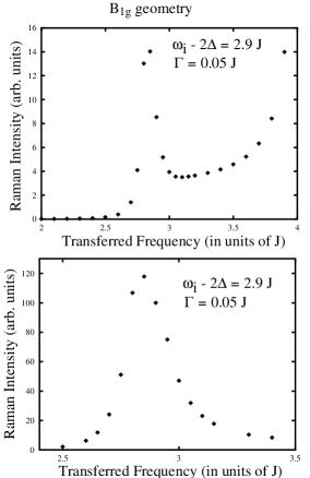
FIG. 6.: The Raman intensity as a function of transferred frequency $\Delta\omega$ for $\omega_{i}\approx\omega^{(1)}_{res}$ a) without and b) with a final state interaction.

The two-magnon lineshape obtained numerically is consistent with our analytical results in Sec. III B. There we attributed the asymmetry of the two-magnon profile to the branch cut in the Raman vertex which for $\omega_{i}=2\Delta+2.9J$ exists only for $\Delta\omega>2.8J$.
b) $\omega^{(1)}_{res}<\omega_{i}<\omega^{(2)}_{res}$
The form of the Raman profile changes quite strongly as one moves from $\omega^{(1)}_{res}$ to intermediate incident frequencies. In Fig. 7 we present, as an example, the Raman intensity including a final state interaction for $\omega_{i}=2\Delta+6.0J$. A comparison with Figs. 6 shows that the anisotropy of the intensity is now much stronger. This result is quite expected since in this range of incident frequencies, the Raman vertex resonates at transferred frequencies above the two-magnon peak. In particular, for $\omega_{i}=2\Delta+6J$, the triple resonance occurs near the maximum transferred frequency $\Delta\omega=4J$ (see Fig. 3).

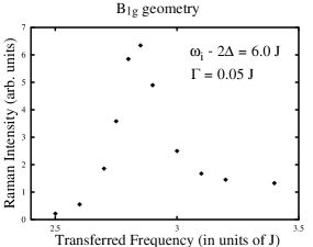
FIG. 7.: The Raman intensity as a function of transferred frequency $\Delta\omega$ for $\omega_{i}-2\Delta=6.0J$ in the interacting case.

The two-magnon profile for intermediate frequencies within the triple resonance theory was earlier obtained by Schönfeld et al.. Our results are in full agreement with theirs.
c) $\omega_{i}\approx\omega^{(2)}_{res}$
The results for the intensity with and without final state interaction are presented in Fig. 8b,a, respectively. The intensity without a final state interaction again exhibits an unphysical divergence at the maximum transferred frequency $\Delta\omega=4J$ which disappears when one includes a magnon-magnon scattering. Near $\omega^{(2)}_{res}$, however, this divergence is confined to a very narrow region near $4J$.
Furthermore, we obtain that in both figures the peak at around $\Delta\omega=2.8J$ is almost symmetric. This is also consistent with our analytical results in Sec. III A.
In addition to the peak at $\Delta\omega=2.8J$, both intensities also possess a slight maximum around $3.3J$ which probably originates from subleading, branch cut terms in the intensity.

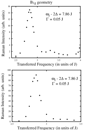
FIG. 8.: The Raman intensity as a function of transferred frequency $\Delta\omega$ for $\omega_{i}=\omega_{res}^{(2)}$, a) without and b) with a final state interaction.

The evolution of the Raman profile with increasing $\omega_{i}$ from slightly asymmetric form around $\omega_{res}^{(1)}$ to a pronounced shoulder-like behavior for intermediate frequencies, to a symmetric form close to $\omega_{res}^{(2)}$ is fully consistent with the experimental results on $Sr_{2}CuO_{2}Cl_{2}$ and $YBa_{2}Cu_{3}O_{6.1}$. We consider this agreement with the data as yet another evidence that the triple resonance diagram dominates the scattering process in the resonance regime.

B Two-magnon peak height

We now discuss the TMPH as a function of $\omega_{i}$. For the calculation of the TMPH, we fix the transferred frequency at a value which corresponds to the maximum of the two magnon profile (which, depending on $\omega_{i}$, occurs between $\Delta\omega=2.8J$ and $\Delta\omega=2.9J$) and plot the intensity of the maximum as a function of $\omega_{i}$. We present the results in Fig. 9 for two different values of the fermionic damping $\Gamma$. In both cases we clearly observe two maxima at $\omega^{(1)}_{res}\approx 2.9J$ and $\omega^{(2)}_{res}\approx 7.9J$. The positions of these maxima are in good agreement with the analytical predictions and the experimental data. The form of the TMPH near $\omega^{(1)}_{res}$ is clearly asymmetric: the intensity drops faster above the peak than below. This form agrees with our analytical results. For intermediate incident frequencies ($4.0J<(\omega_{i}-2\Delta)<7.5J$) the TMPH remains basically constant and, in addition, is practically $\Gamma$-independent. This behavior, we believe, results from the fact that in this frequency range the triple resonance occurs at $\Delta\omega=4J$ which is too far away from the two-magnon peak to influence its height.
Upon increasing $\Gamma$, we find that the TMPH around $\omega_{res}^{(2)}$ drops much more rapidly than around $\omega_{res}^{(1)}$. This is fully consistent with our analytical result that the divergence in the Raman vertex, which is only cut by the fermionic damping, is present only near $\omega_{res}^{(2)}$ while the maximum near $\omega_{res}^{(1)}$ is just an enhancement which does not crucially depend on the damping.

We also obtained two results which are not fully consistent with the experimental data. The first one is the ratio of intensities at the two maxima. We found that while the divergence in $M_{R}$ exists only near $\omega_{res}^{(2)}$, the non-divergent terms are much stronger around $\omega_{res}^{(1)}$. As a result, the ratio of intensities $I(\omega_{res}^{(1)})/I(\omega_{res}^{(2)})$ for $\Gamma=0.05J$ is $\approx 1$, while experimentally, this ratio is clearly smaller than one, though the actual number differs between $Sr_{2}CuO_{2}Cl_{2}$ and $YBa_{2}Cu_{3}O_{6.1}$.

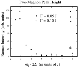
FIG. 9.: The TMPH as a function of incident frequency $\omega_{i}$.

The second discrepancy concerns the behavior of the TMPH in the vicinity of $\omega^{(2)}_{res}$. Analytically, we found that the TMPH should follow an inverse linear behavior at some distance from $\omega^{(2)}_{res}$ and an inverse cubic behavior in the immediate vicinity of $\omega^{(2)}_{res}$. To verify this result, we calculated the TMPH for several frequencies in the vicinity of $\omega^{(2)}_{res}$ and present the results in Fig. 10 (the dashed line in this figure is a guide to the eye). Within our numerical accuracy, we indeed found an inverse linear dependence which, however, only exists for a small region near $\omega^{(2)}_{res}$, namely for $0.1J<\omega^{(2)}_{res}-\omega_{i}<0.25J$. Experimentally, this region extends over a much wider frequency range of about $1eV$. Very close to $\omega^{(2)}_{res}$, the divergence is cut by the fermionic damping, and it is impossible to verify the predicted inverse cubic behavior.

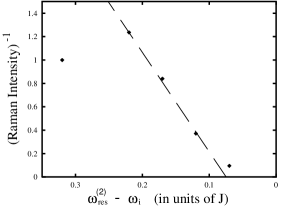
FIG. 10.: The inverse Raman intensity for $\Delta\omega=2.9J$ as a function of $\omega^{(2)}_{res}-\omega_{i}$.

We already mentioned that one of the reasons for the incorrect ratio of intensities $I(\omega_{res}^{(1)})/I(\omega_{res}^{(2)})$ lies in the oversimplified mean-field form of the fermionic dispersion, and, in particular, in the degeneracy along the boundary of the magnetic Brillouin zone. One would thus expect a better agreement with experiments if this degeneracy is lifted e.g., by the introduction of a finite next-nearest hopping $t^{\prime}$. We address this issue in the next subsection.

C Raman intensity for a nonzero $t^{\prime}$

In Sec. III C we found that a nonzero $t^{\prime}$ splits the triple resonance around $\omega^{(2)}_{res}$ into three double resonances one of which occur in the same region of the $(\omega_{i},\Delta\omega)$ plane as the triple resonance in the absence of $t^{\prime}$ while the other two occurs in different regions of the $(\omega_{i},\Delta\omega)$ plane. In Fig. 11 we plot the region of the $(\omega_{i},\Delta\omega)$ plane in which one of the remaining double resonances occurs. The form of the shaded area is similar to Fig. 3. We see that in the vicinity of $\omega^{(2)}_{res}$ the new resonant region reduces to a single line, just as the resonance for $t^{\prime}=0$. Near $\omega_{res}^{(1)}$ the situation is more complex since the different double resonances overlap.

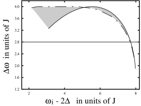
FIG. 11.: The shaded area describes the region of the $(\omega_{i},\Delta\omega)$ plane in which a double resonance occurs for $\omega_{i}-2E_{k}=0$ and $\omega_{i}-{\Delta\omega\over 2}+E_{k-q}^{v}-E_{k}^{c}=0$. The solid line corresponds o $q_{x}=q_{y}$ and the dashed line to $q_{x}=0$.

In Fig. 12 we present the result for the TMPH for $t^{\prime}/t=-0.16$. A comparison with Fig. 9 for the TMPH at $t^{\prime}=0$ shows that a finite $t^{\prime}$ reduces the TMPH at both resonant frequencies $\omega^{(1,2)}_{res}$. This reduction is fully consistent with our analytical calculations since now only two terms in the denominator of the Raman vertex vanish simultaneously while the third scales as $O(t^{\prime}/t)$. The reduction, however, is not uniform, and the TMPH around the high frequency resonance decreases much more rapidly than the one around the low-frequency resonance. Most probably, the increase of the ratio is caused by two effects. First, the regions of double resonance overlap around $\omega^{(1)}_{res}$, but not around $\omega^{(2)}_{res}$. Second, a nonzero $t^{\prime}$ also affects the interaction vertex $V_{lf}$ between light and fermions and reduces it much more strongly around $\omega_{res}^{(2)}$ than around $\omega_{res}^{(1)}$. To see this, we recall that in the mean-field approximation we have $V_{lf}=(\partial\epsilon_{k}/\partial\vec{k})\ \hat{e}_{i,f}$ with $\epsilon_{k}=-2t(\cos k_{x}+\cos k_{y})+4|t^{\prime}|\cos k_{x}\cos k_{y}$. Near $\omega^{(2)}_{res}$, the dominant contribution to the Raman vertex comes from fermions near the bottom of the band (${\bf k}\approx 0$) in which case the vertex between light and fermions is reduced by a factor of $(1-2|t^{\prime}|/t)$. In contrast, the resonance near $\omega^{(1)}_{res}$ is dominated by fermions near the top of the valence band ($k=(\pm\pi/2,\pm\pi/2))$ in which case the effect of $t^{\prime}$ is negligible.

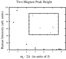
FIG. 12.: The TMPH as a function of the incident frequency $\omega_{i}$ for $t^{\prime}/J=-0.3$ and $\Gamma=0.05J$. The inset shows that despite the strong reduction one can still observe a maximum around $\omega_{res}^{(2)}$.

We see therefore that the inclusion of a finite $t^{\prime}$ actually worsens the agreement with the experiments since the ratio of intensities increases. In the next subsection we will consider whether vertex corrections can possibly reverse the effects of $t^{\prime}$ and restore the correct quantitative behavior of the TMPH.

D Vertex Corrections

There are several vertices in the diagram for the Raman matrix element, each of which is renormalized by vertex corrections which are generally not small at large $U$. The calculation of all vertex corrections is beyond our computational abilities and in this section we will therefore focus on the corrections to the vertex between light and fermionic quasiparticles, $V_{lf}$. Some evidence that the vertex between light and fermions near $\omega^{(2)}_{res}$ is larger than in the mean-field theory comes from the measurements of the optical conductivity in $Gd_{2}CuO_{4}$, $Pr_{2}CuO_{4}$ and $YBa_{2}Cu_{3}O_{6}$ [22]. These experiments have demonstrated that the measured conductivity is larger than the one calculated with the mean-field form for $V_{lf}$ even though it basically follows the same frequency dependence. We will study the vertex corrections to $V_{lf}$ semi-phenomenologically and our goal will be to illustrate how they can, in principle, reverse the effects of $t^{\prime}$.
The lowest order correction to $V_{lf}$ in a formal perturbative expansion in $1/S$ is presented in Fig. 13. A simple analysis shows that the relative vertex correction scales as $U/JS$, i.e., it is small only in the limit of a very large spin. For realistic $S$, however, we have $U/JS\gg 1$, and the corrections to $V_{lf}$ are large. This clearly implies that one should sum up an infinite series of corrections to obtain the proper renormalization of the vertex between light and fermions.

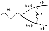
FIG. 13.: The lowest order vertex corrections to the light-quasiparticle interaction. The solid and dashed lines represent the conduction and valence band quasiparticles, respectively. The internal wavy line describes the exchange of a magnon.

We will not do this but rather model the effect of the vertex corrections phenomenologically by introducing an effective vertex in the form

$$V^{eff}_{lf}(k)=\Big{(}\displaystyle{\partial\epsilon_{k}\over\partial\vec{k}}\hat{e}_{i,f}\Big{)}\Big{(}1+\alpha\;\nu_{k}^{2}\Big{)}$$ (68)

with $\alpha$ as a parameter. The effective vertex in Eq.(68) still possesses the same symmetry as the bare vertex $V_{lf}(k)$ and therefore still vanishes at the bottom of the band. However, the slope of $V^{eff}_{lf}(k)$ around ${\bf k}=0$ can now be quite different from the mean-field result.

We computed the TMPH with the effective vertex using various values of $\alpha$. The result for $\alpha=0.5$ is presented in Fig. 14.

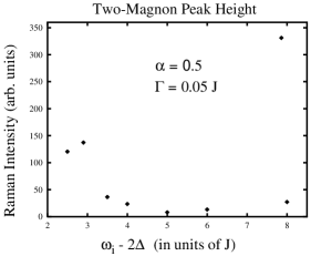
FIG. 14.: The TMPH for $\Gamma=0.05J$ and $\alpha=0.5$.

A comparison with Fig. 9 shows that the effect of the vertex correction is rather strong; the ratio $I(\omega^{(1)}_{res})/I(\omega^{(2)}_{res})$ is decreased by a factor of about $2.5$. In addition, we also observe a relative increase of the TMPH for intermediate $4.5J\leq(\omega_{i}-2\Delta)\leq 5.5J$. This last effect leads to an extension of the region in which the Raman intensity possesses an inverse linear behavior.

The decrease of the ratio of the intensities and the extension of the frequency range of the inverse linear behavior are both in agreement with the experimental results [20]. We therefore see that by adjusting the vertex corrections to $V_{lf}(k)$ without violating the symmetry requirements of the model, one can, in principle, not only obtain good qualitative, but also quantitative agreement with the experimental data. The question is, however, whether, e.g., $\alpha=0.5$ which we used in Fig. 14 can be obtained in a microscopic calculation. These studies are clearly called for.

V Discussion

We first summarize our results. The intent of this paper was to study the full Raman intensity in the resonant regime by simultaneously considering the effects of the triple resonance in the Raman vertex and the final state magnon-magnon interaction. We derived an explicit expression for the full Raman intensity in the resonant regime as a function of both, transferred frequency $\Delta\omega$ and incoming frequency $\omega_{i}$. We obtained analytically and numerically the two-magnon Raman profile as a function of the transferred photon frequency $\Delta\omega$ and the dependence of the two-magnon peak height on the incident photon frequency $\omega_{i}$. We found that the resonant behavior of the Raman vertex survives the inclusion of a magnon-magnon interaction and obtained two maxima in the peak height at $\omega_{res}^{(1)}\approx 2\Delta+2.9J$ and at $\omega_{res}^{(2)}\approx 2\Delta+7.9J$. The position of the two maxima are the same as in the semi-phenomenological approach by CF which considered the triple resonance enhancement and final state interaction independent of each other. We first studied in detail the two-magnon profile at various incident frequencies. We found that the two-magnon peak is slightly asymmetric near $\omega_{res}^{(1)}$ with larger intensity at higher frequencies. As the incident frequency increases, the asymmetry becomes stronger, and the two-magnon profile acquires a shoulder-like feature above the peak. This is consistent with earlier results [25]. For frequencies around $\omega_{res}^{(2)}$, however, we found that the anisotropy disappears, and the Raman profile acquires almost the same form as in the nonresonance, LF regime.

We then proceeded to a more detailed study of the two-magnon peak height. We verified that the inverse linear behavior of the Raman intensity near $\omega^{(2)}_{res}$ survives the effect of the final state interaction. Furthermore, we considered the behavior of the Raman vertex near $\omega_{res}^{(1)}$. We found in our analytical considerations for which we assumed an isotropic dispersion near the top of the band that the divergence is almost completely suppressed. However, the Raman vertex contains a branch cut which gives rise to an enhancement of the intensity in some range of frequencies $\omega_{i}\leq\omega_{res}^{(1)}$ which terminates only slightly below $\omega_{res}^{(1)}$. In our numerical calculations, for which we considered a mean-field form of the dispersion, we obtained a weak singularity at $\omega_{res}^{(1)}$ but also a strong enhancement of the Raman intensity for $\omega_{i}$ slightly smaller than $\omega_{res}^{(1)}$. This last enhancement is virtually independent of the damping.

We found that the ratio of the Raman intensities $I(\omega^{(1)}_{res})/I(\omega^{(2)}_{res})$ is already rather large for small damping, contrary to the assertion by CF. A much smaller ratio is needed for a quantitative agreement with the experimental data. We attribute the large ratio to an unexpectedly strong enhancement of the two-magnon peak near $\omega^{(1)}_{res}$ due to a branch-cut anomaly in the Raman vertex.

We further studied how the the triple resonance is modified by a next-nearest hopping term $t^{\prime}$. Around $\omega_{res}^{(2)}$, we found that the triple resonance is split into three double resonances, but the linear divergence of the Raman intensity near $\omega_{res}^{(2)}$ is not changed. This splitting, however, reduces the intensity around $\omega_{res}^{(2)}$ relative to the intensity around $\omega_{res}^{(1)}$ where the effect of a finite $t^{\prime}$ is rather weak. As a result, the ratio of the intensities $I(\omega^{(1)}_{res})/I(\omega^{(2)}_{res})$ increases.

Finally, we have demonstrated that the ratio of the intensities at the two resonance values of $\omega_{i}$ is sensitive to the actual form of the vertex between light and fermions. We have shown that the corrections to the mean-field vertex are large and modeled their effect by introducing an extra factor $(1+\alpha\nu_{k}^{2})$ into the vertex. We considered $\alpha$ as an adjustable parameter and showed that the ratio of the intensities can be substantially reduced already for moderate values of $\alpha$.

We now discuss our results in the context of the key experimental features that we listed in the introduction as being in disagreement with the LF theory:
1) Changing lineshape with $\omega_{i}$
Our results for the evolution of the Raman profile with $\omega_{i}$ is in complete agreement with the experimental results by Blumberg et al. [20] on $YBa_{2}Cu_{3}O_{6.1}$. For $Sr_{2}CuO_{2}Cl_{2}$, the highest experimentally accessible frequency is smaller than $\omega_{res}^{(2)}$ and we therefore do not know whether the Raman profile eventually becomes symmetric near $\omega_{res}^{(2)}$. For intermediate $\omega_{i}$, however, our results agree with the experimental data.

An issue which we have not addressed in our approach is the actual rather than relative width of the two-magnon peak. Experimentally, it is much broader than in our model. Previous studies by Weber and Ford [37], however, have shown that the broadening may be due to a magnon damping. They demonstrated that a small damping due to, e.g., an interaction with phonons already gives rise to a considerable broadening of the two-magnon peak. This result has also been obtained in numerical studies [38].

Another reason for the broadening of the Raman lineshape is the fermionic damping $\Gamma$. Incidentally, this damping may also account for the experimentally observed additional broadening of the TMPH around $\omega_{res}^{(2)}$ since in this frequency range, the dominant contribution to $M_{R}$ comes from fermions with ${\bf k}\approx 0$ which exhibit the largest damping [20].

2) The TMPH as a function of $\omega_{i}$
The two key experimental results for the TMPH, we remind, are the presence of two maxima in the TMPH, of which the higher frequency maximum is stronger in all compounds, and an inverse linear behavior of the Raman intensity near the upper resonance frequency $\omega^{(2)}_{res}$. In our analytical and numerical calculations we found the two maxima in the TMPH whose positions fully agree with the experimental data. In addition we found that the low-frequency maximum in the TMPH is anisotropic with a higher intensity at lower frequencies which is also consistent with the experimental results.

Our numerical data, however, differ quantitatively from the experimental results in that the ratio $I(\omega_{res}^{(1)})/I(\omega_{res}^{(2)})$ is too large. On the basis of our analytical results we would expect the opposite behavior since we found that the actual resonance in the Raman intensity (i.e. a divergence in the absence of a fermionic damping) exists only near $\omega^{(2)}_{res}$ while the peak near $\omega^{(1)}_{res}$ is just the enhancement due to nonsingular terms in the Raman vertex. It turns out however that these nonsingular terms are anomalously large. Naively, one would expect that the inclusion of a next-nearest neighbor hopping $t^{\prime}$ would lead to an improved agreement of the ratio with the experimental data. In contrast, we found that a finite $t^{\prime}$ suppresses the high-frequency resonance even further. On the other hand, we have demonstrated that the inclusion of the corrections to the interaction between light and fermions may substantially increase the vertex near $\omega^{(2)}_{res}$ compared to the vertex near $\omega^{(1)}_{res}$. This eventually yields a much better ratio of $I(\omega_{res}^{(1)})/I(\omega_{res}^{(2)})$ which can be made fully consistent with the experimental data by adjusting the magnitude of the vertex correction.

Our analytical and numerical computations also reproduced the inverse linear behavior of the Raman intensity, which was observed in $YBa_{2}Cu_{3}O_{6.1}$ [20] and $PrBa_{2}Cu_{3}O_{7}$ [21] and, to a certain extent, also in $Sr_{2}CuO_{2}Cl_{2}$. However, we also found that the range of $\omega_{i}$ in which this behavior was observed experimentally is much larger than in our analysis. The inclusion of the vertex corrections improves the agreement with the data but does not make it perfect. This issue requires further study.

In conclusion we have provided a detailed study of Raman scattering in the resonant regime. We confirmed that the key experimental features of magnetic Raman scattering can be explained qualitatively, and to some extent quantitatively within the triple resonance theory. We believe that the remaining quantitative discrepancies are due to insufficient knowledge of the quasi-particle energy dispersion, lifetime effects and the form of the vertex function between light and fermions.

A final remark. We discussed in Sec. IV A that for intermediate incident frequencies, $\omega^{(1)}_{res}<\omega<\omega^{(2)}_{res}$, the triple resonance occurs relatively far from the two-magnon peak and, to first approximation, does not influence the two-magnon lineshape. In other words, in calculating the two-magnon lineshape, one can, with reasonable accuracy, set the denominator in the triple resonance diagram to a constant and compute the Raman vertex in the same way as in the LF theory. It turns out that this procedure yields good agreement with the data not only in $B_{1g}$ but also in other scattering geometries. To demonstrate this, we present in Fig. 15 the results for the intensity in four different scattering geometries. These results have to be compared with the experimental data for $Sr_{2}CuO_{2}Cl_{2}$ and $YBa_{2}Cu_{3}O_{6.1}$ [39]. which we reproduce in Fig. 16. Since $J\sim 1000cm^{-1}$, the comparison with Fig. 15 is valid only for $\Delta\omega\leq 4000cm^{-1}$. A finite scattering intensity at larger $\Delta\omega$ is probably due to multi-magnon scattering.

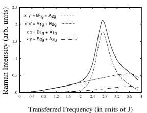
FIG. 15.: The Raman intensity as a function of transferred frequency $\Delta\omega$ for constant denominator.

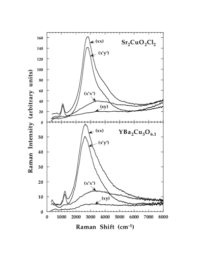
FIG. 16.: Two-magnon Raman scattering spectra from Sr₂CuO₂Cl₂ and YBa₂Cu₃O_6.1 at room temperature in different scattering geometries. Courtesy of the authors of Ref. [39]. The labels indicate: $xx$ ($B_{1g}+A_{1g}$), $x^{\prime}y^{\prime}$ ($B_{1g}+A_{2g}$), $x^{\prime}x^{\prime}$ ($A_{1g}+B_{2g}$) and $xy$ ($B_{2g}+A_{2g}$) The excitation energy is $2.73$ eV, which is about $0.4$ eV below $\omega_{res}^{(2)}$.

We consider the agreement between the two figures as rather good and view it as an another piece of evidence in favor of the triple resonance theory.

Acknowledgments

It is our pleasure to thank J. Betouras, G. Blumberg, D. Frenkel, R. Joynt and M.V. Klein for helpful conversations. The research was supported by NSF-DMR 9629839. A.C. is an A.P. Sloan fellow.

A The Raman intensity with magnon-magnon interaction

In this appendix we present the formulae for the numerical computation of the full Raman intensity. Our starting point is the Golden Rule formula, Eq.(1)

$$R(\omega_{i},\Delta\omega)\propto\int{d^{2}q\over 4\pi^{2}}|M^{tot}_{R}(\omega_{i},\Delta\omega,q)|^{2}\delta(\Delta\omega-2\omega_{q})$$ (A1)

where $M^{tot}_{R}$ is diagrammatically presented in Fig.1b. The Golden Rule formula for the intensity corresponds to the diagram in Fig. 1a in which the intermediate magnons are on the mass shell.
The analytical expression for $M_{R}^{tot}$ has the form

$$M^{tot}_{R}=M_{R}+{\bar{M}_{R}\ \tilde{\nu}_{q}\over 1+I/4S}$$ (A2)

where $I$ is given in Eq.(7), and $M_{R}$ and $\bar{M}_{R}$ are given by Eqs.(10) and (14) for $t^{\prime}=0$ and by Eqs.(53) and (56) for $t^{\prime}\neq 0$, respectively.
Note that we use the full form of $M_{R}$ and do not project it on $\tilde{\nu}_{q}$ as was done in Ref.[25]. Our numerical computations show that especially for small $\Gamma$, the $B_{1g}$ component of $M_{R}$ has a more complex dependence on the magnon momentum than just ${\tilde{\nu}}_{q}$.

REFERENCES

- [1] P.W. Anderson, Science 235, 1196 (1987).
- [2] P.W. Anderson and J.R. Schrieffer, Physics Today 44(6), 54 (1991), and references therein.
- [3] See the discussion by P.W. Anderson, D. Pines, and D.J. Scalapino in Physics Today 47(2), 9 (1994); also a column in Science 261, 294 (1993).
- [4] D. Pines, in High Temperature Superconductivity and the C60 Family, ed. H.C. Ren, p. 1 (Gordon and Breach, 1995); P. Monthoux and D. Pines, Phys. Rev. B 47, 6069 (1993); Phys. Rev. B 50, 16015 (1994); Phys. Rev. B 49, 4261 (1994).
- [5] D.J. Scalapino, E. Loh, and J.E. Hirsch, Phys. Rev. B, 34, 8190 (1986); D.J. Scalapino, Phys. Rep. 250, 329 (1995) and references therein.
- [6] R. Merlin, Journal de Physique (Paris), Colloque C5, 41, C5-233 (1980).
- [7] M.G. Cottam and D.L. Lockwood, Light Scattering in Magnetic Solids (Wiley, New York, 1986).
- [8] R.R.P. Singh, Comments Cond. Mat. Phys. 15, 241 (1991).
- [9] A.P. Kampf and W. Brenig, Z. Phys. B 89, 313 (1991).
- [10] W. Hayes and R. Loudon, Scattering of Light by Crystals (Wiley-Interscience, New York, 1978) and references therein.
- [11] C.M. Canali and S.M. Girvin, Phys. Rev. B 45, 7121 (1992).
- [12] K.B. Lyons, P.A. Fleury, L.T. Schneemeyer, and J.V. Waszczak, Phys. Rev. Lett. 60, 732 (1988).
- [13] I. Tomeno, M. Yoshida, K. Ikeda, K. Tai, K. Takamuku, N. Koshizuka, S. Tanaka, K. Oka, and H. Unoki, Phys. Rev. B 43, 3009 (1991).
- [14] G. Blumberg, R. Liu, M.V. Klein, W.C. Lee, D.M. Ginsberg, C. Gu, B.W. Veal, and B. Dabrowski, Phys. Rev. B 49, 13296 (1994).
- [15] P.A. Fleury and R. Loudon, Phy. Rev. 166, 514, (1968).
- [16] K.B. Lyons, P.A. Fleury, J.P. Remeika, A,S. Cooper, and T.J. Negran, Phys. Rev. B 37, 2353 (1988).
- [17] P.E. Sulewsky, P.A. Fleury, K.B. Lyons, S.-W. Cheong, and Z. Fisk, Phys. Rev. B 41, 225 (1990).
- [18] S.M. Hayden, G. Aeppli, H. Mook, D. Rytz, M.F. Hundley, and Z. Fisk, Phys. Rev. Lett. 67, 3622 (1991).
- [19] T. Imai, C.P. Slichter, K. Yoshimura, and K. Kosuge, Phys. Rev. Lett 70, 1002 (1993).
- [20] G. Blumberg. P. Abbamonte, M.V. Klein, W.C. Lee, D.M. Ginsberg, L.L. Miller, and A. Zibold, Phys. Rev. B 53, R11930 (1996).
- [21] M. Rübhausen, N. Dieckmann, A. Bock, U. Merkt, W. Widder, and H.F. Braun, Phys. Rev. B 53, 8619 (1996).
- [22] R. Liu, M.V. Klein, D. Salamon, S.L. Cooper, W.C. Lee, S.W. Cheong, and D.M. Ginsberg, J. Phys. Chem. Solids 54, 1347 (1993); S.L. Cooper et al., Phys. Rev. B 47, 8233 (1993).
- [23] B. Shastry and B. Shraiman, Phys. Rev. B 65, 1068 (1990); Int. J. Mod. Phys. B 5, 365 (1991).
- [24] A.V. Chubukov and D.M. Frenkel, Phys. Rev. Lett. 74, 3057 (1995); Phys. Rev B 52, 9760 (1995).
- [25] F. Schönfeld, A.P. Kampf, and E. Müller-Hartmann, Z. Physik B 102, 25 (1997).
- [26] B.O. Wells et al, Phys. Rev. Lett. 74, 964 (1995).
- [27] S. LaRosa et al., Phys. Rev. B, to appear.
- [28] R.W. Davis, S.R. Chinn, and H.J. Zeiger, Phys. Rev. B 4, 992, (1971).
- [29] A.V. Chubukov and K.A. Musaelian, Phys. Rev. B 50, 6238 (1994).
- [30] A. Singh. Phys. Rev. B 43, 3617 (1991).
- [31] J. Altmann, W. Brenig, A.P. Kampf, and E. Müller-Hartmann, Phys. Rev. B 52, 7395 (1995).
- [32] R.B. Laughlin, preprint cond-mat 9608005.
- [33] D. Duffy and A. Moreo, Phys. Rev. B 52, 15607 (1995).
- [34] R. Preuss, W. Hanke, and W. von der Linden, Phys. Rev. Lett. 75, 1344 (1995).
- [35] E. Dagotto, Rev. Mod. Phys. 66, 763 (1994).
- [36] D.K. Morr and A.V. Chubukov, in preparation.
- [37] W.H. Weber and G.W. Ford, Phys. Rev. B 40, 6890 (1989).
- [38] F. Nori, R. Merlin, S. Haas, A.W. Sandvik, and E. Dagotto, Phys. Rev. Lett. 75, 553 (1995).
- [39] G. Blumberg, P. Abbamonte, and M.V. Klein, SPIE-Proceedings 2696, 205 (1996).