The Fermi Liquid as a Renormalization Group Fixed Point: the Role of Interference in the Landau Channel

Abstract

We apply the finite-temperature renormalization-group (RG) to a model based on an effective action with a short-range repulsive interaction and a rotation invariant Fermi surface. The basic quantities of Fermi liquid theory, the Landau function and the scattering vertex, are calculated as fixed points of the RG flow in terms of the effective action’s interaction function. The classic derivations of Fermi liquid theory, which apply the Bethe-Salpeter equation and amount to summing direct particle-hole ladder diagrams, neglect the zero-angle singularity in the exchange particle-hole loop. As a consequence, the antisymmetry of the forward scattering vertex is not guaranteed and the amplitude sum rule must be imposed by hand on the components of the Landau function. We show that the strong interference of the direct and exchange processes of particle-hole scattering near zero angle invalidates the ladder approximation in this region, resulting in temperature-dependent narrow-angle anomalies in the Landau function and scattering vertex. In this RG approach the Pauli principle is automatically satisfied. The consequences of the RG corrections on Fermi liquid theory are discussed. In particular, we show that the amplitude sum rule is not valid.

I Introduction

In 1956-1957 L.D. Landau formulated his theory of Fermi liquids.[1] The original phenomenological formulation of this theory is based on an expansion near the ground state of the energy functional in terms of variations of the distribution function (bosonic variables). Later, Pomeranchuk derived the thermodynamic stability conditions for this functional.[2] Much effort has been dedicated, including by Landau himself,[3] to vindicate some intuitive assumptions of Landau and elucidate the foundations of the phenomenological Fermi Liquid Theory (FLT). The field-theoretic interpretation of the Landau FLT has reformulated the key notions and basic results of the phenomenological theory entirely in terms of the fermionic Green functions technique.[3, 4, 5, 6] The demonstration of the equivalence of the field-theoretic results obtained from the solution of the Bethe-Salpeter equation with the results obtained from the functional expansion and from the Boltzmann transport equation describing the collective modes, has become a textbook topic.[5, 6, 7, 8, 9] The field-theoretic approach provided not only a solid basis to phenomenology, but also a potentially efficient method to calculate the phenomenological parameters of FLT from first principles.

Current interest in non-Fermi Liquids in $d>1$ inspired a new wave of efforts aimed at clarifying the foundations of the Landau FLT and the mechanisms of its breakdown. Let us mention only two approaches, which can be seen as sophisticated modern counterparts of the two classic formulations of the Landau FLT. A bosonized treatment of Fermi liquids has recently been developed[10] in the framework of Haldane’s formulation of higher-dimensional bosonization.[11] At about the same time, the Renormalization Group (RG) technique has been applied to interacting fermions in $d>1$ with models based on fermionic field effective actions (see Refs [12, 13, 14, 15, 16, 17, 18, 19, 20] and references therein). It both approaches it has been established, for models with reasonable fermion-fermion effective interactions, that the Fermi liquid phase is stable, whereas adding gauge-field interactions may drive the system towards a Non-Fermi-Liquid regime, or may result in a Marginal Fermi Liquid phase, like for composite fermions at the half-filled Landau level.

The RG analysis of FLT presented here and in our previous work,[19] like other such analyses already published, starts from a low-energy effective action with a marginal (in the RG sense) short-range interaction. However, contrary to other works on the subject, our finite-temperature RG approach revealed that, in the Landau channel of nearly forward scattering quasiparticles, the effective interaction flows with successive mode eliminations towards the Fermi surface, even in the absence of singular or gauge interactions. In other words, the action’s interaction (coupling function) does not stay as a purely marginal under the RG transformation, since its $\beta$-function is not identically zero. From the RG flow equations the standard FLT results have been recovered.[19]

It was also pointed out, and elaborated later in more detail by one of us together with N. Dupuis in Ref.[20], that the bare interaction function of the low-energy fermion effective action cannot be identified with the Landau interaction function. The latter, along with other observable parameters of a Fermi liquid, should be calculated as a fixed point of the RG equations.[20] Let us briefly give two arguments for this. First, identifying the Landau function with the effective action’s bare interaction is inconsistent with other standard FLT results, due to the role of Fermi statistics. Indeed, in a stable Fermi liquid, the well-known relationship between components of the scattering amplitude ($\Gamma_{l}$) and of the Landau interaction function ($F_{l}$), i.e., $\Gamma_{l}=F_{l}/(1+F_{l})$, cannot satisfy the Pauli principle for the amplitude (the amplitude sum rule) if $F$ has the symmetry properties of the action’s bare interaction. (For the explanation of this point see Sect. V below). Second, identifying the Landau function with the bare interaction is inconsistent with the low-energy effective action method itself, in the way it is applied to condensed matter problems. Namely, at the starting point of the analysis, the bare parameters of the effective action, including the interaction, are regular functions of their variables.[14, 15] It is known, however, that this is not the case even for parameters of a normal Fermi liquid. For instance, the scattering amplitude and the Landau function are two distinct limits of the four-point vertex in the Landau channel when energy-momentum transfer goes to zero. The non-analyticity of the forward scattering vertex appears in its dependence both on the small energy-momentum transfer and, due to the antisymmetry (crossing symmetry), on the small angles between incoming (outgoing) particles lying near the Fermi surface. This contradiction becomes flagrant if one couples the fermionic action with gauge fields since, as shown by other methods,[21] the Landau function for the marginal Fermi Liquid of composite fermions at the half-filled Landau level develops a delta-function singularity in the forward direction ($\theta=0$). Such behavior of the Landau function is related to the divergence of the quasiparticle’s effective mass, according to the theory of Halperin, Lee and Read for the half-filled Landau level[22] (see also Ref[23]). So, coming back to our arguments, the Landau function cannot be a regular interaction in the effective action at the starting point of the RG analysis.

The aim of the present study is twofold. Once the classic FLT results have been recovered by the RG approach,[19] the latter would loose its appeal if it did not provide a constructive method for calculating the Fermi liquid’s parameters. This is especially important goal in the long-term prospective of applying this powerful method to more complex strongly correlated fermion systems. In this work we explicitly derive the Landau function and the forward scattering vertex from the short-range effective bare interaction. We do it in the one-loop RG approximation which takes into account contributions of the direct ($ZS$) and exchange $(ZS^{\prime})$ graphs. This enables us to reveal singular features of the Landau function and scattering vertex in the forward direction ($\theta=0$).

An equally important goal of this work is to resolve the old problem of FLT with the Pauli principle. In its treatment of FLT, the field-theoretic approach encountered a very subtle problem caused by Fermi statistics of one-particle excitations and by the necessity to provide both stability for the Fermi liquid and a solution for the two-particle vertex that meets the Pauli principle.[24, 7] The problem was “settled” by imposing the amplitude sum rule on the components of the Landau quasiparticle’s interaction function. The phenomenological FLT is spared from this problem partially by the way it is formulated, partially because it says nothing about the quasiparticle scattering amplitudes. (A detailed discussion of this problem, which lies at the heart of the present study, is postponed until Sec.V, where it will be put in contact with the present RG approach.) The same problem arose in our previous work[19] in the form of a “naturalness problem”[14] of the effective action: the effective action had to be “fine tuned” in order for the scattering amplitude to meet the Pauli principle. We will show that if quantum interference of the direct and exchange processes is taken into account, this problem is eliminated in a natural manner.

The paper is organized as follows. Sections II and III are introductory: we define the effective action of the model and the coupling functions (the bare interaction) and vertices to be calculated in the Landau interaction channel. In Section IV, which is rather technical, the one-loop RG equations for the two-dimensional case are derived. Section V explains some of the weak points of the standard FLT results and argues for their partial revision. In Section VI we give a numerical and approximate analytical solution of the coupled RG equations for spinless fermions. In Section VII we present and discuss our results for the Landau function and the scattering vertex calculated at different temperatures. In Section VIII we relate this study to the standard treatment of Fermi liquid Theory. The consequences of the RG corrections on FLT results are discussed.

II The Model

We apply the Wilson-Kadanoff renormalization scheme in the framework developed earlier for a model with $SU(N)$-invariant short-range effective interaction and rotation invariant Fermi surface in spatial dimensions $d\leq 3$ at finite temperature.[19] In order to make the discussion as clear as possible, we concentrate in this work on $2D$ spinless ($N=1$) fermions. This simple model has nevertheless all the necessary qualities to illustrate our key points and to demonstrate the new features brought by the RG analysis of a Fermi liquid. In this case the RG equations take their simplest form, since only the antisymmetric momentum-frequency dependent parts of the interaction and vertices are present (they were labeled by A in Ref.[19]).

The partition function in terms of Grassmann variables is given by the path integral

$$Z=\int{\cal D}\bar{\psi}{\cal D}\psi~{}e^{S_{0}+S_{\rm int}}$$ (1)

wherein the free part of the effective action[14, 15, 16] is

$$S_{0}=\int_{({\bf 1})}\bar{\psi}({\bf 1})\left[i\omega_{1}+\mu-\epsilon({\bf K}_{1})\right]\psi({\bf 1})~{}.$$ (2)

We introduced the following notation:

$$\int_{({\bf i})}~{}~{}\equiv~{}~{}{1\over\beta}\int{d{\bf K}_{i}\over(2\pi)^{2}}\sum_{\omega_{i}}$$ (4)

$$({\bf i})~{}~{}\equiv~{}~{}({\bf K}_{i},\omega_{i}),$$ (5)

where $\beta$ is the inverse temperature, $\mu$ the chemical potential, $\omega_{i}$ the fermion Matsubara frequencies. We set $k_{B}=\hbar=1$. The interacting part of the action is

$$S_{\rm int}=-\frac{1}{4}\int_{({\bf 1},{\bf 2},{\bf 3},{\bf 4})}\bar{\psi}({\bf 1})\bar{\psi}({\bf 2})\psi({\bf 3})\psi({\bf 4})\Gamma^{\Lambda_{0}}({\bf 1},{\bf 2};{\bf 3},{\bf 4})\beta(2\pi)^{2}\delta({\bf 1}+{\bf 2}-{\bf 3}-{\bf 4})~{},$$ (6)

where $\delta(\cdots)$ stands for a Dirac delta function for the momenta and a Kronecker delta for the Matsubara frequencies. The function $\Gamma^{\Lambda_{0}}$ is antisymmetric under the exchange $({\bf 1}\leftrightarrow{\bf 2})$ and $({\bf 3}\leftrightarrow{\bf 4})$. The bare cutoff $\Lambda_{0}$ of the action is introduced such that each vector ${\bf K}_{i}$ in the effective action lies in a shell of thickness $2\Lambda_{0}$ around the Fermi surface. We denote this shell, i.e., the support of the effective action in the momentum space, as $C^{2}_{\Lambda_{0}}$. The Matsubara frequencies are allowed to run over all available values. We presume that the density of particles in the system is kept fixed.

The one-particle excitations are linearized near the Fermi surface, and therefore the bare one-particle Green’s function for the free part of action $S_{0}$ is:

$$G_{0}^{-1}({\bf K}_{1},\omega_{1})=i\omega_{1}+\mu-\epsilon({\bf K}_{1})\approx i\omega_{1}-v_{F}(K_{1}-K_{F})\equiv i\omega_{1}-v_{F}k_{1}~{}.$$ (7)

In the integration measure only the relevant part is kept:

$$\int d{\bf K}~{}=~{}\int_{-\Lambda_{0}}^{\Lambda_{0}}\int_{0}^{2\pi}{(K_{F}+k)}dkd\theta~{}\approx~{}K_{F}\int_{-\Lambda_{0}}^{\Lambda_{0}}\int_{0}^{2\pi}dkd\theta$$ (8)

The temperature $T$ is restricted by the condition

$$T\ll~{}v_{F}\Lambda_{0}~{}.$$ (9)

The relevant physical information can be obtained by studying interactions of particles scattering with small momentum and energy transfer (we call it the Landau channel), and those with nearly opposite incoming (outgoing) momenta (the BCS channel). Since we are interested in the repulsive case, we presume that stability conditions against Cooper pairing are fulfilled, and we concentrate on the Landau channel.

III Coupling functions and vertices in the Landau channel

Let us clarify the meaning of the quantities entering the effective action. Consider the vertex function $\Gamma({\bf 1},{\bf 2};{\bf 3},{\bf 4})$, constructed from the connected two-particle Green’s function ${G}_{2}^{c}({\bf 1},{\bf 2};{\bf 3},{\bf 4})=-\langle\psi({\bf 1})\psi({\bf 2})\bar{\psi}({\bf 3})\bar{\psi}({\bf 4})\rangle_{c}$ by amputation of the external legs. Here $\langle...\rangle$ means an average with the effective action (2,6) which contains only “slow” modes, lying in the support $C^{2}_{\Lambda_{0}}$. Once auxiliary source fields (with momenta inside the shell $C^{2}_{\Lambda_{0}}$) coupled to the action’s Grassmann fields $\{\psi$, $\bar{\psi}\}$ have been introduced, such connected $n$-particle Green’s functions can be defined as functional derivatives of the source-dependent generating functional.[25] At tree-level, $\Gamma({\bf 1},{\bf 2};{\bf 3},{\bf 4})|_{\rm tree}=\Gamma^{\Lambda_{0}}({\bf 1},{\bf 2};{\bf 3},{\bf 4})$. The bare vertex $\Gamma^{\Lambda_{0}}$ (in the sense of the effective action (2,6)) can be defined in the same fashion as $\Gamma$, with the difference that $\Gamma^{\Lambda_{0}}$ is the result of averaging over the “fast” modes (those outside $C^{2}_{\Lambda_{0}}$) with the microscopic action. Contrary to $\Gamma$, the vertex $\Gamma^{\Lambda_{0}}$ is not a physical observable, since it is not the result of an integration over all degrees of freedom.

Taking into account momentum and frequency conservation, we use the following notation for the nearly forward scattering vertex:

$$\Gamma({\bf 1},{\bf 2};{\bf 1}+{\cal Q},{\bf 2}-{\cal Q})\equiv\Gamma({\bf 1},{\bf 2};{\cal Q})~{},$$ (10)

with the transfer vector

$${\cal Q}={\bf 3}-{\bf 1}\equiv({\bf Q},\Omega)$$ (11)

such that $Q\ll K_{F}$ ($\Omega$ is a bosonic Matsubara frequency). We write the momentum ${\bf K}_{i}$ as ${\bf K}_{i}={\bf K}_{F}^{i}+{\bf k}_{i}$ where ${\bf K}_{F}^{i}$ lies on the Fermi surface and ${\bf k}_{i}$ ($|{\bf k}_{i}|\leq\Lambda_{0}$) is normal to the Fermi surface at the point ${\bf K}_{F}^{i}$.

In order to calculate physical quantities, we must perform an average with the effective action (2,6), i.e., we must integrate out the “slow” modes, which lie inside $C^{2}_{\Lambda_{0}}$, in the corresponding path integrals. This is done in Wilson’s RG approach by successively integrating the high-energy modes in $C^{2}_{\Lambda_{0}}$, i.e., by progressively reducing the momentum cutoff from $\Lambda_{0}$ to zero. We define a RG flow parameter $t$ such that the cutoff at an intermediate step is $\Lambda(t)=\Lambda_{0}e^{-t}$. Integrating over the modes located between the cutoffs $\Lambda(t)$ and $\Lambda(t+dt)$, a recursion relation (in the form of a differential equation) can be found for the various parameters of the action. This equation (or set of equations) is then solved from $t=0$ to $t\to\infty$ and this yields the fixed-point value of the parameters of the action. The physical quantities are then obtained from these parameters, e.g. by functional differentiation if they are source fields.

A considerable simplification of this problem comes from the scaling analysis of the low-energy effective action using the smallness of the scale $\Lambda/K_{F}$.[15] A tree-level analysis shows that the only part of the coupling function $\Gamma^{\Lambda}$ which is not irrelevant couples two incoming and two outgoing particles with the same pairs of momenta $({\bf K}_{F}^{1},{\bf K}_{F}^{2})$ lying on the Fermi surface. The dependence of the coupling function on ${\bf k}_{i}$ and on the frequencies $\omega_{i}$ is irrelevant and can be omitted. When the initial cutoff $\Lambda_{0}$ satisfies condition (9), we can unambiguously define a bare coupling function which depends only on the angle between the incoming (or outgoing) momenta. This bare coupling function is given by the vertex $\Gamma^{\Lambda_{0}}({\bf 1},{\bf 2};{\cal Q})$ in the zero transfer limit (${\cal Q}=0$) where the two external momenta are put on the Fermi surface and the external frequencies are $\omega_{\rm min}\equiv\pi T$ (the latter will be dropped from now on).

$$U({\bf K}_{F}^{1},{\bf K}_{F}^{2})\equiv\frac{1}{2}\nu_{F}\Gamma^{\Lambda_{0}}({\bf K}_{F}^{1},{\bf K}_{F}^{2};0)~{},$$ (12)

where $\nu_{F}=K_{F}/\pi v_{F}$ is the free density of states at the Fermi level. Each vector ${\bf K}_{F}^{i}$ may be specified by a plane polar angle $\theta_{i}$. The function $U$ is an even function of the relative angle $\theta_{12}$ between ${\bf K}_{F}^{1}$ and ${\bf K}_{F}^{2}$. The only remnant of the antisymmetry of $\Gamma^{\Lambda_{0}}$ (the Pauli principle) is the condition:[19]

$$U(0)=0~{}.$$ (13)

As shown earlier,[19] the tree-level picture becomes more complicated when we carry out the mode elimination inside $C_{\Lambda}^{2}$. It turns out that simply discarding the frequency dependence of $\Gamma^{\Lambda}$ and identifying the momenta ${\bf K}_{F}^{1}\rightleftharpoons{\bf K}_{F}^{3}$, ${\bf K}_{F}^{2}\rightleftharpoons{\bf K}_{F}^{4}$ is an ill-defined procedure when the running cutoff $\Lambda$ becomes of the order of the temperature ($v_{F}\Lambda\sim T$). The ambiguity arises when calculating the one loop-contribution from, say, the $ZS$ graph, since this contribution is not an analytic function of the transfer $\cal Q$ at ${\cal Q}=0$.[5, 7, 24] To describe correctly the parameters of the Fermi liquid, one should retain the dependence of the coupling function $\Gamma^{\Lambda}({\bf K}_{F}^{1},{\bf K}_{F}^{2};{\cal Q})$ on the energy-momentum transfer ${\cal Q}$. Retaining this ${\cal Q}$-dependence allows the calculation of response functions or collective modes of the Fermi liquid.[26] For the purpose of the present study we define two coupling functions ($\Gamma^{Q}$ and $\Gamma^{\Omega}$), depending on the order in which the limits of zero momentum- ($\bf Q$) and energy-transfer ($\Omega$) are taken:

$$\Gamma^{Q}(\theta_{12})=\lim_{Q\to 0}\Bigl{[}\Gamma(\theta_{12},{\cal Q})\Bigl{|}_{\Omega=0}\Bigr{]}\,,$$ (15)

$$\Gamma^{\Omega}(\theta_{12})=\lim_{\Omega\to 0}\Bigl{[}\Gamma(\theta_{12},{\cal Q})\Bigl{|}_{Q=0}\Bigr{]}$$ (16)

We use dimensionless vertices, by including in their definition the factor $\frac{1}{2}\nu_{F}$, like in Eq. (12). The functions $\Gamma^{Q,\Omega}(\theta)$ are even functions of the angle $\theta$. We will not explicitly indicate their dependence on the cutoff $\Lambda$, unless necessary. We will indiscriminately call these functions (running) vertices.

Let us summarize: The effective action is defined on the support $C^{2}_{\Lambda_{0}}$ with the bare coupling function $\Gamma^{\Lambda_{0}}$, which is presumably an analytic function of its variables and is marginal at tree level. While performing the mode elimination within $C^{2}_{\Lambda_{0}}$, we need to calculate the flow of the two vertices $\Gamma^{Q}$ and $\Gamma^{\Omega}$. The bare coupling $\Gamma^{\Lambda_{0}}$ has an unambiguous meaning only as the common initial point of the RG flow trajectories of $\Gamma^{Q}$ and $\Gamma^{\Omega}$. The fixed point values $\Gamma^{Q*}\equiv\Gamma^{Q}(t=\infty)$ and $\Gamma^{\Omega*}\equiv\Gamma^{\Omega}(t=\infty)$ are physical observables: the first one is the $Q$-limit of the vertex $\Gamma$ (as defined at the beginning of this section) and is the scattering amplitude of quasiparticles with all four external momenta lying on the Fermi surface. The second one is the unphysical limit ($\Omega$-limit) of the vertex $\Gamma$ and is identified with the Landau function.[3]

IV The RG equations in the Landau channel

There are three Feynman diagrams contributing to the RG flow at the one-loop level (see Fig. 1), denoted $ZS$ (zero sound), $ZS^{\prime}$ (Peierls), and $BCS$. The $BCS$ graph contribution preserves the antisymmetry of the vertex, while those of the $ZS$ and $ZS^{\prime}$ graphs separately do not: only their combined contribution ($ZS+ZS^{\prime}$) is antisymmetric under exchange of incoming (or outgoing) particles. To respect the Pauli principle, it is therefore necessary to take into account both the $ZS$ and $ZS^{\prime}$ contributions to the RG flow. In this work we discard the symmetry-preserving contribution of the $BCS$ graph to the RG flow of the vertices in the Landau channel. Thus, we leave out the interference near $\theta=\pi$ of the Landau channel with the BCS channel, which leads to the Kohn-Luttinger effect.[15]

The formal analytic expression of the $ZS$ graph is

$$ZS~{}=~{}-\int_{({\bf 5})}\Gamma({\bf 1},{\bf 5};{\bf 1}+{\cal Q},{\bf 5}-{\cal Q})\Gamma({\bf 5}-{\cal Q},{\bf 2};{\bf 5},{\bf 2}-{\cal Q})G({\bf 5})G({\bf 5}-{\cal Q})~{},$$ (17)

wherein the transfer vector ${\cal Q}$ is given by (11). To calculate the contribution of this graph to the RG flow of $\Gamma^{Q}$ and $\Gamma^{\Omega}$, we only need to keep the dependence on the momenta ${\bf K}_{F}^{i}$ and on the transfer ${\cal Q}$ in the vertices on the r.h.s. of (17). Momentum and energy conservation is already taken into account in (17). The phase space restrictions are satisfied automatically for any ${\bf K}_{5}\in C^{2}_{\Lambda}$ in the limit ${\cal Q}\to 0$. When ${\bf K}_{1}$ and ${\bf K}_{2}$ lie on the Fermi surface and ${\cal Q}\to 0$, the r.h.s. of (17) contains both vertices of type (III) with ${\bf K}_{F}^{5}$ running freely around the Fermi surface during the angular integration. Thus, for this graph, all the phase space is available for integration. The summation over $\omega_{5}$ of the Green’s functions product on the r.h.s. of (17) when ${\cal Q}\to 0$ gives zero in the $\Omega$-limit, and thus

$${{\partial\Gamma^{\Omega}}(\theta_{1}-\theta_{2})\over{\partial t}}\Biggl{|}_{\rm ZS}=0~{}.$$ (18)

The ${\bf Q}$-limit of the same product gives a factor $\frac{1}{4}\beta\cosh^{-2}(\beta v_{F}k_{5}/2)$, and accordingly[19]

$${\partial\Gamma^{Q}(\theta_{1}-\theta_{2})\over\partial t}\Biggl{|}_{\rm ZS}={\beta_{R}\over\cosh^{2}(\beta_{R})}\int_{-\pi}^{\pi}{{d\theta}\over{2\pi}}\Gamma^{Q}(\theta_{1}-\theta)\Gamma^{Q}(\theta-\theta_{2})~{},$$ (19)

where we introduced a dimensionless temperature flow parameter:

$$\beta_{R}(t)\equiv\frac{1}{2}v_{F}\beta\Lambda(t)~{}.$$ (20)

We now turn our attention to the $ZS^{\prime}$ graph. Its analytic form is

$$ZS^{\prime}~{}=~{}~{}\int_{({\bf 5})}\Gamma({\bf 1},{\bf 5};{\bf 1}+{\cal Q}^{\prime},{\bf 5}-{\cal Q}^{\prime})\Gamma({\bf 5}-{\cal Q}^{\prime},{\bf 2};{\bf 5},{\bf 2}-{\cal Q}^{\prime})G({\bf 5})G({\bf 5}-{\cal Q}^{\prime})~{},$$ (21)

wherein ${\cal Q}^{\prime}\equiv{\bf 2}-{\bf 1}-{\cal Q}$ can be thought of as an “effective” transfer vector for this graph. For $|{\bf K}_{2}-{\bf K}_{1}|\not=0$ the limit ${\cal Q}\to 0$ of the r.h.s. of (21) is single-valued and equivalent to the $Q$-limit.[24] The Green’s functions contribution to this graph is

$${1\over\beta}\sum_{\omega_{5}}G({\bf 5})G({\bf 5}-{\cal Q}^{\prime})\Biggl{|}_{{\cal Q}=0}=-{1\over 2}{{\tanh\Bigl{[}{\beta\over 2}(\epsilon({\bf K}_{5})-\mu)\Bigr{]}-\tanh\Bigl{[}{\beta\over 2}(\epsilon({\bf K}_{5}-{\bf K}_{2}-{\bf K}_{1})-\mu)\Bigr{]}}\over{\epsilon({\bf K}_{5})-\epsilon({\bf K}_{5}-{\bf K}_{2}-{\bf K}_{1})}}~{}.$$ (22)

If $|\theta_{1}-\theta_{2}|\ll{T/v_{F}K_{F}}$ the r.h.s. of Eq.(22) becomes $-\frac{1}{4}\beta\cosh^{-2}(\beta v_{F}k_{5}/2)$. The calculation of the $ZS^{\prime}$ contribution is more subtle, since even in the zero-transfer limit ${\cal Q}\to 0$ (in any order), the vector ${\bf Q}^{\prime}|_{{\cal Q}\to 0}={\bf K}_{2}-{\bf K}_{1}$ is free to take any modulus in the interval $[0,2K_{F}]$ as the angle $\theta_{1}-\theta_{2}$ varies. A large ${\bf Q}^{\prime}$ kicks the vertex momenta on the r.h.s. of (21) outside of $C^{2}_{\Lambda}$, even if ${\bf K}_{5}\in C^{2}_{\Lambda}$. In such cases the contribution of the $ZS^{\prime}$ graph is cut off, except for special positions of the vector ${\bf K}_{5}$ running over the Fermi surface. Thus, for an arbitrary angle $\theta_{1}-\theta_{2}$, not all the phase space is available for integration.

To understand where this elimination of the $ZS^{\prime}$ contribution comes from, we must keep in mind that our effective action has support $C^{2}_{\Lambda}$ in momentum space. Let us consider the $ZS^{\prime}$ graph (see Fig. 1) when all external momenta satisfy momentum conservation and lie in $C^{2}_{\Lambda}$. It suffices then to check whether the internal momenta (${\bf K}_{5}$ and ${\bf K}_{5}-{\bf Q}^{\prime}$) lie in $C^{2}_{\Lambda}$ when ${\bf K}_{F}^{5}$ runs around the Fermi surface during the integration. From Fig. 2A we see that if $|{\bf Q}^{\prime}|>2\Lambda$, the loop momenta lie both in $C^{2}_{\Lambda}$ only at special values of ${\bf K}_{F}^{5}$ (the shaded regions), i.e., only small fragments of phase space are available for integration. At smaller ${\bf Q}^{\prime}$ (cf. Fig. 2B) these intersections form a connected region and ${\bf K}_{F}^{5}$ is free to run around the Fermi surface. If we completely neglect the $ZS^{\prime}$ graph when the intersection is disconnected (in Fig. 2A), the contribution of this graph to the RG flow at $|{\bf Q}^{\prime}|<2\Lambda$ is calculated in the same way as that of the $ZS$ graph. Since $|{\bf K}_{1}|=|{\bf K}_{2}|=K_{F}$ and ${\bf Q}^{\prime}|_{{\cal Q}\to 0}={\bf K}_{2}-{\bf K}_{1}$, the condition $|{\bf Q}^{\prime}|<2\Lambda$ is equivalent to the condition $|\sin((\theta_{1}-\theta_{2})/2)|<\Lambda/K_{F}$ for the angle between ${\bf K}_{1}$ and ${\bf K}_{2}$.

Taking into account both the contributions of the ZS and ZS^′ graphs, the RG equations for $\Gamma^{Q,\Omega}$ can be written in implicit form:[20]

$${\partial\Gamma^{Q}\over\partial t}={\partial\Gamma^{Q}\over\partial t}\Biggl{|}_{\rm ZS}+{\partial\Gamma^{Q}\over\partial t}\Biggl{|}_{\rm ZS^{\prime}}$$ (23)

$${\partial\Gamma^{\Omega}\over\partial t}={\partial\Gamma^{\Omega}\over\partial t}\Biggl{|}_{\rm ZS^{\prime}}={\partial\Gamma^{Q}\over\partial t}\Biggl{|}_{\rm ZS^{\prime}}~{}.$$ (24)

Summing up all formulas, we obtain the following system of RG equations:

$${\partial\Gamma^{Q}(2\phi)\over\partial t}={\beta_{R}\over\cosh^{2}\beta_{R}}\int_{-\pi}^{\pi}{d\theta\over 2\pi}\Gamma^{Q}(\phi-\theta)\Gamma^{Q}(\theta+\phi)+{\partial\Gamma^{\Omega}(2\phi)\over\partial t}$$ (26)

$${\partial\Gamma^{\Omega}(2\phi)\over\partial t}=-\beta_{R}\Theta(\theta_{c}-|\phi|)\int_{-\pi}^{\pi}{d\theta\over 2\pi}\Gamma^{Q}(\phi-\theta)\Gamma^{Q}(\theta+\phi)Y(\phi,\theta;\beta_{R})~{}.$$ (27)

To simplify those formulas we parametrized the angular dependence of the vertices in Eqs. (24) by the angle $\phi$ between ${\bf K}_{F}^{1}$ and $({\bf K}_{F}^{1}+{\bf K}_{F}^{2})$, $|\phi|\in[0,\pi/2]$. The small $ZS^{\prime}$ contribution coming from $|\sin\phi|>\Lambda(t)/K_{F}$ (Fig. 2A) was neglected, which is accounted for by the Heaviside step function $\Theta$, wherein $\theta_{c}\equiv\arcsin(\Lambda(t)/K_{F})$. We also defined the function

$$Y(\phi,\theta;\beta_{R})\equiv{1\over\beta_{Q^{\prime}}}{\sinh(2\beta_{Q^{\prime}})\over{\cosh(2\beta_{R})+\cosh(2\beta_{Q^{\prime}})}}$$ (28)

$$\beta_{Q^{\prime}}\equiv\beta_{F}\sin\theta\sin\phi,~{}~{}\beta_{F}\equiv\beta v_{F}K_{F}~{}.$$ (29)

which arises in the calculation of the $ZS^{\prime}$ contribution (22). Notice that

$$\lim_{\beta_{Q^{\prime}}\to 0}Y(\phi,\theta;\beta_{R})={1\over\cosh^{2}\beta_{R}}~{}.$$ (30)

From Eqs. (24a,28,30) we see that at small angles $(|\phi|\lesssim{T/v_{F}K_{F}})$ there is a strong interference between the $ZS$ and $ZS^{\prime}$ contributions. This interference depletes the RG flow of $\Gamma^{Q}(\phi)$ at small angles. Moreover, at $\phi=0$ the flow is exactly zero, for the two contributions have the same thermal factor $\beta_{R}\cosh^{-2}(\beta_{R})$:[27]

$${\partial\Gamma^{Q}(\phi=0,t)\over\partial t}=0~{},~{}\forall~{}t~{}.$$ (31)

The initial conditions for the flow equations (24) are:

$$\Gamma^{Q}(\phi,t=0)=\Gamma^{\Omega}(\phi,t=0)=U(\phi)~{}.$$ (32)

Recall that the fixed points $\Gamma^{Q*}$ and $\Gamma^{\Omega*}$ of the vertices $\Gamma^{Q}$ and $\Gamma^{\Omega}$ are the forward scattering vertex and the Landau interaction function, respectively. From Eqs. (31,32,13) we conclude that the RG equations for the forward scattering vertex preserve the Pauli principle at any point of the RG flow trajectory

$$\Gamma^{Q}(\phi=0,t)=0~{},~{}~{}\forall~{}t~{},$$ (33)

while the “uncompensated” RG flow generated by the $ZS^{\prime}$ graph drives the vertex $\Gamma^{\Omega}$ to a fixed point value (the Landau function), which does not satisfy the Pauli principle, i.e., $\Gamma^{\Omega*}(\phi=0)\not=0$.

V Deficiencies of the decoupled approximations in the Landau channel

Before finding a solution (exact or approximate) to the flow equations (24) which fully takes into account the coupling of $\Gamma^{Q}$ and $\Gamma^{\Omega}$, we will comment on approximate solutions in which this coupling is neglected. The Landau channel, as defined in this paper, includes, at one-loop RG, both the direct ($ZS$) and exchange ($ZS^{\prime}$) quasiparticle-quasihole loops with a small transfer $\cal Q$. We will call decoupled any treatment of the Landau channel which does not explicitly take into account both the direct and exchange contributions. It is shown below that solutions for the forward scattering vertex provided by decoupled methods fail to meet the requirements of the Fermi statistics. Tackling the Pauli principle by imposing additional constraints on the solutions (sum rules) leads to conceptual difficulties discussed below.

To shorten notation we drop upper labels ($Q,\Omega$), and define $\Gamma$ ($F$) as the running vertex whose fixed point is the forward scattering vertex (resp. the Landau function).

Let us first solve the RG equations in the decoupled approximation. If we neglect completely the $ZS^{\prime}$ contribution in Eqs. (24) and perform a Fourier transformation, we recover a familiar system of equations,[19] with its RPA-like solution in which all harmonics are decoupled:

$${\partial\Gamma_{l}\over\partial\tau}=\Gamma_{l}^{2}~{}~{}\Longrightarrow~{}~{}\Gamma_{l}^{\rm RPA}(\tau)={\Gamma_{l}(\tau_{0})\over 1+(\tau_{0}-\tau)\Gamma_{l}(\tau_{0})}$$ (35)

$${\partial F_{l}\over\partial\tau}=0~{}~{}~{}\Longrightarrow~{}~{}F_{l}^{\rm RPA}(\tau)={\rm cst}~{}.$$ (36)

We introduced the auxiliary parameter $\tau\equiv\tanh\beta_{R}$ ($\tau\in[0,\tau_{0}]$), with $\tau_{0}\equiv\tanh\beta_{0}$ and $\beta_{0}\equiv\frac{1}{2}v_{F}\beta\Lambda_{0}$. Since the temperature in the effective action is restricted by the condition (9), we can set $\tau_{0}=1$ for all practical purposes.

With the initial conditions $\Gamma_{l}(\tau_{0})=F_{l}(\tau_{0})=U_{l}$ (cf Eq. (32)), the fixed points of Eqs.(V) are

$${\rm(a)}~{}~{}~{}\Gamma_{l}^{*}={U_{l}\over 1+U_{l}}\qquad\qquad{\rm(b)}~{}~{}~{}F_{l}^{*}=U_{l}~{},$$ (37)

with the following stability conditions for the fixed point:

$$U_{l}>-1~{},~{}~{}~{}\forall~{}l~{},$$ (38)

which are the Stoner criteria well-known from the RPA approach. The bare interaction satisfies the Pauli principle (cf. Eq.(13))

$$\sum_{l=-\infty}^{\infty}U_{l}=0~{}.$$ (39)

If the vertex $\Gamma$ is to satisfy the Pauli principle, the condition

$$\sum_{l=-\infty}^{\infty}{U_{l}\over 1+U_{l}}=0$$ (40)

must be imposed on the r.h.s. of (37a). However, it has been known for a long time that conditions (40) and (39) are incompatible, unless the stability conditions (38) are broken.[24] Indeed, subtracting (39) from (40), we find

$$\sum_{l=-\infty}^{\infty}{U_{l}^{2}\over 1+U_{l}}=0~{},$$ (41)

which cannot be satisfied without violation of (38).

This proves that the antisymmetric bare interaction $U$ cannot be at the same time a fixed point of the RG flow and the Landau function, unless the classic FLT formulas are unapplicable. The accepted cure to this paradox is to give up the Pauli principle on the Landau function, because of the neglected $ZS^{\prime}$ contribution.[24] In the RG approach, this may be accomplished (in the decoupled approximation) by letting the $ZS^{\prime}$ contribution drive the bare interaction $U$ towards the Landau function $F^{*}$ during an earlier stage of mode elimination, and then by solving the RG equations (V) with $F^{*}$ as a new renormalized “bare” interaction.[19, 20] This leads to the well-known relationship between the scattering vertex and the Landau function

$$\Gamma_{l}^{*}={F_{l}^{*}\over 1+F_{l}^{*}}$$ (42)

Because of the $ZS^{\prime}$ contribution, the Pauli principle does not apply to $F^{*}$ (a), while it is enforced on the vertex $\Gamma^{*}$ through a sum rule (b):

$${\rm(a)}~{}~{}\sum_{l=-\infty}^{\infty}F_{l}^{*}\neq 0\qquad\qquad{\rm(b)}~{}~{}\sum_{l=-\infty}^{\infty}{F_{l}^{*}\over 1+F_{l}^{*}}=0~{}.$$ (43)

In doing so, the stability conditions (38) are modified as follows

$$F_{l}^{*}>-1~{},~{}~{}~{}\forall~{}l~{},$$ (44)

i.e., they become Pomeranchuk’s stability conditions for the Fermi liquid, originally obtained on thermodynamic grounds.[2] Such a decoupled RG treatment of the direct and exchange loops makes Eqs. (43) compatible with the conditions (44).

However, the sum rule (43b) is “unnatural”, in the following sense. The bare interaction can in principle be traced from a microscopic Hamiltonian. For instance, let us consider the spinless extended Hubbard Hamiltonian on a square lattice (with lattice spacing $a$) at low filling, with nearest-neighbor repulsive interaction ($U^{\rm nn}$). Fourier-transforming and antisymmetrizing the interaction, we end up with the following coupling function of the microscopic Hamiltonian: $U^{A}_{\rm mic}({\bf K}_{1},{\bf K}_{2};{\bf K}_{3},{\bf K}_{4})~{}\simeq~{}-\frac{1}{4}a^{2}U^{\rm nn}\cdot({\bf K}_{1}-{\bf K}_{2})\cdot({\bf K}_{3}-{\bf K}_{4})$.[15] Let us choose this interaction as a trial bare dimensionless coupling function:

$$U(\theta_{1}-\theta_{2})={\cal U}\sin^{2}\bigg{(}{\theta_{1}-\theta_{2}\over 2}\bigg{)}~{},$$ (45)

wherein all parameters are hidden within a single coefficient ${\cal U}$. The only nonzero Fourier components $U_{l}$ of the interaction are:

$$U_{0}=\frac{1}{2}{\cal U}~{}~{},~{}~{}U_{\pm 1}=-\frac{1}{4}{\cal U}~{}.$$ (46)

The interaction (45) satisfies the Pauli principle (13,39). The RPA sum rule (40) imposes an additional constraint, which the interaction (45) does not satisfy. If we suppose that the “improved” results (42,43b) are always true, then, starting from any kind of microscopic interaction (e.g., the bare interaction (45)) and integrating “fast modes” outside the immediate vicinity of the Fermi surface, we have to end up with a “fine tuned” interaction, for any interaction has to be “fine tuned” in order to satisfy (43b). The integral of the flow (33) (or, equivalently the sum rule (68) below) is not a fine tuning, since firstly, the bare interaction at the initial point can be always antisymmetrized, and, secondly, we have an exact cancellation of the RG flow for the vertex $\Gamma$ at zero angle due to direct and exchange contributions, thus preserving (33). On the contrary, there is no reason for any bare interaction to satisfy (40) at the beginning, nor is there a mechanism to provide the fine tuning (43b) on other parts of the RG trajectory.

These difficulties are not specific to the decoupled RG approximation, since the latter is strictly equivalent to the diagrammatic microscopic derivation of FLT[3, 5, 7] leading to the same results (42,43,44). The decoupled RG treatment is equivalent to applying the Bethe-Salpeter equation with the particle-hole $ZS$ loop singled out, $F$ being the vertex irreducible in this loop. There are no a priori reasons in that approach to demand this vertex to satisfy the Pauli principle. The rearrangment of diagram summations in the Bethe-Salpeter equation leading to (42) is based on the assumption that the vertex irreducible in the direct particle-hole loop ($ZS$) is a regular function of its variables, neglecting the zero-angle singularity (at $T=0$[27]) in the $ZS^{\prime}$ loop. As a consequence, the Pauli principle for the scattering vertex ${\Gamma}^{*}$ is not guaranteed in the final result and “the amplitude sum rule” (43b) must be imposed by hand. The solution (42) of the Bethe-Salpeter equation is tantamount to the summation of the ladder diagrams built up from the $ZS$ loops, wherein the Landau function stands as the bare interaction. For this reason, the solution (42) we will call the “the $ZS$-ladder approximation” in the following. We refer the reader to a paper of A. Hewson[18] wherein a “generalized” Bethe-Salpeter equation for Fermi liquids, which explicitly takes into account both the $ZS$ and $ZS^{\prime}$ loops, is derived. For further discussion on this issue, see also Ref.[24].

VI Solution of the coupled RG equations

A Exact Numerical Solution

The coupled integro-differential flow equations (24) may be solved numerically. The functions $\Gamma(\theta)$ and $F(\theta)$ are then defined on a discrete grid of angles, and simple linear interpolation is used to represent them between the grid points. The grid spacing is not uniform: it has to be very small near $\theta=0$, where the flow is singular, but may be larger elsewhere. The RG equations then reduce to a large number of coupled nonlinear differential equations, which are solved by a fourth-order Runge-Kutta method with adaptive step-size. Typically, a grid of a few hundred points is sufficient (we take advantage of the symmetry of the functions). Of course, the numerical solution was checked to be indistinguishable from the (exact) RPA solution when the $ZS^{\prime}$ contribution is discarded.

An example of solution for the spinless case with the interaction function (45) is shown on Fig. 3(A), at various temperatures. The interaction function $U(\theta)$ and the RPA solution $\Gamma^{\rm RPA}(\theta)$ are also shown. This solution will be discussed in Sect. VII.

B Approximate Analytical Solution

The flow equations (24) may also be solved analytically, albeit only approximately. In this section we give the approximate solution for the fixed points $\Gamma^{*}$ and $F^{*}$ both in terms of Fourier components and in terms of angular variables. (See Eqs. (VI B,68) below.)

The Fourier transform of Eqs. (24) is

$${\partial\Gamma_{n}\over\partial\beta_{R}}={1\over\cosh^{2}\beta_{R}}\Gamma_{n}^{2}+{\partial F_{n}\over\partial\beta_{R}}$$ (48)

$${\partial F_{n}\over\partial\beta_{R}}=-\sum_{l,m=-\infty}^{\infty}{\cal Y}_{n-m,2l-2m}(\beta_{R})\Gamma_{l}\Gamma_{l-2m}$$ (49)

$${\cal Y}_{n^{\prime},m^{\prime}}(\beta_{R})\equiv{2\over\pi^{2}}\int_{0}^{\pi/2}d\phi~{}\int_{0}^{\pi}d\theta~{}\cos(2\phi n^{\prime})\cos(\theta m^{\prime})~{}\Theta(\theta_{c}-|\phi|)Y(\phi,\theta;\beta_{R})~{}.$$ (50)

On the plane $(\phi,\theta)$, the function $Y(\phi,\theta;\beta_{R})$ has a maximum on the line $\theta=\pi/2$, which moves from the position $(\pi/2,\pi/2)$ at the beginning of renormalization procedure (when $\beta_{R}\sim\beta_{F}$) towards the position $(0,\pi/2)$ when approaching the fixed point $(\beta_{R}\to 0)$. Elsewhere, $Y(\phi,\theta;\beta_{R})$ is either quite flat, or its contribution is eliminated by the cutoff factor $\Theta(\theta_{c}-|\phi|)$ during the renormalization flow. Therefore, we approximated the function $Y(\phi,\theta;\beta_{R})$ on the plane $(\phi,\theta)$ by its value on the line $(\phi,\pi/2)$. This approximation, simplifying considerably our equations, allows an analytical treatment and a qualitative insight harder to find in purely numerical results. The approximate analytical solution of the RG equations given below justifies that simplification a posteriori, when compared with the direct numerical solution of Eqs. (24).

The approximate RG equations are:

$${\partial\Gamma_{n}\over\partial\beta_{R}}=~{}~{}\sum_{m=-\infty}^{\infty}\bigg{[}{1\over\cosh^{2}\beta_{R}}\delta_{nm}-Y_{n-m}(\beta_{R})\bigg{]}\Gamma_{m}^{2}$$ (52)

$${\partial F_{n}\over\partial\beta_{R}}=-\sum_{m=-\infty}^{\infty}Y_{n-m}(\beta_{R})\Gamma_{m}^{2}~{},$$ (53)

wherein

$$Y_{n}(\beta_{R})={2\over\pi}\int_{0}^{\arcsin(2\beta_{R}/\beta_{F})}d\phi~{}Y(\phi,{\pi\over 2};\beta_{R})\cos(2n\phi)~{}.$$ (54)

The key difference between Eqs.(V) and (VI B) is that the former do not generate new harmonics since all harmonics are decoupled, whereas the latter couple all harmonics (because of the $ZS^{\prime}$ contribution) in such a way that an infinite number of new harmonics are generated by the RG flow, even if only a finite number of harmonics are nonzero at the start. For instance, the trial interaction (46) has only three nonzero components, but according to Eqs.(VI B) the fixed points $\Gamma^{*}$ and $F^{*}$ will possess an infinite number of them. The generation of new harmonics is not an artefact of the approximation which was used to go from Eqs. (24) to Eqs. (VI B), but is a generic consequence of the interference in the Landau channel (cf. Eqs. (VI B)).

Let us start the analysis of Eqs.(VI B) with a heuristic observation. Whereas the component $Y_{0}(\beta_{R})$ is a nonnegative function of $\beta_{R}$, the others $(Y_{n}(\beta_{R}),~{}~{}n\geq 1)$ are increasingly oscillating functions of $\beta_{R}$ when $n$ increases. These oscillations along the whole RG trajectory $[0,\beta_{0}]$ will effectively decrease the contributions from the harmonics $\Gamma_{m}$ $(m\neq n)$ to the flow of $\Gamma_{n}$. Because of this, we expect the diagonal terms ($m=n$) of Eqs.(VI B) to be more important, and this justifies a perturbative approach, in which the nondiagonal terms are ignored at zeroth order. Let $\gamma_{n}(\beta_{R})$ be the zeroth order solution:

$${\partial\gamma_{n}\over\partial\beta_{R}}=\bigg{[}{1\over\cosh^{2}\beta_{R}}-Y_{0}(\beta_{R})\bigg{]}\gamma_{n}^{2}~{}.$$ (55)

The solution is

$$\gamma_{n}(\beta_{R})={U_{n}\over{1+\bigg{[}\tanh\beta_{0}-\tanh\beta_{R}-I_{0}(\beta_{0})+I_{0}(\beta_{R})\bigg{]}U_{n}}}~{},$$ (56)

with

$$I_{n}(\beta_{R}) \equiv \int_{0}^{\beta_{R}}d\beta_{R}^{\prime}~{}Y_{n}(\beta_{R}^{\prime})={1\over\pi\beta_{F}}\int_{0}^{\arcsin(2\beta_{R}/\beta_{F})}d\phi$$ (58)

$$\bigg{[}\ln{\cosh(\beta_{R}+\beta_{F}\sin\phi)\over\cosh(\beta_{R}-\beta_{F}\sin\phi)}-\ln{\cosh(\frac{3}{2}\beta_{F}\sin\phi)\over\cosh(\frac{1}{2}\beta_{F}\sin\phi)}\bigg{]}{\cos(2n\phi)\over\sin\phi}~{}.$$

The fixed point $\gamma_{n}^{*}$ is

$$\gamma_{n}^{*}={U_{n}\over 1+\bigg{[}1-I_{0}(\beta_{0})\bigg{]}U_{n}}~{}.$$ (59)

The integrals $I_{n}(\beta_{0})$ can be evaluated analytically, since $(\beta_{F},\beta_{0})\gg 1$ according to condition (9). In the following we shall need the first two components only:

$$I_{0}(\beta_{0}) \approx {\Lambda_{0}\over K_{F}}{1\over\pi}\left[\ln 2+\ln{1+\sqrt{1-\Lambda_{0}^{2}/(2K_{F})^{2}}\over 1+\sqrt{1-\Lambda_{0}^{2}/K_{F}^{2}}}\right]$$ (62)

$$+{1\over\pi}\bigg{(}2\arcsin{\Lambda_{0}\over 2K_{F}}-\arcsin{\Lambda_{0}\over K_{F}}\bigg{)}+{T\over v_{F}K_{F}}{(\ln 2)(\ln 3)\over\pi}$$

$$I_{1}(\beta_{0}) \approx {\Lambda_{0}\over K_{F}}{1\over\pi}\Big{[}\ln 2+\ln{1+\sqrt{1-\Lambda_{0}^{2}/(2K_{F})^{2}}\over 1+\sqrt{1-\Lambda_{0}^{2}/K_{F}^{2}}}$$ (64)

$$+\sqrt{1-\Lambda_{0}^{2}/K_{F}^{2}}-\sqrt{1-\Lambda_{0}^{2}/(2K_{F})^{2}}\Big{]}+{T\over v_{F}K_{F}}{(\ln 2)(\ln 3)\over\pi}~{}.$$

(The next term in the temperature dependence, omitted in Eqs. (59), is of the order $(T/v_{F}K_{F})^{3}$). Treating the off-diagonal terms ($n\neq m$) on the r.h.s. of (VI Ba) as perturbations, we obtain the following approximate solution at first order:

$$\Gamma_{n}(\beta_{R})\approx\gamma_{n}(\beta_{R})+\sum_{m\neq n}\int_{\beta_{R}}^{\beta_{0}}d\beta_{R}^{\prime}~{}Y_{n-m}(\beta_{R}^{\prime})\gamma_{m}^{2}(\beta_{R}^{\prime})$$ (66)

$$F_{n}(\beta_{R})=\Gamma_{n}(\beta_{R})+\int_{\beta_{R}}^{\beta_{0}}d\beta_{R}^{\prime}\;{\Gamma_{n}^{2}(\beta_{R}^{\prime})\over\cosh^{2}\beta_{R}^{\prime}}~{}.$$ (67)

It is straightforward to check that the solution (VI Ba) satisfies the sum rule (i.e., the Pauli principle (31,33)):

$$\sum_{n}\Gamma_{n}(\beta_{R})=0~{},~{}~{}\forall~{}\beta_{R}~{}.$$ (68)

The solution (VI B) can be converted back in terms of the relative angle $\theta\in[-\pi,\pi]$ with a little help from Eq. (55):

$$\Gamma^{*}(\theta) = U(\theta)-\int_{0}^{\beta_{0}}{d\beta_{R}\over\cosh^{2}\beta_{R}}~{}\sum_{n=-\infty}^{\infty}\cos(n\theta)\gamma_{n}^{2}(\beta_{R})$$ (71)

$$+\Theta(\theta_{0}-|\theta|)\int_{\frac{1}{2}\beta_{F}|\sin(\theta/2)|}^{\beta_{0}}d\beta_{R}~{}Y({\theta\over 2},{\pi\over 2};\beta_{R})~{}\sum_{n=-\infty}^{\infty}\cos(n\theta)\gamma_{n}^{2}(\beta_{R})$$

$$F^{*}(\theta)=\Gamma^{*}(\theta)+\int_{0}^{\beta_{0}}{d\beta_{R}\over\cosh^{2}\beta_{R}}~{}\sum_{n=-\infty}^{\infty}\cos(n\theta)\Gamma_{n}^{2}(\beta_{R})~{},$$ (72)

wherein $\theta_{0}\equiv 2\arcsin(2\beta_{0}/\beta_{F})$. A comparison of Eqs. (68a) and (24a) shows that – with the aforementioned approximation of the angular dependence of the function $Y$ – the approximate solution (VI Ba) may be obtained by replacing the vertex components $\Gamma_{n}$ on the r.h.s. of Eq. (24a) by the “renormalized” RPA ansatz (56). It would be a mistake, however, to conclude that the $ZS^{\prime}$ diagram contributes only to the third term on the r.h.s. of Eq. (68a) since the $\gamma_{n}$-s partially include its contribution. It is worth noting that Eqs. (VI Bb,68b) are not approximations in the sense of Eqs. (VI Ba) or (68a), but they are exact relations for $F$, derived from the basic RG equations (VI B).

C Extension of the Effective Action

In the numerical and analytical results presented in the following sections the initial cutoff $\Lambda_{0}$ of the effective action is extended to $K_{F}$, i.e., $\beta_{0}=\beta_{F}/2$. This point should be clarified. Notice first that the $ZS$ contribution is not sensitive to the bandwidth cutoff $\Lambda_{0}$ – provided condition (9) is satisfied – since $\tanh\beta_{0}$ is unity with exponential accuracy. On the other hand, the angular cutoff of the $ZS^{\prime}$ contribution (cf. Eqs. (24,VI B,54,58)) comes from a cutoff imposed on the momentum transfer in this graph (cf. Eq. (21)). It is $\theta_{c}=\arcsin(2\beta_{R}/\beta_{F})$ (with $2\beta_{R}/\beta_{F}\equiv\Lambda/K_{F}$) if $\Lambda_{0}\leq K_{F}$, and $\theta_{c}=\pi/2$ otherwise. The specific choice $\beta_{0}=\beta_{F}/2$ ($\Lambda_{0}=K_{F}$) means that at the initial point of the RG flow the angle $\phi$ is allowed to take all values (i.e., the momentum transfer ${\bf Q}^{\prime}$ is not cut off), while the bandwidth is extended to the full depth of the Fermi sea. It can be checked that the results are not sensitive to the choice of a bigger cutoff $\Lambda_{0}\gtrsim K_{F}$, since then not only is the $ZS$ contribution to the flow is exponentially small, but that of $ZS^{\prime}$ as well, until the cutoff decreases to $\Lambda\sim K_{F}$ (this was also confirmed by direct numerical tests). The formulas for the approximate analytic solution are derived for $\Lambda_{0}\leq K_{F}$.

Such an extension of the low-energy cutoff to large values is analogous to what is routinely done in $1D$ models (e.g., the Tomonaga-Luttinger model[28]). In that context, deviations of the real excitation spectrum from linearity and the approximated integration measure are expected to affect only the numerical values of the renormalized physical parameters.

Choosing $\Lambda_{0}\sim K_{F}$ renders the RG fixed points (observables) sensitive only to the two independent physical scales present in the model: $T$ and $v_{F}K_{F}=2E_{F}$, and not to the arbitrary scale $\Lambda_{0}$, which divides fast and slow modes. Lowering the running cutoff until it reaches some intermediate scale $\Lambda_{X}$ (such that $\Lambda_{X}\ll K_{F}$ and $v_{F}\Lambda_{X}\gg T$) provides us with $\Lambda_{X}$-dependent parameters for the action. We regard $\Lambda_{X}$ as the scale of the low-energy effective action. However, the observable quantities (the fixed points) do not depend on a particular choice of $\Lambda_{X}$.

VII Analysis and Discussion of the RG Results

We will now discuss the main novelties brought by quantum interference in the Landau channel and compare with the results of decoupled approximations. The solutions $\Gamma^{*}(\theta)$ and $F^{*}(\theta)$ at different temperatures and for the interaction (46) are shown on Fig.3 (A: direct numerical solution of Eqs. (24); B: solution (68)). For this interaction the sum in the second and third terms on the r.h.s. of Eq. (68a) is $\gamma_{0}^{2}(\beta_{R})+2\gamma_{1}^{2}(\beta_{R})\cos\theta$. The curves were calculated for ${\cal U}=1$ (cf. Eq. (45)), which is four times smaller than the critical value ${\cal U}_{cr}^{\rm RPA}=4$ at which the instability appears in the RPA solution (Va) for $\Gamma_{1}^{*}$. Comparison of the approximate solutions (VI B,68) with the direct numerical solution shows good agreement.

In Fig. 3 the differences between the RG solution and the RPA solution (Va) are minor at large angles, but they become especially striking at small angles $\theta$, where the interference between the $ZS$ and $ZS^{\prime}$ contributions is very strong. The RG solution gives $\Gamma^{*}(\theta=0)=0$ (the Pauli principle), while $\Gamma^{\rm RPA}(\theta=0)=-1/3$ for this interaction strength. The Landau interaction function $F^{*}(\theta)$ differs from the bare interaction $U(\theta)$, and $F^{*}(\theta=0)\neq 0$. If the $ZS^{\prime}$ contribution is neglected (the RPA solution (Vb)), these two quantities coincide.

An interesting feature of the RG result is the temperature dependence of the vertices $\Gamma^{*}(\theta)$ and $F^{*}(\theta)$. As $T$ decreases, the “beak” of $\Gamma^{*}(\theta)$ in the region of strong interference becomes narrower. The characteristic angular width of this “beak” is $|\theta|\sim T/v_{F}K_{F}$. A similar narrowing is noticeable in the temperature dependence of $F^{*}(\theta)$. One can also see from the figures a weakening of the interference effect at lower temperatures, for then the RG solutions lie closer to the RPA curves, but the distinctions between them do not disappear as $T\to 0$, and the RG never reproduces the RPA result.[29]

In terms of Fourier components this behavior manifests itself in a linear temperature dependence of $\Gamma^{*}_{n}$ and $F^{*}_{n}$. This linearity is found both in the direct numerical solution of Eqs. (24), and from the solution of Eqs.(54,56,58,VI B). This temperature dependence can be revealed analytically. Integrating by parts and using Eq. (55), we can rewrite Eq. (VI Ba) at the fixed point as

$$\Gamma_{n}^{*}=\gamma_{n}^{*}+\sum_{m\neq n}I_{n-m}(\beta_{0})U_{m}^{2}-2\int_{0}^{\beta_{0}}d\beta_{R}\sum_{m\neq n}I_{n-m}(\beta_{R})\bigg{[}{1\over\cosh^{2}\beta_{R}}-Y_{0}(\beta_{R})\bigg{]}\gamma_{m}^{3}(\beta_{R})~{}.$$ (73)

The leading term on the r.h.s. of Eq. (73) is $\gamma_{n}^{*}$. Using then Eq. (59,59a), we obtain for $n=0,1$:

$$\Gamma_{n}^{*}(T)\approx\gamma_{n}^{*}(T)\approx{\gamma}_{n}^{*}(0)+{T\over v_{F}K_{F}}{(\ln 2)(\ln 3)\over\pi}[{\gamma}_{n}^{*}(0)]^{2}~{},~{}(n=0,1)~{},$$ (74)

wherein

$${\gamma}_{n}^{*}(0)={U_{n}\over{1+\bigg{[}1-I_{0}(\beta_{0})\bigg{|}_{T=0}\bigg{]}U_{n}}}~{}.$$ (75)

For the interaction (46) $U_{n}=0$ and so $\gamma_{n}^{*}=0$ for $n>1$. Thus, the higher harmonics $\Gamma_{n>1}^{*}$, are entirely generated by the RG flow. To leading order, we obtain from Eq. (73):

$$\Gamma_{2}^{*}\approx I_{1}(\beta_{0})U_{1}^{2}~{}.$$ (76)

This component also has a linear temperature dependence, according to Eqs. (59). To estimate the components of the Landau function, we first rewrite Eq. (VI Bb) in another, equivalent form (cf. Eqs. (VI B)):

$$F_{n}(\beta_{R})=U_{n}+\sum_{m=-\infty}^{\infty}\int_{\beta_{R}}^{\beta_{0}}d\beta_{R}^{\prime}~{}Y_{n-m}(\beta_{R}^{\prime})\Gamma_{m}^{2}(\beta_{R}^{\prime})~{}.$$ (77)

Proceeding in the same fashion as above, we obtain the linear temperature-dependent components $F_{n}^{*}$:

$$F_{n}^{*}\approx U_{n}+I_{0}(\beta_{0})U_{n}^{2}+(|n-1|+1)I_{1}(\beta_{0})U_{|n-1|}^{2},~{}~{}(n=0,1)$$ (79)

$$F_{2}^{*}\approx I_{1}(\beta_{0})U_{1}^{2}~{}.$$ (80)

We should emphasize that simple formulas like (74,76,77) serve only to illustrate how the temperature dependence comes about, and give only the order of magnitude of the higher harmonics ($n>2$). The latter should rather be calculated numerically. The temperature dependence of the lowest harmonics (e.g., $F^{*}_{0}$ and $F^{*}_{1}$) does not seem to be a relevant issue in the calculation of quantities such as the compressibility, effective mass and heat capacity, since, in the total $ZS^{\prime}$ contribution, the temperature corrections, of the order of $T/v_{F}K_{F}$, are very small in comparison with the main corrections of order $\Lambda_{0}/K_{F}$. As a consequence, the actual values of the lowest harmonics vary within a few percent at most, even in the entire temperature interval $0\leq T/v_{F}K_{F}\leq 0.1$ (the maximum temperature studied is really high: $T=0.2E_{F}$).

The temperature dependence is more pertinent as a “collective” effect of the higher harmonics generated by the RG flow. Let us explain this point with the example of the interaction (46). The “improved” RPA ansatz (56) renormalizes the bare components $U_{n}$ into $\gamma_{n}$ ($n=0,\pm 1$). The latter form almost perfectly the function $\Gamma^{*}(\theta)$, except at small angles. For those three components $\gamma_{n}$ the sum rule (68) is less violated than for the “pure” RPA components (37a). The generation of the new harmonics by the second term on the r.h.s. of Eq. (VI Ba) gives “a final touch” to the curve $\Gamma^{*}(\theta)$, resulting mostly in the formation of a temperature-dependent feature near $\theta=0$. The actual calculation of the components $\Gamma^{*}_{n}$ showed that, in order to obtain with acceptable accuracy the right form of $\Gamma^{*}(\theta)$ provided by Eq. (68a) via the Fourier transformation of Eq. (VI Ba), at least $N_{\rm max}\sim v_{F}K_{F}/T$ components are necessary. So, the lower the temperature is, the more harmonics are needed for the formation of the vertex $\Gamma^{*}(\theta)$. The same conclusion can be drawn from a numerical solution of the equations, but since it is carried out in terms of angles on a discrete grid, a reliable calculation of higher harmonics is difficult.

Another physical consequence of the quantum interference in the Landau channel is the increased robustness of the system against instabilities induced by strong interactions. Even from the approximate solution (VI B), we see that the maximum interaction strength allowed is now larger than the one provided by the RPA solution (cf. (37,38)). From Eq. (59) we obtain the stability conditions for the approximate solution (VI B): $U_{l}>-[1-I_{0}(\beta_{0})]^{-1},~{}\forall~{}l$ with $0<I_{0}(\beta_{0})<1$ according to (59a). Since $I_{0}(\beta_{0})$ grows with temperature, larger values of $|U_{l}|$ are allowed as $T$ increases: the higher the temperature, the more stable the system is, as it should be from physical grounds. At the optimal choice of the initial cutoff ($\Lambda_{0}=K_{F}$), $I_{0}(\beta_{0})$ grows from 0.255 at $T=0$ to 0.27 at $T/v_{F}K_{F}=0.1$. This value of temperature is the largest we can try without violating the condition of applicability of our model (9). Thus, within this approximate solution, the effect of interference increases the critical coupling by 40% compared the the RPA critical value (38). Since we are retaining only two one-loop diagrams, linearized excitation spectrum and integration measure, we cannot be more conclusive on the role of the modes deep into the Fermi sea in screening a microscopic interaction of arbitrary strength, and in stabilizing the Fermi liquid phase.

VIII Contact with the Landau FLT and Discussion

In this section we explain how the present RG theory is related to the standard results of the Landau FLT.[1, 3] This will also allow us to relate this study to previous work on this RG approach to the Fermi liquid.[19, 20]

It is important to notice that the two contributions to the RG flow, coming from the $ZS$ and $ZS^{\prime}$ graphs, behave quite differently as the flow parameter $\beta_{R}$ runs from $\beta_{0}\gg 1$ towards $\beta_{R}=0$. At large $\beta_{R}$ the $ZS$ contribution to the flow, which gives the term proportional to $\cosh^{-2}\beta_{R}$ on the r.h.s. of Eq. (VI B), is virtually negligible, up to $\beta_{R}\sim 1$. On this part of the RG trajectory, the main contribution to the renormalization of $\Gamma$ and $F$ comes from the $ZS^{\prime}$ graph. On the other hand, closer to the fixed point ($\beta_{R}\lesssim 1$), the $ZS$ contribution grows since $\cosh^{-2}\beta_{R}\sim 1$ for all harmonics, while $Y_{n}(\beta_{R})$ decreases for the lower-order harmonics. At $\beta_{R}\ll 1$:

$$Y_{n}(\beta_{R})\approx{1\over\pi n}\sin{4n\beta_{R}\over\beta_{F}}~{}.$$ (81)

Using the approximated form (54) is justified here, since at $\beta_{R}\ll 1$ there is no difference between the exact form of the RG equations (VI B) and Eqs. (VI B). Indeed, when $\beta_{R}\ll 1$, the largest allowed $\phi$ is roughly $2\beta_{R}/\beta_{F}$, so in Eq.(28) ${\rm max}|\beta_{Q^{\prime}}|\approx 2\beta_{R}\ll 1$ and the limit (30) of the function $Y$ can be taken. The Kronecker delta appearing after the integration over $\theta$ removes one summation, and we recover exactly Eqs. (VI B) with $Y_{n}(\beta_{R})$ given by (81). It should be also kept in mind that the $ZS^{\prime}$ flow is localized within the angle $|\phi|\sim 2\beta_{R}/\beta_{F}$.

Such different behavior of the two contributions ($ZS$ and $ZS^{\prime}$) to the total RG flow explains why approximations based on the decoupling of these two contributions (RPA, $ZS$-ladder[5, 7, 19, 20]) are reasonable. To clarify to what extent the standard results of FLT (42,43) can be corroborated by RG, we will make a two-step approximation of our RG equations. In doing so we will follow exactly the “recipe” of the $ZS$-ladder approximation discussed in Sec.V, but now we can check each step by direct comparison with the RG solution of Eqs. (24).

In the first step we neglect the contribution of the $ZS$ graph above an intermediate flow parameter $\beta_{X}$. As one can see from the RG equations (VI B), this removes the exponentially small difference between $\Gamma_{n}(\beta_{R})$ and $F_{n}(\beta_{R})$ at $\beta_{R}>\beta_{X}$. This approximation is asymptotically exact as $T\to 0$.[27] Neglecting, in the second stage of this approximation, the $ZS^{\prime}$ flow for $\beta_{R}<\beta_{X}$, localized by that time within the angle $\theta_{X}=2\arcsin(2\beta_{X}/\beta_{F})$, we recover the exactly solvable equations (V) with the new initial point $\beta_{R}=\beta_{X}$, instead of $\beta_{R}=\beta_{0}$. Then according to Eqs. (V), $F_{n}^{X}\equiv F_{n}(\beta_{X})$ is the (approximate) fixed point value of the Landau function, while $\Gamma_{n}(\beta_{R})$ flows towards the (approximate) fixed point $\Gamma_{n}^{\rm ph}$ from the new bare value $\Gamma_{n}^{X}\equiv\Gamma_{n}(\beta_{X})=F_{n}^{X}$. This second step of approximation violates the Pauli principle, no matter how close we are to the Fermi surface (cf. Eq.(31) and Ref.[27]). Afterwards the theory says nothing about the values of the functions $\Gamma(\theta)$ and $F(\theta)$ inside the interval $2\theta_{X}$ and, of course, there are no more correlations between these functions.

To preserve the correct zero-temperature limit and to minimize the angle within which the approximation gives completely wrong results for $\Gamma^{*}$ and $F^{*}$, the intermediate cutoff $\Lambda_{X}$ corresponding to $\beta_{X}=v_{F}\Lambda_{X}/2T$ should be chosen such that $\tanh\beta_{X}\approx 1$ (cf. Eqs. (V,37) and Ref.[19]) and $2\beta_{X}/\beta_{F}=\Lambda_{X}/K_{F}\ll 1$. Summing up what is said above, we obtain:

$$\Gamma_{n}^{\rm ph}={\Gamma_{n}^{X}\over{1+\tanh(\beta_{X})\Gamma_{n}^{X}}}={F_{n}^{X}\over{1+F_{n}^{X}}}$$ (83)

$$\Gamma_{n}^{X}=F_{n}^{X}=U_{n}+\sum_{l,m=-\infty}^{\infty}\int_{\beta_{X}}^{\beta_{0}}d\beta_{R}^{\prime}~{}{\cal Y}_{n-m,2l-2m}(\beta_{R}^{\prime})\Gamma_{l}(\beta_{R}^{\prime})\Gamma_{l-2m}(\beta_{R}^{\prime})~{}.$$ (84)

In Fig. 4 we illustrated all this by the direct numerical calculation of $F^{X}$, $\Gamma_{n}^{X}$ from Eqs. (24) for the interaction (45), followed by a calculation of $\Gamma^{\rm ph}$ from Eqs. (VIII). The RG solutions for $\Gamma^{*}$ and $F^{*}$ are also presented. The function $F^{X}(\theta)$ follows almost perfectly the Landau function (the real fixed point $F^{*}(\theta)$), except within $2\theta_{X}$ of $\theta=0$. In the part of the RG trajectory $\beta_{X}\leq\beta_{R}\leq\beta_{0}$ ($\beta_{0}=100$, $\beta_{X}=5$, $T/v_{F}K_{F}=0.005$), not only is the $ZS$ flow exponentially weak, but the central part of the $ZS^{\prime}$ flow as well (cf. Eq. (30)). So, the evolution of both vertices is due mostly to the “tail” $\theta>\theta_{X}$ of the function $Y$ at $\beta_{R}\gtrsim 1$. That is why $\Gamma^{X}(\theta)$ and $F^{X}(\theta)$ are virtually identical. Only the slowing down of the $ZS^{\prime}$ flow almost everywhere at $\beta_{R}\lesssim 1$ – except on the central part (cf. Eq. (81)) wherein it is always as strong as the other one ($ZS$) – results in the drastic differences between the two limits of the four-point vertex at the fixed point. The function $\Gamma^{\rm ph}(\theta)$ is featureless and looks like a corrected RPA solution. The differences between $\Gamma_{n}^{*}$ and $\Gamma_{n}^{X}$ ($F_{n}^{*}$ and $F_{n}^{X}$) are negligible, i.e. less than 1%, only for the components $n=0,1$.

As it should be clear by now, there is no real incompatibility of the stability conditions with the Pauli principle, since this is a mere artefact of the ZS-ladder approximation. It is pointless to impose the sum rule either to $\Gamma_{n}^{\rm ph}$ in the form (68), or to $F_{n}^{X}$ in the form (43). Both sums would give the value of the “uncorrelated” function $\Gamma^{\rm ph}(\theta)$ at $\theta=0$. This function goes smoothly from the right patch $[\theta_{X},\pi]$ towards $\theta=0$ (cf. Fig. 4) – or, equivalently, from the left, because of parity . Actually, it can be proved exactly, turning the arguments of Sec.V around, that in a stable Fermi liquid, it is impossible to obtain $\Gamma^{\rm ph}(\theta=0)=0$, even by chance. Thus, there is no need for the Landau function $F^{*}$ to be “fine tuned” in the sense of the sum rule (43), since only the relation (VIII) – between the approximate vertex $\Gamma^{\rm ph}$ and $F^{X}$ – is an exact relationship (more precisely, asymptotically exact when $T\to 0$), not (42), which relates the physical quantities $F^{*}$ and $\Gamma^{*}$.

In the context of our discussion at the end of Sect. VI, notice that the cutoff $\Lambda_{X}$ ($v_{F}\Lambda_{X}/T\gg 1$, $\Lambda_{X}/K_{F}\ll 1$) corresponds to the initial cutoff of the low-energy effective action wherein $\Gamma^{X}$ is the bare interaction function (coupling) of that action. The equality of the functions $\Gamma^{X}$ and $F^{X}$ illustrates the point of Sect. III that, at the beginning, the action’s coupling function can be defined independently of the order in which the zero-transfer limit is taken.

When the RG flow reaches the scale $\Lambda_{X}$, the contribution of the $ZS^{\prime}$ graph to the flow of $\Gamma_{n}$ and $F_{n}$ is strictly irrelevant in the RG sense, and could have been neglected in a model with a finite number of couplings (e.g., the $\varphi^{4}$ theory, 1D g-ology models, and so on), keeping only marginal terms (cf. Eqs. (V)). But, as pointed out by Shankar,[15] in the vicinity of the Fermi surface we are dealing with coupling functions, i.e., with an infinite set of couplings. Our RG solution provides a curious example of a finite deviation of the RG trajectory at the fixed point due to an infinite number of irrelevant terms. The right fixed point ($\Gamma^{*}(\theta=0)=0$) cannot be reached if those terms are neglected, since $\Gamma^{\rm ph}(\theta_{X}\to 0)\neq\Gamma^{*}(\theta=0)$ (even at $T=0$[29]) and we would return to the problems caused by the solution $\Gamma^{\rm ph}$ (the $ZS$-ladder approximation) discussed in Sec.V. To put it differently, neglecting those irrelevant terms at some part of the flow (solution (VIII)) violates the invariance of the RG trajectory at the point $\theta=0$, expressed by Eqs. (31,32,33).

The $ZS$-ladder approximation seems acceptable in the normal Fermi liquid regime with moderate interaction ($F_{n}\lesssim 10$), when the narrow-angle features of vertices revealed by the RG theory are not too large,[29] because the forward ($\theta=0$) singularity has little effect on the first components ($\Gamma_{n}^{*}\approx\Gamma_{n}^{\rm ph}$, $F_{n}^{*}\approx F_{n}^{X}$ for $n=0,1$ and, in the case of a weak interaction, for $n=2$). This singularity affects mostly the higher Fourier components. So, the relationship (42) is valid only for small $n$. It should not be used for $F_{n}^{*}$ ($n\geq 2$) neither directly, nor via the sum rule from the scattering vertex provided experimentally. For the physical vertex $\Gamma_{n}^{*}$ the sum rule (68) is always valid, but this study indicates that its angular shape may require a large number of harmonics to adequately represent it. The existence of a finite solution for $\Gamma^{\rm ph}(\theta)$ under conditions

$$\Gamma_{n}^{X}>-1,~{}\forall n$$ (85)

guarantees not only finite RG solutions for $\Gamma^{*}$ and $F^{*}$, but also the fulfillment of the thermodynamic Pomeranchuk conditions (44) by $F^{*}$.

The major consequence of this study on the standard results of the Landau FLT is reducing the relationship (42) between the components of the scattering vertex and the Landau function to the rank of approximation and invalidating of the sum rule (43). The rest of results for normal Fermi liquids would not be affected seriously by the RG corrections. For example, the temperature dependence of the vertices would give a weak correction to the leading terms. These conclusions are neither related to the specific choice model considered, nor to the spatial dimension. Including spin doubles the number of vertices involved, changing nothing essentially. (The derivation of the RG equations with spin is straightforward using the $N$-flavor formalism of Ref [19].) The differences for the case $d=3$ are only quantitative (e.g., the type of the temperature dependence) because of different angular functions and solid angle integrations.

IX Summary

In studying the Fermi-liquid regime of interacting fermions in $d>1$ with the model of the $\psi^{4}$-Grassmann effective action as starting point of the analysis, one must distinguish between three quantities: (i) the bare interaction function of the effective action; (ii) the Landau interaction function; (iii) the forward scattering vertex. We have derived the RG equations for the Landau channel which take into account both contributions of the $ZS$ and $ZS^{\prime}$ graphs at one-loop level. The basic quantities of the Fermi liquid theory, the Landau function and the scattering vertex, are calculated as fixed points of the RG flow in terms of effective action’s interaction function.

The classic derivation of Fermi liquid theory using the Bethe-Salpeter equation for the four-point vertex at $T=0$ is based on the approximation that the vertex irreducible in the direct particle-hole loop ($ZS$) is a regular function of its variables, neglecting the zero-angle singularity in the exchange loop ($ZS^{\prime}$). This approach is equivalent to our earlier decoupled RG approximation[19, 20], and they are both tantamount to summation of the direct particle-hole ladder diagrams, wherein the Landau function stands as the bare interaction (the $ZS$-ladder approximation).

One of the major deficiencies of the $ZS$-ladder approximation is that the antisymmetry of the forward scattering vertex related by the RPA-type formula to the Landau interaction function, is not guaranteed in the final result, and the amplitude sum rule must be imposed by hand on the components of the Landau function. This sum rule, not indispensable in the original phenomenological formulation of the Landau FLT[1], from the RG point of view is equivalent to fine tuning of the effective interaction.

The strong interference of the direct and exchange processes of the particle-hole scattering near zero angle invalidates the $ZS$-ladder approximation in this region, resulting in temperature-dependent narrow-angle anomalies in the Landau function and scattering vertex, revealed by the RG analysis. In the present RG approach the Pauli principle is automatically satisfied. As follows from the RG solution, the amplitude sum rule being an artefact of the $ZS$-ladder approximation, is not needed to respect statistics and, moreover, is not valid.

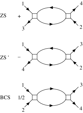
FIG. 1.: The three diagrams contributing to the RG flow at one-loop.

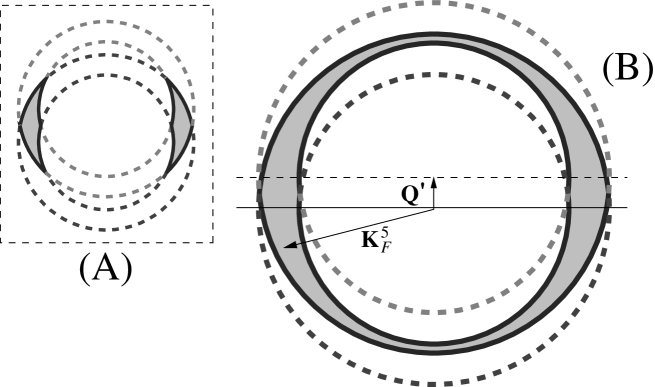
FIG. 2.: If $|{\bf Q}^{\prime}|>2\Lambda$, the intersection (shaded) of the supports of ${\bf K}_{5}$ and ${\bf K}_{5}-{\bf Q}^{\prime}$ are disconnected (A). If $|{\bf Q}^{\prime}|<2\Lambda$, this intersection forms a connected area (B). Note that the RG flow is governed by the boundaries of this intersection, not by their interior directly.

FIG. 3.: (A) Results of the numerical solution of the coupled RG equations. The curves labeled $\Gamma^{*}$ and $F^{*}$ are the forward scattering vertex and the Landau function, respectively, at temperatures $T/v_{F}K_{F}=$ 0.1, 0.025, and 0.01. The narrowest central peak corresponds to the smallest temperature, and vice versa. (B) Approximate analytical solution of the coupled RG equations, for the same parameters as in (A), calculated numerically from Eq. (68). In both cases the initial cutoff was $\Lambda_{0}=K_{F}$.

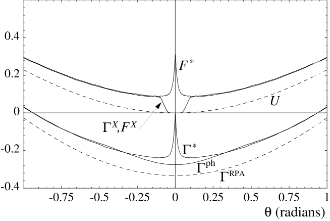
FIG. 4.: Comparison between the exact numerical solution of the coupled RG equations for $T/v_{F}K_{F}=0.005$ ($\Gamma^{*}$ and $F^{*}$), the intermediate values of $\Gamma^{X},F^{X}$ obtained from the initial value $U$ by stopping the flow at $\beta_{R}=5$, and the phenomenological vertex $\Gamma^{\rm ph}$ (the result of the standard FLT derivations) obtained by applying the RPA solution to $\Gamma^{X}$ ($F^{X}$) considered as a new initial point of the flow. $\Gamma^{\rm ph}$ practically coincides with $\Gamma^{*}$, except in the central region.

- [1] L.D. Landau, Sov. Phys. JETP 3, 920 (1957); 5, 101 (1957).
- [2] I.Ia. Pomeranchuk, Zh. Eks. Teor. Fiz. 35, 524 (1958), (English Transl.: Sov. Phys. JETP, 8, 361 (1959)).
- [3] L.D. Landau, Sov. Phys. JETP 8, 70 (1959).
- [4] J.M. Luttinger, Phys. Rev. 119, 1153 (1960).
- [5] A.A. Abrikosov, L.P. Gorkov, and I.E. Dzyaloshinski, 1963, Methods of Quantum Field Theory in Statistical Physics (Dover, New York).
- [6] P. Nozières, 1964, Interacting Fermi Systems (Benjamin, New-York).
- [7] E.M. Lifshitz, L.P. Pitayevskii, 1980, Statistical Physics II (Pergamon Press, Oxford).
- [8] D. Pines, P. Nozières, 1966, The Theory of Quantum Liquids: Normal Fermi Liquids (Addison-Wesley, New York).
- [9] G. Baym and C. Pethick, 1991, Landau Fermi-liquid theory (John Wiley and Sons, New-York).
- [10] A. Houghton and B. Marston, Phys. Rev. B, 48, 7790 (1993); H.-J. Kwon, A. Houghton, and B. Marston, Phys. Rev. B, 52, 8002 (1995); A.H. Castro Neto and E. Fradkin, Phys. Rev. Lett. 72, 1393 (1993); Phys. Rev. B, 51, 4048 (1995). See also references therein.
- [11] F.D.M. Haldane, in Proceedings of the International School of Physics “Enrico Fermi”, 1992, ed. R.A. Broglia and J.R. Schrieffer (North Holland, Amsterdam, 1994).
- [12] G. Benfatto and G. Gallavotti, J. Stat. Phys. 59, 541 (1990); Phys. Rev. B42, 9967 (1990).
- [13] R. Shankar, Physica A 177, 530 (1991).
- [14] J. Polchinski, in Proceedings of the 1992 Theoretical Advanced Studies Institute in Elementary Particle Physics, ed. J. Harvey and J. Polchinski (World Scientific, Singapore, 1993).
- [15] R. Shankar, Rev. Mod. Phys. 66, 129 (1994).
- [16] S. Weinberg, Nucl. Phys. B413 [FS], 567 (1994).
- [17] C. Nayak, F. Wilczek, Nucl. Phys. B417 [FS], 359 (1994); ibid. B430 [FS], 534; cond-mat/9507040.
- [18] A. C. Hewson, Adv. Phys. 43, 543 (1994).
- [19] G.Y. Chitov and D. Sénéchal, Phys. Rev. B 52, 13487 (1995).
- [20] N. Dupuis and G.Y. Chitov, Phys. Rev. B, 54, 3040 (1996).
- [21] A. Stern and B.I. Halperin, Phys. Rev. B 52, 5890 (1995).
- [22] B.I. Halperin, P.A. Lee and N. Read, Phys. Rev. B 47, 7312 (1993)
- [23] The latter point is challenged in some studies predicting a finite effective mass, like, e.g., the bosonization approach of P. Kopietz and G.E. Castilla, Phys. Rev. Lett. 78, 314 (1997). This question deserves further study.
- [24] N.D. Mermin, Phys. Rev. 159, 161 (1967).
- [25] For a comprehensive introduction into the effective action formalism in the present context of fermion systems and other useful issues we recommend a recent review of W. Metzner, C. Castellani and C. Di Castro, cond-mat/9701012.
- [26] N. Dupuis, cond-mat/9604189.
- [27] Both the contribution and the zero-angular part of the contribution become singular in the limit since .
- [28] See, for instance, J. Voit, Rep. Prog. Phys. 58, 977 (1995).
- [29] At exactly zero temperature the angular features of the vertices reduce to finite discontinuities at zero angle, accompanied by finite-angle deviations from the RPA curve depending on the parameters of the effective action, e.g., the radius of Fermi surface, the strength of the interaction, etc. The zero-temperature limit is, however, mostly an academic question since the effect of interference between the Landau and the BCS channels, neglected in this study, would result in a Kohn-Luttinger instability in the -interaction function[15] and destroy the regime of Fermi liquid before the system attains . Due to this second interference our results are not reliable near , since .[15, 19]