Frustrated Systems: Ground State Properties via Combinatorial Optimization

Abstract

An introduction to the application of combinatorial optimization methods to ground state calculations of frustrated, disordered systems is given. We discuss the interface problem in the random bond Ising ferromagnet, the random field Ising model, the diluted antiferromagnet in an external field, the spin glass problem, the solid-on-solid model with a disordered substrate and other convex cost flow problems occurring in superconducting flux line lattices and traffic flow networks. On the algorithmic side we present a concise introduction to a number of elementary algorithms in combinatorial optimization, in particular network flows: the shortest path algorithm, the maximum-flow algorithms and minimum-cost-flow algorithms. We present a short glance at the minimum weighted matching and branch-and-cut algorithms.

Contents

1. What are frustrated systems?

2. What is special for computer simulations of disordered systems?

3. What can you learn from ground state calculations?

4. Ground state interface in a random medium.

5. The random field Ising model.

6. The diluted antiferromagnet in an external field.

7. The spin glass problem.

8. The SOS (solid-on-solid) model on a disordered substrate.

9. Vortex glasses and traffic flows.

10. Appendix: Concepts in network flows and basic algorithms.
    

    • Maximum flow / minimum cut problem.

      • Basic definitions.

      • Residual network and generic augmenting path algorithm.

      • Cuts, labeling algorithm and max-flow-min-cut theorem.

      • Generic Preflow-push algorithm.

    • Shortest path problem.

      • Dijkstra’s algorithm.

      • Label correcting algorithm.

    • Minimum cost flow problem.

      • Definition.

      • Negative cycle canceling algorithm.

      • Reduced cost optimality.

      • Successive shortest path algorithm.

      • Convex cost flows.

1 What are frustrated systems?

Frustrated systems are simply systems in which the individual entities that build up the model (like spins, bosons, fermions, monomers, etc.) feel some sort of “frustration” in the literal sense. This means that on their search for a minimal energy configuration at lower and lower temperatures they are not able to satisfy all interactions with one another or with impurities simultaneously.

As an example we consider a model for a directed polymer in a disordered environment

$$H=\underbrace{\sum_{i}(x_{i}-x_{i+1})^{2}}_{\displaystyle\bf(A)}-\underbrace{\sum_{i}V(x_{i})}_{\displaystyle\bf(B)}\;,$$ (1)

where $x_{i}$ is the displacement of the $i$-th monomer and $V(x)$ is a random potential. The first term (A), the elastic energy, tries to make the polymer straight for $T\to 0$, the second term (B) tries to bring the monomers in favorite positions, for which the polymer has to bend. The monomers cannot satisfy both of these demands simultaneously.

Another, more famous example are magnetic spins (for simplicity Ising spins) with ferromagnetic and antiferromagnetic interactions. Consider the Hamiltonian for 4 spins (e.g. an elementary plaquette of a square lattice)

$$H=-\sigma_{1}\sigma_{2}-\sigma_{2}\sigma_{3}-\sigma_{3}\sigma_{4}+\sigma_{4}\sigma_{1}$$ (2)

and try to find a configuration of the Ising spins $\sigma_{i}=\pm 1$ that minimizes this simple energy function. Naively one starts with some value for the first spin, let’s say $\sigma_{1}=+1$, the first term would then imply $\sigma_{2}=+1$, the second $\sigma_{3}=+1$ and the third $\sigma_{4}=+1$. But what about the last term — here $\sigma_{1}=\sigma_{4}+1$ is not the most favorable configuration. Thus it is impossible to satisfy all local interactions at once, this is why Toulouse[toulouse] introduced the concept of frustration for these plaquette occurring naturally in spin glass models. After some thought one finds that many (i.e. 8) different spin configurations for (2) have a minimal energy, but all of them break one bond. This is the notorious frustration induced ground state degeneracy.

This kind of frustration can occur either via quenched disorder (i.e. a random, time-independent distribution of ferromagnetic and antiferromagnetic spin interactions) or without any disorder, for example in the fully frustrated antiferromagnetic Ising model on a triangular lattice. Of course the same problem occurs with XY-spins, like the XY-antiferromagnet on a triangular or Kagomé lattice. In this letter we treat exclusively disorder induced frustration. The determination of ground states of regularly frustrated systems usually do not need such algorithmic tools as discussed in this lecture (see [unfrust] and references therein for a number of examples).

2 What is special for simulations of disordered systems?

As we learned from our simple 4-spin Hamiltonian above, frustration is often responsible for the existence of many degenerate (or nearly degenerate) states and metastable states. Suppose one intends to perform a conventional Monte Carlo simulation with single spin flip heat bath dynamics of such a system. To explore the whole energy landscape in order to find the most favorable configurations one has overcome large energy barriers between the various minima. As a consequence, the relaxation times typically become astronomically large — not only at a possible phase transition (in which case it would be “critical slowing down”), but also below and above. Thus, as is well known in the community of computational physicists (also among experimentalists, by the way) investigating disordered or amorphous materials, the equilibration is nearly impossible for large systems. Our first commandment in this context therefore is

To be modest in system size is mandatory!

Of course everything would be fine if there would be an efficient cluster algorithm at hand, as discussed in this school. However, there are none — with a few exceptional cases. To invent an efficient cluster algorithm for some model, one first has to have a deep understanding of its physics and a knowledge or an intuition about the low lying energy configurations, the excitations etc. Thus, cum grano salis, if you have understood the system to a rather complete extent, you might be ready to formulate a cluster algorithm — with which you can add some precise numbers (critical exponents etc.) to your basic understanding. Unfortunately, after several decades of research we have still not reached this desirable state for most of the interesting disordered systems.

The next observation is that different samples, i.e. different disorder realizations, can have completely different dynamical and static properties. This goes under the name “large sample to sample fluctuations”, which originates in the lack of self averaging in some physical observables. Not all of them show this notorious behavior: the ground state energy, for instance, is well behaved, simply because the various local minima are nearly degenerate, but e.g. spatial correlation functions or susceptibilities are not self averaging quantities. Consider for instance the diluted ferromagnet with site concentration $c$ and imagine the following two extreme situations: On a square lattice with $N$ spins one could distribute $N/2$ spins in such a way that 1) they form a single, compact cluster, or 2) they occupy a sublattice such that none of them has an occupied nearest neighbor site. Obviously the magnetization or susceptibility has completely different characteristics in the two cases: 1) is a bulk ferromagnet of volume $N/2$ and will have a tendency to order ferromagnetically at some temperature $T_{c}$ (in the limit $N\to\infty$), 2) is a collection of isolated spins that will never order.

Thus one easily recognizes that the probability distribution $P_{L}({\cal O})$ of some observable ${\cal O}$ is usually extremely broad, in particular non-Gaussian. Rare events (i.e. disorder configurations with small probability) can have a strong impact on averaged quantities like susceptibilities or autocorrelations. This leads to our second commandment for all investigations of disordered systems:

Sample a huge (!) number of disorder configurations

The study of the probability distribution $P_{L}({\cal O})$ can be more useful than only average values.

3 What can we learn from ground state calculations?

The ground state is the configuration in which the “equilibrated” system settles at exactly zero temperature (if there is more than one, replace state by states). However, $T=0$ is not accessible in the real world, so why should we bother? There is a number of reasons for it, some of them are listed below:

• As long as one is interested in equilibrium properties (and not in relaxational dynamics, aging, etc.) an exact ground state is more valuable than a non-equilibrium low temperature simulation.

• One might expect that some features of the ground state persist at small temperatures (like the domain structure in the three-dimensional random field Ising model [fractal or not?], etc.).

• If the phase transition into an ordered, may be glassy state, happens at $T=0$, one can extract critical exponents from ground state calculations (as for instance in the two-dimensional Ising spin glass).

• If the RG (renormalization group) flow for a finite $T$ transition is governed by a zero-temperature fixed point, one can again extract the critical exponents via ground state calculations (like in the three-dimensional random field Ising model). These are then, if the RG-picture is correct, identical with those for the finite $T$ transition.

• The zero temperature extrapolation of analytical finite $T$ predictions for the glassy phase can be checked explicitly, like in the SOS (solid-on-solid) model with a disordered substrate.

As a motivation this should be enough, in the next section we jump directly in medias res. But before we start: many people think that combinatorial optimization is essentially the traveling salesman problem, only because it is far the most famous problem (see [tsp] for an excellent introduction). This is similar to saying that frustrated disordered systems are essentially spin glasses (actually the traveling salesman problem and the spin glass problem are intimately connected via their complexity). One aim of this lecture is to remove this prejudice and to demonstrate that there are many more problems out there than only spin glasses (or traveling salesmen): algorithmically much easier to handle but equally fascinating. This is also the reason why on the algorithmic side we focus mainly on network flows: with the help of the material presented in the appendix everybody should be able to sit down in front of the computer and to implement efficiently the algorithms discussed there. If someone wants to know it all, i.e. all background material on graph theory, linear programming and network flows, we refer to standard works such as [wilson_bondy, lawler, papa, chvatal, derigs, ahuja].

4 Ground state interface in a random medium

Although it was historically not the first random Ising model that has been investigated with the help of the maximum flow / minimum cut algorithm (this was the random field Ising model, which we shall discuss later), it might be pedagogically more advantageous to start with the random bond Ising model with a boundary induced interface. The reason for the greater intuitive appeal of the latter problem is that the minimum cut, which the algorithm searches, is identical with the minimum energy interface of the physical system, which we search.

The random bond Ising ferromagnet (RBIFM) is defined by

$$H=-\sum_{(ij)}J_{ij}\sigma_{i}\sigma_{j}$$ (3)

with $\sigma_{i}=\pm 1$ Ising spins and $J_{ij}\geq 0$ ferromagnetic interactions strengths between neighboring spins. These are random quenched variables, which means that they are distributed according to some probability distribution and fixed right from the beginning. $(ij)$ denotes nearest neighbor pairs of a $d+1$-dimensional lattice of size $L^{d}\times H$. We denote the coordinates by $i=(x_{1},\ldots,x_{d},y)$.

Since the interactions are all ferromagnetic, the ground state is simply given by $\sigma_{i}=+1$ for all sites $i$ or $\sigma_{i}=-1$ for all sites $i$. Thus, up to now there is disorder, but no frustration in the problem. This changes by the boundary conditions (b.c.) we define now: we apply periodic b.c. in the $x$-directions and fix the spins at $y=1$ to be $+1$ and those at $y=H$ to be $-1$.

$$\sigma_{(x_{1},\ldots,x_{d},y=1)}=+1\quad{\rm and}\quad\sigma_{(x_{1},\ldots,x_{d},y=H)}=-1$$ (4)

This induces an interface through the sample where bonds have to be broken, as indicated in fig. 1. If all bonds would be of the same strength $J_{ij}=J$ we would have the pure Ising model and the interface would simply be a $d$-dimensional hyperplane perpendicular to the $y$-direction, which costs an energy of $JL^{d}$, $J$ for each broken bond. Because of the randomness of the $J_{ij}$ it is energetically more favorable to break weak bonds: the interface becomes distorted and its shape is rough. This model has also been used to describe fractures in materials where the $J_{ij}$ represents the local force needed to break the material and it is assumed that the fracture occurs along the surface of minimum total rupture force.

Figure 1: Two-dimensional random bond Ising model with a binary distribution of interaction strengths $J_{ij}\in\{J_{i},J_{2}\}$ with $J_{1}\gg J_{2}>0$: Thick lattice bonds are strong ($J_{ij}=J_{1}$), broken lattice bonds are weak $J_{ij}=J_{2}$. The left and right boundary spins are connected to two extra spins $\sigma_{s}=+1$ and $\sigma_{t}=-1$, respectively, with infinitely strong bonds. $\nwarrow$ means $\sigma_{i}=+1$, $\searrow$ means $\sigma_{i}=-1$. The dotted line is the resulting interface: in this example it passes only weak bonds, by which it is of minimal energy. It partitions the lattice into up-and down-spins, the bonds (or more precisely: their corresponding forward arcs — see appendix A.3) that intersect the dotted line constitute the set $(S,\overline{S})$ for the ${s}$-${t}$-cut $[S,\overline{S}]$.

How do we solve the task of finding the minimal energy configuration for the interface? First we map it onto a flow problem in a capacitated network (see appendix A for the nomenclature). We introduce two extra sites, a source node ${s}$, which we connect to all spins of the hyperplane $y=1$ with bonds $J_{{s},(x_{1},\ldots,x_{d},y=1)}=J_{\infty}$, and a sink node ${t}$, which we connect to all spins of the hyperplane $y=H$ with bonds $J_{{s},(x_{1},\ldots,x_{d},y=H)}=J_{\infty}$. We choose $J_{\infty}=2\sum_{(ij)}J_{ij}$, i.e. strong enough that the interface cannot pass through a bond involving one of the two extra sites. Now we enforce the b.c. (4) by simply fixing $\sigma_{s}=+1$ and $\sigma_{t}=-1$. The graph underlying the capacitated network we have to consider is now defined by the set of vertices (or nodes)

$$N=\{1,\ldots,L^{d+1}\}\cup\{{s},{t}\}$$ (5)

and the set of edges (or arcs) connecting them

$$A=\{(i,j)|i,j\in N,\;J_{ij}>0\}\;.$$ (6)

Note that we have forward and backward arcs for each pair of interacting sites in the lattice. The capacities $u_{ij}$ of the arcs $(i,j)$ is given by the bond strength $J_{ij}$. For any spin configuration ${\bf\sigma}=(\sigma_{1},\ldots,\sigma_{N})$ we define now

$$S = \{i\in N|\sigma_{i}=+1\}$$ (7)

$$\overline{S} = \{i\in N|\sigma_{i}=-1\}=N\backslash S$$

Obviously $\sigma_{s}\in S$ and $\sigma_{t}\in\overline{S}$. The knowledge of $S$ is sufficient to determine the energy of any spin configuration via (3):

$$H(S) = -\sum_{(i,j)\in E(S)}J_{ij}-\sum_{(i,j)\in E(\overline{S})}J_{ij}+\sum_{(i,j)\in(S,\overline{S})}J_{ij}$$

$$= -C+2\sum_{(i,j)\in(S,\overline{S})}J_{ij}$$

where $E(S)=\{(i,j)|i\in S,j\in S\}$, $E(\overline{S})=\{(i,j)|i\in\overline{S},j\in\overline{S}\}$ and $(S,\overline{S})=\{(i,j)|i\in S,j\in\overline{S}\}$. The constant $C=\sum_{(i,j)\in E(N)}J_{ij}$ is irrelevant (i.e. independent of $S$). Note that $(S,\overline{S})$ is the set of edges (or arcs) connecting $S$ with $\overline{S}$, this means it cuts $N$ in two disjoint sets. Since ${s}\in S$ and ${t}\in\overline{S}$, this is a so called ${s}$-${t}$-cut-set, abbreviated $[S,\overline{S}]$. Thus the problem of finding the ground state of (3) with the interface inducing b.c. (4) can be reformulated as a minimum cut problem

$${\rm min}_{S\subset N}\,\{H^{\prime}(S)\}={\rm min}_{[S,\overline{S}]}\sum_{(i,j)\in(S,\overline{S})}J_{ij}\;.$$ (9)

in the above defined capacitated network (with $H^{\prime}=(H+C)/2$). It does not come as a surprise that this minimum cut is identical with the interface between the ($\sigma_{i}$=+1)-domain and the ($\sigma_{i}$=-1)-domain that has the lowest energy. Actually any ${s}$-${t}$-cut-set defines such an interface, some of them might consist of many components, which is of course energetically unfavorable.

To conclude, we have to find the minimum cut in a capacitated network, which is, as we show in appendix A, equivalent to finding a maximum flow from node ${s}$ to node ${t}$. An intuitive argument for this famous max-flow-min-cut theorem is the following: Suppose you have to push, let’s say waterflow through a network of pipelines, each with some capacity. The capacities in our case are the ferromagnetic interaction strengths on the bonds (pipes) between the nodes. Somewhere in the network there is a bottle-neck (in general consisting of several pipes) which does not allow a further increase of the waterflow sent from the source to the sink. If the maximum possible flow goes through the network, the flow on the pipes of the bottle-neck is equal to their capacity. The minimum cut is simply the global bottle-neck with the smallest capacity, and thus determines the maximum flow.

One can solve the above task by applying the straightforward augmenting path algorithm discussed in appendix A.2, which is based on the idea to find directed paths in the network on which one could possibly send more flow from the source to the sink. If one finds such paths, one augments the flow along them (i.e. pushes more water through the pipes), if there are none, the present flow is optimal. In the latter case one identifies the corresponding ${s}$-${t}$ cut, which then yields the exact ground state interface for the above problem.

A more efficient way is to use the preflow push algorithm presented in appendix A.4. The idea of this algorithm is to flood the network starting from the source. Then one encounters the situation that some nodes are not able to transport the flood coming from the source into the direction of the sink, which means that one has to send some flow back to the source. The time consuming part of this algorithm is the retreat of floods that have been pushed too far, and this retreat happens faster if the capacities of backwards arcs is as large as possible. Bearing this observation in mind Middleton [middleton] has suggested a nice modification of the original problem that yields a significant speed up: to forbid overhangs of the interface we are discussing is equivalent to introduce backward arcs with infinite capacity in the corresponding flow network (obviously a minimum cut will then never contain such an arc as forward arc). Thus, in the case that too much flow has been pushed, the retreat works with maximum efficiency.

To conclude let us cite a number of results that have been obtained in this way. Of particular interest here is the width of the interface

$$W(L,H)=([y_{x}^{2}]_{\rm av}-[y_{x}]_{\rm av}^{2})^{1/2}\sim L^{\zeta}\tilde{w}(H/L^{\zeta})\;,$$ (10)

where $y_{x}$ is the $y$-coordinate of the point $(\underline{x},y)$ of the interface (note that because of the “no overhangs” prescription $y_{x}$ is single-valued). $[\ldots]_{\rm av}$ means an average over the disorder. One expects the finite size scaling form as indicated with a roughness exponent $\zeta$. From the ground state calculations and finite size scaling one finds [middleton] that $\zeta=0.41\pm 0.01$ in 2d ($L$ up to 120, and $H$ up to 50, with $10^{3}-10^{4}$ samples), and $\zeta=0.22\pm 0.01$ in 3d ($L$ up to 30 and $H$ up to 20).

5 The random field Ising model

The random field Ising model (RFIM, for a review see [rieger_review]) is defined

$$H=-\sum_{(ij)}J_{ij}\sigma_{i}\sigma_{j}-\sum_{i}h_{i}\sigma_{i}$$ (11)

with $\sigma_{i}=\pm 1$ Ising spins, ferromagnetic bonds $J_{ij}\geq 0$ (random or uniform), $(ij)$ nearest neighbor pairs on a $d$-dimensional lattice and at each site $i$ a random field $h_{i}\in R$ that can be positive and negative. The first term prefers a ferromagnetic order, which means it tries to align all spins. The random field, however, tends to align the spins with the field which points in random directions depending on whether it is positive or negative. This is the source of frustration in this model.

Let us suppose for the moment uniform interactions $J_{ij}=J$ and a symmetric distribution of the random fields with mean zero and variance $h_{r}$. It is established by now that in 3d (and higher dimensions) the RFIM shows ferromagnetic long range order at low temperatures, provided $h_{r}$ is small enough. In 1d and 2d there is no ordered phase at any finite temperature. Thus in 3d one has a paramagnetic/ferromagnetic phase transition along a line $h_{c}(T)$ in the $h_{r}$-$T$-diagram.

The renormalization group (RG) picture says that the nature of the transition is the same all along the line $h_{c}(T)$, with the exception being the pure fixed point at $h_{r}=0$ and $T_{c}\sim 4.51J$. The RG flow is dominated by a zero temperature fixed point at $h_{c}(T$=$0)$. As a consequence, the critical exponents determining the critical behavior of the RFIM should be all identical along the phase transition line, in particular identical to those one obtains at zero temperature by varying $h_{r}$ alone.

Therefore we consider zero temperature from now on. Close to the transition at $h_{c}=h_{c}(T$=$0)$ one would e.g. expect for the disconnected susceptibility

$$\chi_{\rm dis}=\frac{1}{L^{3}}\biggl{[}\sum_{i,j}\sigma_{i}\sigma_{j}\biggr{]}_{\rm av}\sim L^{4-\overline{\eta}}\tilde{\chi}(L^{1/\nu}\delta)$$ (12)

where $\delta=h_{r}-h_{c}$ is the distance from the critical point and $\nu$ is the thermal critical exponent. An analogous expression holds for the magnetization involving the exponent $\beta$. Thus to estimate a set of critical exponents the task is to calculate the ground state configurations of the RFIM (11).

This optimization task is again equivalent to a maximum flow problem [barahona_rfim], as in the interface model discussed in the last section. Historically the RFIM was the first physical model that has been investigated with a maximum flow algorithm [ogielski]. However, here the minimum-cut is not a geometric object within the original system and therefore we found it more intuitive to discuss the RFIM after the interface problem.

In essence we proceed in the same way as in the last section. Again we add to extra nodes ${s}$ and ${t}$ and put spins with fixed values there:

$$\sigma_{s}=+1\quad{\rm and}\qquad\sigma_{t}=-1$$ (13)

We connect all sites with positive random field to the node ${s}$ and all sites with negative random field to ${t}$:

$$\begin{array}[]{lcl}J_{{s}i}&=&\left\{\begin{array}[]{lcl}h_{i}&&{\rm if}\;h_{i}\geq 0\\ 0&&{\rm if}\;h_{i}<0\end{array}\right.\\ J_{i{t}}&=&\left\{\begin{array}[]{lcl}|h_{i}|&&{\rm if}\;h_{i}<0\\ 0&&{\rm if}\;h_{i}\geq 0\end{array}\right.\end{array}$$ (14)

We construct a network with the set of nodes $N=\{1,\cdots,L^{d}\}\cup\{{s},{t}\}$ and the set of (forward and backward) arcs $A=\{(i,j)|\,i,j\in N,\;J_{ij}>0\}$. Each of them has a capacity $u_{ij}=J_{ij}$. Now we can write the energy or cost function as

$$E=-\sum_{(i,j)\in A}J_{ij}\sigma_{i}\sigma_{j}$$ (15)

and, by denoting the set $S=\{i\in N|S_{i}=+1\}$ and $\overline{S}=N\backslash S$ the energy can be written as in equation (4):

$$E(S)=-C+2\sum_{(i,j)\in(S,\overline{S})}J_{ij}$$ (16)

with $C=\sum_{(i,j)\in A}J_{ij}$. The problem is reduced to the problem of finding a minimum ${s}$-${t}$-cut as in (9). The difference to the interface problem is that now the extra bonds connecting the two special nodes ${s}$ and ${t}$ with the original lattice do not have infinite capacity: they can lie in the cut, namely whenever it is more favorable not to break a ferromagnetic bond but to disalign a spin with its local random field. In the extended graph which we consider the ${s}$-${t}$-cut again forms connected interface, however, in the original lattice (without the bonds leading to and from the extra nodes) the resulting structure is generally disconnected, a multicomponent interface. Each single component surrounds a connected region in the original lattice containing spins, which all point in the same direction. In other words, they form ferromagnetically ordered domains separated by domain walls given by the subset of the ${s}$-${t}$-cut that lies in the original lattice.

The maximum flow algorithm has been used by Ogielski [ogielski] to calculate the critical exponents of the RFIM via the above mentioned finite size scaling. He obtained

$$\nu=1.0\pm 0.1\;,\qquad\overline{\eta}=1.1\pm 0.2\;,\qquad\beta\approx 0.05$$ (17)

with $\beta$ being so small that it is (numerically) indistinguishable from zero, indicating a discontinuous transition. These estimates are compatible with those obtained by recent Monte Carlo simulations supporting the RG idea of the universality of the transition at finite and zero temperature. However, this is still not the end of the story, since various scaling predictions, also based on the RG picture, are violated. For further details we refer to the review [rieger_review].

6 The diluted antiferromagnet in an external field

Experimentally it is of course hard to prepare a random field at each lattice site, therefore one might ask why people have been so enthusiastic about the RFIM, discussed in the last section, over decades. Actually it is because within a field theoretic perturbation theory (around small random fields) it has been shown [fishman] that the RFIM is in the same universality class as the diluted antiferromagnet in a uniform magnetic field (DAFF) defined via

$$H=+\sum_{(ij)}J_{ij}\varepsilon_{i}\varepsilon_{j}\sigma_{i}\sigma_{j}-\sum_{i}h_{i}\varepsilon_{i}\sigma_{i}$$ (18)

where $\sigma_{i}=\pm 1$, $J_{ij}\geq 0$, $(ij)$ are nearest neighbor pairs on a simple cubic lattice, and $\varepsilon_{i}\in\{0,1\}$ with $\varepsilon_{i}=1$ with probability $c$, representing the concentration of spins. Usually one takes $J_{ij}=J$ and $h_{i}=h$, both uniform. Because of the plus sign in front of the first term in (18) all interactions are antiferromagnetic, the model represents a diluted antiferromagnet, for which many experimental realizations exist (e.g. Fe_cZn_1-cF₂). Now that neighboring spins tend to point in opposite directions due to their antiferromagnetic interaction a uniform field competes with this ordering tendency by trying to align them all. Thus it is again a frustrated system. Due to the analogy to the RFIM model one expects at low temperatures and small enough fields a second order phase transition from a paramagnetic to an antiferromagnetic phase.

In recent years people began to doubt the folklore that the DAFF is under all circumstances a good experimental realization of the RFIM model. Note that this result has been derived for small fields $h$, and the question is whether this still holds at larger fields. The largest field value at which the paramagnetic-antiferromagnetic transition can be studied is $h_{c}(T=0)$. This motivates the study of the ground state transition along the same lines as in the RFIM context. Preliminary results [esser] indicate that the critical exponents are different here, which implies that the RFIM and the DAFF are in different universality classes at large field values.

Here we are primarily interested in the question whether we can again map the calculation of ground states onto a maximum flow problem, as for the RFIM. The answer is yes as long as the antiferromagnetic interactions are short ranged among nearest neighbors on a bipartite lattice. With zero external field the ground state would be antiferromagnetic, which means (remember we have a simple cubic lattice) that we can define two bipartite sublattices $A$ and $B$ like the black and white fields of a checkerboard. Each site $i$ in $A$ finds all its nearest neighbors $j$ in $B$ and vice versa. Define new spin and field variables via

$$\sigma_{i}^{\prime}=\left\{\begin{array}[]{lcl}+\sigma_{i}&\quad{\rm for}&i\in A\\ -\sigma_{i}&\quad{\rm for}&i\in B\end{array}\right.\quad,\quad h_{i}^{\prime}=\left\{\begin{array}[]{lcl}+\varepsilon_{i}h_{i}&\quad{\rm for}&i\in A\\ -\varepsilon_{i}h_{i}&\quad{\rm for}&i\in B\end{array}\right.\;.$$

Since $\sigma_{i}^{\prime}\sigma_{j}^{\prime}=-\sigma_{i}\sigma_{j}$ for all nearest neighbor pairs $(ij)$ one can write (18) as

$$H=-\sum_{(ij)}J_{ij}^{\prime}\sigma_{i}^{\prime}\sigma_{j}^{\prime}-\sum_{i}h_{i}^{\prime}\sigma_{i}^{\prime}$$ (19)

with $J_{ij}^{\prime}=J_{ij}\varepsilon_{i}\varepsilon_{j}$. Now the Hamiltonian has exactly the same form as the one for the RFIM, since $J^{\prime}_{ij}\geq 0$. Note that even if one starts with uniform bonds $J_{ij}=J$ and a uniform field $h_{i}=h$ the dilution generates bond- and field disorder! Now that one has reduced the problem to the RFIM we also know how to map it to a maximum flow problem. Hartmann and Usadel [hartmann] have extended the algorithm in such a way that all ground states can be calculated: for uniform bonds and fields the resulting RFIM has a discrete distribution of random bonds and fields, which leads in general to a high degeneracy of the ground state, something that does not happen in case of a uniform distribution, where usually the ground state is unique.

In this context we would like to mention the Coulomb glass model [shklovsky, tenelsen], which is a model for point charges on a $d$-dimensional lattice with long-range Coulomb interactions (repulsive of strength $V/r$ with $V$ positive and $r$ being the Euclidean distance between two charges):

$$H=\sum_{i,j}\frac{V}{r_{ij}}n_{i}n_{j}+\sum_{i}n_{i}\mu_{i}$$ (20)

where now the sum is over all pairs of sites of the lattice. $n_{i}\in\{0,1\}$ indicates the presence ($n_{i}=1$) or absence ($n_{i}=0$) of a charged particle at site $i$ and $r_{ij}$ is the Euclidean distance between site $i$ and site $j$. The random local potentials $\mu_{i}\in[-W,W]$ represent the quenched disorder. Obviously this model is equivalent to an antiferromagnet with long-range interactions and random fields. Up to now no way of mapping this interesting problem onto a network flow problem is known, it seems to fall into the spin glass class, which we discuss now.

7 The spin glass problem

Spin glasses are the prototypes of (disordered) frustrated systems, their history is quite a long one and for the present status of numerical investigation I refer to [rieger_review], where also numerous references to experimental and theoretical introductions can be found. In the models we discussed up to now, the frustration was caused by two separate terms of different physical origin (interactions and external fields or boundary conditions). Spin glasses are magnetic systems in which the magnetic moments interact ferro- or antiferromagnetically in a random way, as in the following Edwards-Anderson Hamiltonian for a short ranged Ising spin glass (SG)

$$H=-\sum_{(ij)}J_{ij}\sigma_{i}\sigma_{j}\;,$$ (21)

where $\sigma_{i}=\pm 1$, $(ij)$ are nearest neighbor interactions on a $d$-dimensional lattice and the interaction strengths $J_{ij}\in R$ are unrestricted in sign. In analogy to eq. (4–9) one shows that the problem of finding the ground state is again equivalent to finding a minimal cut $[S,\overline{S}]$ in a network

$${\rm min}_{\bf\underline{\sigma}}\,\{H^{\prime}({\bf\underline{\sigma}})\}={\rm min}_{[S,\overline{S}]}\sum_{(i,j)\in(S,\overline{S})}J_{ij}\;,$$ (22)

again $H^{\prime}=(H+C)/2$ with $C=\sum_{(ij)}J_{ij}$. However, now the capacities $u_{ij}=J_{ij}$ of the underlying network are not non-negative any more, therefore it is not a minimum-cut problem in the sense of appendix A.3 and thus it is also not equivalent to a maximum flow problem, which we know how to handle efficiently.

It turns out that the spin glass problem is much harder than the questions we have discussed so far. In general (i.e. in any dimension larger than two and also for 2d in the presence of an external field) the problem of finding the SG ground state is ${\cal NP}$-complete [barahona], which means in essence that no polynomial algorithm for it is known (and also that chances to find one in the future are marginal). Nevertheless, some extremely efficient algorithms for it have been developed [groetschel, juenger, kobe], which have a non-polynomial bound for their worst case running-time but which terminate (i.e find the optimal solution) after a reasonable computing time for pretty respectable system sizes.

First we discuss the only non-trivial case that can be solved with a polynomial algorithm: the two-dimensional Ising SG on a planar graph. This problem can be shown to be equivalent to finding a minimum weight perfect matching, which can be solved in polynomial time. We do not treat matching problems and the algorithms to solve them in this lecture (see [lawler, papa, derigs]), however, we would like to present the idea [barahona]. To be concrete let us consider a square lattice with free boundary conditions. Given a spin configuration ${\bf\underline{\sigma}}$ (which is equivalent to $-{\bf\underline{\sigma}}$) we say that an edge (or arc) $(i,j)$ is satisfied if $J_{ij}\sigma_{i}\sigma_{j}>0$ and it is unsatisfied if $J_{ij}\sigma_{i}\sigma_{j}<0$. Furthermore we say a plaquette (i.e. a unit cell of the square lattice) is frustrated if it is surrounded by an odd number of negative bonds (i.e. $J_{ij}\cdot J_{jk}\cdot J_{kl}\cdot J_{li}<0$ with $i$, $j$, $k$ and $l$ the four corners of the plaquette)). There is a one-to-one correspondence between equivalent spin configurations (${\bf\underline{\sigma}}$ and $-{\bf\underline{\sigma}}$) and sets of unsatisfied edges with the property that on each frustrated (unfrustrated) plaquette there is an odd (even) number of unsatisfied edges. See fig. 2 for illustration.

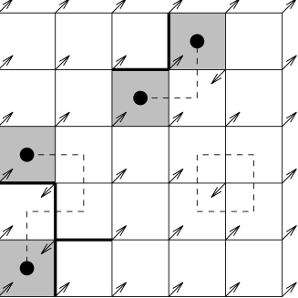
Figure 2: Two-dimensional Ising spin glass with $\pm$-J couplings: Thin lines, are positive interactions, thick lines are negative interactions, $\nearrow$ means $\sigma_{i}=+1$, $\swarrow$ means $\sigma_{i}=-1$, shaded faces are frustrated plaquettes, broken lines cross unsatisfied edges.

Note that

$$H({\bf\underline{\sigma}})=-C+2\sum_{\rm unsatisfied\;edges}|J_{ij}|\;.$$ (23)

which means that one has to minimize the sum over the weights of unsatisfied edges. A set of unsatisfied edges will be constituted by a set of paths (in the dual lattice) from one frustrated plaquette to another and a set of closed circles (see fig. 2). Obviously the latter always increase the energy so that we can neglect them. The problem of finding the ground state is therefore equivalent to finding the minimum possible sum of the weights of these paths between the frustrated plaquettes. This means that we have to match the black dots in the fig. 2 with one another in an optimal way. One can map this problem on a minimum weight perfect matching problem, which can be solved in polynomial time (see [barahona] for further details).

Note that for binary couplings, i.e. $J_{ij}=\pm J$, where $J_{ij}=+J$ with probability $p$ the weight of a matching is simply proportional to the sum of the lengths of the various paths connecting the centers of the frustrated plaquettes, which simplifies the actual implementation of the algorithm. In [kawashima] the 2d $\pm J$ spin glass and the site disordered SG has been studied extensively with this algorithm.

As we mentioned, in any other case except the planar lattice situation discussed above the spin glass problem is $\cal NP$-hard. In what follows we would like to sketch the idea of an efficient but non-polynomial algorithm [juenger, diehl]. To avoid confusion with the minimum cut problem we discussed in connection with maximum flows one calls the problem (22) a max-cut problem (since finding the minimum of $H$ is equivalent to finding the maximum of $-H$).

Let us consider the vector space $R^{A}$. For each cut $[S,\overline{S}]$ define $\chi^{(S,\overline{S})}\in R^{A}$, the incidence vector of the cut, by $\chi_{e}^{(S,\overline{S})}=1$ for each edge $e=(i,j)\in(S,\overline{S})$ and $\chi_{e}^{(S,\overline{S})}=0$ otherwise. Thus there is a one-to-one correspondence between cuts in $G$ and their $\{0,1\}$-incidence vectors in $R^{A}$. The cut-polytope $P_{C}(G)$ of $G$ is the convex hull of all incidence vectors of cuts in $G$: $P_{C}(G)={\rm conv}\;\{\chi^{(S,\overline{S})}\in R^{A}\,|\,S\subseteq A\}$. Then the max-cut problem can be written as a linear program

$${\rm max}\,\{\underline{u}^{T}\underline{x}\,|\,\underline{x}\in P_{C}(G)\}$$ (24)

since the vertices of $P_{C}(G)$ are cuts of $G$ and vice versa. Linear programms usually consist of a linear cost function $\underline{u}^{T}\underline{x}$ that has to be maximized under the constraint of various inequalities defining a Polytope in $R^{n}$ (i.e. the convex hull of finite subsets of $R^{n}$) and can be solved for example by the simplex method, which proceeds from corner to corner of that polytop to find the maximum (see e.g. [lawler, chvatal, derigs]). The crucial problem in the present case is that it is $\cal NP$-hard to write down all inequalities that represent the cut polytop $P_{C}(G)$.

It turns out that also partial systems are useful, and this is the essential idea for an efficient algorithm to solve the general spin glass problem as well as the traveling salesman problem or other so called mixed integer problems (i.e. linear programms where some of the variables $x$ are only allowed to take on some integer values, like 0 and 1 in our case) [tsp, thienel]. One chooses a system of linear inequalities $L$ whose solution set $P(L)$ contains $P_{C}(G)$ and for which $P_{C}(G)={\rm convex\;hull}\,\{{\bf x}\in P(L)|x\,\,{\rm integer}\}$. In the present case these are $0\leq x\leq 1$, which is trivial, and the so called cycle inequalities, which are based on the observation that all cycles in $G$ have to intersect a cut an even number of times (have a look at the cut in fig. 1 and choose as cycles for instance the paths around elementary plaquettes). The most remarkable feature of this set $L$ of inequalities is that the separation problem for them can be solved in polynomial time: the cutting plane algorithm which, starting from some small initial set of inequalities, generates iteratively new inequalities until the optimal solution for the actual subset of inequalities is feasible. Note that one does not solve this linear programm by the simplex method since the cycle inequalities are still too numerous for this to work efficiently.

Due to the insufficient knowledge of the inequalities that are necessary to describe $P_{C}(G)$ completely, one may end up with a nonintegral solution ${\bf x}^{*}$. In this case one branches on some fractional variable $x_{e}$ (i.e. a variable with $x_{e}^{*}/\!\!\!\!\!\in\{0,1\}$), creating two subproblems in one of which $x_{e}$ is set to 0 and in the other $x_{e}$ is set to 1. Then one applies the cutting plane algorithm recursivley for both subproblems, which is the origin of the name branch-and-cut. Note that in principle this algorithm is not restricted to any dimension, boundary conditions, or to the fieldless case. However, there are realizations of it that run fast (e.g. in 2d) and others that run slow (e.g. in 3d) and it is ongoing research to improve on the latter. A detailed description of the rather complex algorithm can be found in [thienel, diehl].

The typical questions one tries to address in the context of spin glasses is: is there a spin glass transition at finite temperature, below which the spins freeze into some configuration (i.e. $\langle\sigma_{i}\rangle_{T}\neq 0$ for $T<T_{c}$). What can we do with ground state calculation to answer this question? Here the concept of the domain wall energy plays a crucial role [bray]. What a finite but small temperature does is to destroy the ground state order by collectively flipping larger and larger clusters (droplets). If the energy cost for a reversal of a cluster of linear size $L$ increases with $L$ (like $\Delta E\propto L^{y}$ with $y>0$) thermal fluctuation will not be able to destroy long range order, and thus we have a spin glass transition at finite $T_{c}$. If it decreases (i.e. $y<0$) long range order is unstable with respect to thermal fluctuations and the spin glass state occurs only at $T=0$. As an example consider the $d$-dimensional pure Ising ferromagnet, for which the ground state is all spins up or all down. Reversing a cluster of linear size $L$ breaks all surface bonds of this cluster, which means that it costs an energy $\Delta E\propto L^{d-1}$, i.e. $y=d-1$ for the pure ferromagnet. Thus the ferromagnetic state in pure Ising systems is stable for $d>1$, which is well known. Instead of reversing spins one usually studies the energy difference between ground states for periodic and antiperiodic boundary conditions. In [rieger_sg] it has been shown that

$$\Delta E\sim L^{y}$$ (25)

with $y=-0.281$ for the 2d Ising spin glass with a uniform distribution (thus there is no finite $T$ SG transition in this case). It has been speculated that in the $\pm J$ case for a range of concentration of ferromagnetic bonds [antiphase] and in the site-random case for some concentration of $A$ atoms [siterandom] a spin glass phase might exist at non-zero temperature $T>0$. This possibility has been ruled out in [kawashima] with the help of ground state calculations.

With the above mentioned branch & cut algorithm the magnetic field dependence of the ground state magnetization $m_{L}(h)=L^{-d}[|\sum_{i}\sigma_{i}|]_{\rm av}$ has been calculated in the 2d case with a uniform coupling distribution. In [rieger_sg] it has been shown that it obeys finite size scaling form

$$m_{L}(h)\sim L^{-d/2}\tilde{m}(Lh^{1/\delta})$$ (26)

(note $d=2$) with $\delta=1.481$. This value is remarkable in so far as it clearly violates the scaling prediction $\delta=1-y$.

Finally we would like to focus our attention on the very important concept of chaos in spin glasses. This notion implies an extreme sensitivity of the SG-state with respect to small parameter changes like temperature or field variations. There is a length scale $\lambda$ — the so called overlap length — beyond which the spin configurations within the same sample become completely decorrelated if compared for instance at two different temperatures

$$C_{\Delta T}:=[\langle\sigma_{i}\sigma_{i+r}\rangle_{T}\langle\sigma_{i}\sigma_{i+r}\rangle_{T+\Delta T}]_{\rm av}\sim\exp\Bigl{(}-r/\lambda(\Delta T)\Bigr{)}\;.$$ (27)

This should also hold for the ground states if one slightly varies the interaction strengths $J_{ij}$ in a random manner with amplitude $\delta$. Let ${\bf\underline{\sigma}}$ be the ground state of a sample with couplings $J_{ij}$ the ground state of a sample with couplings $J_{ij}+\delta K_{ij}$, where the $K_{ij}$ are random (with zero mean and variance one) and $\delta$ is a small amplitude. Now define the overlap correlation function as

$$C_{\delta}(r):=[\sigma_{i}\sigma_{i+r}\,\sigma_{i}^{\prime}\sigma_{i+r}^{\prime}]_{\rm av}\;\sim\;\tilde{c}(r\delta^{1/\zeta})\;,$$ (28)

where the last relation indicates the scaling behavior we would expect (the overlap length being $\lambda\sim\delta^{-1/\zeta}$) and $\zeta$ is the chaos exponent. In [rieger_sg] this scaling prediction was confirmed with $1/\zeta=1.2\pm 0.1$.

8 The SOS-model on a disordered substrate

Up to now we have considered Ising models exclusively. Quite recently it has been shown [blasum, rieger_sos] that many more frustrated systems are amenable to ground state studies of the kind we discussed so far. Consider a solid-on-solid model with random offsets, modeling a crystalline surface on a disordered substrate as indicated in fig. 3. It is defined by the following Hamiltonian (or energy function):

$$H=\sum_{(ij)}f(h_{i}-h_{j})$$ (29)

where $(ij)$ are nearest neighbor pairs on a $d$–dimensional lattice ($d=1,2$) and $f(x)$ is an arbitrary convex ($f^{\prime\prime}(x)\geq 0$) and symmetric ($f(x)=f(-x)$) function, for instance $f(x)=x^{2}$. Each height variable $h_{i}=d_{i}+n_{i}$ is the sum of an integer particle number which can also be negative, and a substrate offset $d_{i}\in[0,1[$. For a flat substrate, $d_{i}=0$ for all sites $i$, we have the well known SOS-model [puresos]. The disordered substrate is modeled by random offsets $d_{i}\in[0,1[$ [tsai], which are distributed independently.

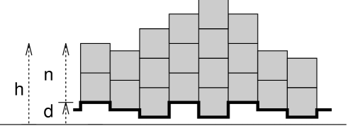
Figure 3: The SOS model on a disordered substrate. The substrate heights are denoted by $d_{i}\in[0,1]$, the number of particle on site $i$ by $n_{i}\in Z$, which means that they could also be negative, and the total height on site $i$ by $h_{i}=d_{i}+n_{i}$

The model (29) has a phase transition at a temperature $T_{c}$ from a (thermally) rough phase for $T>T_{c}$ to a super-rough low temperature phase for $T<T_{c}$. In two dimension ”rough” means that the height-height correlation function diverges logarithmically with the distance $C(r)=[\langle(h_{i}-h_{i+r})^{2}\rangle]_{\rm av}=a\cdot T\cdot\log(r)$ (with $a=1/\pi$ for $f(x)=x^{2}$), ”super-rough” means that either the prefactor on front of the logarithm is significantly larger than $a\cdot T$, or that $C(r)$ diverges faster than $\log(r)$, e.g. $C(r)\propto\log^{2}(r)$.

A part of the motivation to study this model thus comes from its relation to flux lines in disordered superconductors, in particular high-T_c superconductors: The phase transition occurring for (29) is in the same universality class as a flux line array with point disorder defined via the two-dimensional Sine-Gordon model with random phase shifts

$$H=-\sum_{(ij)}(\phi_{i}-\phi_{j})^{2}-\lambda\sum_{i}\cos(\phi_{i}-\theta_{i})\>,$$ (30)

where $\phi_{i}\in[0,2\pi[$ are phase variables, $\theta_{i}\in[0,2\pi[$ are quenched random phase shifts and $\lambda$ is a coupling constant. One might anticipate that both models (29) and (30) are closely related by realizing that both have the same symmetries (the energy is invariant under the replacement $n_{i}\to n_{i}+m$ ($\phi_{i}\to\phi_{i}+2\pi m$) with $m$ an integer). Close to the transition one can show that all higher order harmonics apart from the one present in the Sine-Gordon model (30) are irrelevant in a field theory for (29), which establishes the identity of the universality classes.

To calculate the ground states of the SOS model on a disordered substrate with general interaction function $f(x)$ we map it onto a minimum cost flow model. Let us remark, however, that the special case $f(x)=|x|$ can be mapped onto the interface problem in the random bond Ising ferromagnet in 3d with columnar disorder [zeng] (i.e. all bonds in a particular direction are identical), by which it can be treated with the maximum flow algorithm we know already.

We define a network $G$ by the set of nodes $N$ being the sites of the dual lattice of our original problem and the set of directed arcs $A$ connecting nearest neighbor sites (in the dual lattice) $(i,j)$ and $(j,i)$. If we have a set of height variables $n_{i}$ we define a flow ${\bf x}$ in the following way: Suppose two neighboring sites $i$ and $j$ have a positive (!) height difference $n_{i}-n_{j}>0$. Then we assign the flow value $x_{ij}=n_{i}-n_{j}$ to the directed arc $(i,j)$ in the dual lattice, for which the site $i$ with the larger height value is on the right hand side, and assign zero to the opposite arc $(j,i)$, i.e. $x_{ji}=0$. And also $x_{ij}=0$ whenever site $i$ and $j$ are of the same height. See fig. 4 for a visualization of this scheme. Obviously then we have:

$$\forall i\in N\;:\qquad\sum_{\{j\,|\,(i,j)\in A\}}x_{ij}=\sum_{\{j\,|\,(j,i)\in A\}}x_{ji}\;.$$ (31)

On the other hand, for an arbitrary set of values for $x_{ij}$ the constraint (31) has to be fulfilled in order to be a flow, i.e. in order to allow a reconstruction of height variables out from the height differences. This observation becomes immediately clear by looking at fig. 4.

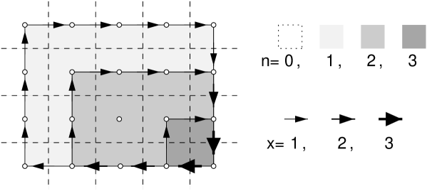
Figure 4: The flow representation of a surface (here a ”mountain” of height $n_{i}=3$). The broken lines represent the original lattice, the open dots are the nodes of the dual lattice. The arrows indicate a flow on the dual lattice, that results from the height differences of the variables $n_{i}$ on the original lattice. Thin arrows indicate a height difference of $x_{ij}=1$, medium arrows $x_{ij}=2$ and thick arrows $x_{ij}=3$. According to our convention the larger height values are always on the right of an arrow. Observe that on each node one the mass balance constraint (31) is fulfilled.

We can rewrite the energy function as

$$H({\bf x})=\sum_{(i,j)}h_{ij}(x_{ij})\;,\qquad{\rm with}\qquad c_{ij}(x)=f(x-d_{ij})\;,$$ (32)

with $d_{ij}=d_{i}-d_{j}$. Thus our task is to minimize $H({\bf x})$ under the constraint (31), which is (see appendix C.5) a minimum-cost-flow problem with the mass balance constraints (31) and arc convex cost functions $h_{ij}(x_{ij})$. It is worth mentioning that this mapping from the SOS model to a flow problem is closely related to the dual link representation of the XY-model in two dimensions [kleinert]. This does not come as a great surprise since we already pointed out the relationship with the Sine-Gordon Hamiltonian involving phase variables (30).

The most straightforward way to solve this problem is to start with all height variables set to zero (i.e. ${\bf x}=0$) and then to look for regions (or clusters) that can be increased collectively by one unit with a gain in energy. This is essentially what the negative cycle canceling algorithm discussed in appendix C.5 does: The negative cycles in the dual lattice surround the regions in which the height variables should be increased or decreased by one. However, it turns out that this is a non-polynomial algorithm, the so called successive shortest path algorithm is more efficient and solves this problem in polynomial time, see appendix C.5. This algorithm starts with an optimal solution for $H({\bf x})$, which is given by $x_{ij}=+1$ for $d_{ij}>1/2$, $x_{ij}=-1$ for $d_{ij}<-1/2$ and $x_{ij}=0$ for $d_{ij}\in[-1/2,+1/2]$. Since this set of flow variables violates the mass balance constraints (31) (in general there is some imbalance at the nodes) the algorithm iteratively removes the excess/deficit at the nodes by augmenting flow.

Let us briefly summarize the results one obtains by applying this algorithm to the ground state problem for the SOS model on a disordered substrate [rieger_sos]:

• The height-height correlation function diverges like $C(r)\propto\log^{2}(r)$ with the distance $r$.

• $\chi_{L}=L^{-4}\sum_{i,j}[(h_{i}-h_{j})^{2}]_{\rm av}$ can nicely be fitted to $\chi_{L}=a+b\log(L)+c\log^{2}(L)$, indicating again a $\log^{2}$ dependence of the height-height correlation function. Moreover, the coefficients $a$, $b$ and $c$ depend on the power $n$ in $f(x)=|x|^{n}$: $c$ increases systematically with increasing $n$.

• By considering a boundary induced step in the ground state configuration one sees that the step energy increases algebraically with the system size: $\Delta E\sim L^{y}$ with $y=0.45\pm 0.05$. This corresponds to the domain wall energy introduced in the context of spin glasses in the las section. Furthermore the step is fractal with a fractal dimension close to $3/2$.

• Upon a small, random variation of the substrate heights $d_{i}$ of amplitude $\delta$ the ground state configuration decorrelates beyond a length scale $\lambda\sim\delta^{\eta}$ with $\eta=0.95\pm 0.05$. This implies the chaotic nature of the glassy phase in this model in analogy to spin glasses.

We would like to mention that this mapping of the original SOS model (29) on the flow problem works only for a planar graph (i.e. free or fixed boundary conditions), otherwise it is not always possible to reconstruct the height variables $n_{i}$ from the height differences $x_{ij}$. As a counterexample in a toroidal topology (periodic boundary conditions) consider a flow, which is zero everywhere except on a circle looping the torus, where it is one. Although this flow fulfills the mass balance constraints (which are local) it is globally inadmissible: To the right of this circle the heights should be one unit larger than on left, but left and right become interchanged by looping the torus in the perpendicular direction, which causes a contradiction. If one insists on periodic boundary conditions, which have some advantages due to the translational invariance, one should recur to the special case $f(x)=|x|$, which can be treated differently, as we mentioned in the beginning of this section.

9 Vortex glasses and traffic

Finally we would like to focus on some further applications of the minimum cost flow algorithms that we discussed in the last section. Since we deal with network flow problems it should not come as a surprise, that a number of physical problems involving magnetic flux lines can be mapped onto them. We already mentioned the Sine-Gordon model with random phase shifts (30) describing a flux line array with point disorder and which is related to the SOS model on a disordered substrate. This relationship can be made more concrete with the help of the triangular Ising SOS model as discussed in [zeng].

The gauge glass model describes the vortex glass transition in three-dimensional superconductors. If one includes the screening of the interactions between vortices one can show that in the strong screening limit, the model Hamiltonian (in the link representation) acquires the form [wengel]

$$H=\sum_{(i,j)}(x_{ij}-b_{ij})^{2}$$ (33)

where $x_{ij}$ are integer vortex variables living on the links $(i,j)$ of the dual of the original simple cubic lattice. They represent magnetic flux lines, by which they have to be divergenceless — which means that they have to fulfill the mass balance constraint (31). The quenched random variables $b_{ij}$ also fulfill the same constraint (they have to be constructed as a lattice curl from a quenched vector potential). Moreover one has periodic boundary condition.

It has been shown that this model has a vortex glass transition at zero temperature. Thus, for the characterization of the critical behavior either low temperature Monte Carlo simulations [wengel] or ground state calculations become mandatory. The latter program has been performed in a tentative way in [bokil] with a stochastic, non-exact method for small system sizes ($L\leq 4$). The problem of minimizing (33) under the above mentioned constraints is a convex cost flow problem that can be solved in a straightforward manner with the algorithms presented in appendix C.5. Work in this direction is in progress [rieger_vortex].

A further application of the minimum cost flow algorithms with convex cost functions is traffic flow, which became a major research topic in physics quite recently [traffic]. Network flow problems naturally occur in any transportation system: what is the shortest path between point A and point B in a road network (shortest path problem), how many vessels does a steamship company need to have in order to deliver perishable goods between several different origin–destination pairs (maximum flow problem) or what is the flow that satisfies the demands at a number of warehouses from the available supplies at a number of plants and that minimizes its shipping cost (typical transportation problem = minimum cost flow problem).

All of the above problems are linear problems. Whenever system congestion or queuing effects have to be taken into account in the model describing a ”real” network flow, the introduction of nonlinear costs (since queuing delays vary nonlinearily with flows) are mandatory. In road networks, as more vehicles use any road segment, the road becomes increasingly congested and so the delay on that road increases. For example, the delay on a particular road segment, as a function of the flow $x$ on that road, might be $\alpha x/(u-x)$. In this expression $u$ denotes a theoretical capacity of the road and $\alpha$ is another constant: As the flow increases, so does the delay; moreover, as the flow $x$ approaches the theoretical capacity of that road segment, the delay on the link becomes arbitrarily large. In many instances, as in this example, the delay function on each road segment is a convex function of the road segment’s flow, so finding the flow plan that achieves the minimum overall delay, summed over all road segments, is a convex cost network flow model.

It should have become clear at the end of this lecture that frustrated, disordered systems and network flows are strongly related, or even completely equivalent. The quenched disorder occurring in the physical models we discussed so far find their counterpart in arc capacities and costs in flow problems. Thus, many “daily life” networks, like transportation systems or urban traffic flows, share many features with disordered or even glassy systems. For instance the concept of chaos we encountered in spin glasses as well as in the random solid-on-solid model should also be valid in traffic networks: the slightest random (i.e. uncontrollable) change in the capacities of the roads, as for instance after a heavy rain or snowfall, or locally by several accidents, should completely change the traffic flow pattern beyond a particular length scale. A systematic study of these issues is certainly of great interest, not only for the theoretical understanding of the intrinsically chaotic nature of complex network flows but also for practical reasons.

Acknowledgement: I would like to express my special thanks to M. Jünger, U. Blasum, M. Diehl and N. Kawashima, from whom I learnt about various aspects of the issues treated in this lecture and with whom I enjoy(ed) an ongoing fruitful and lively collaboration. This work has been supported by the Deutsche Forschungsgemeinschaft (DFG).

Concepts in network flows and basic algorithms

In this appendix we introduce the basic definitions in the theory of network flows, which are needed in the main text. It represents a very condensed version of some chapters of the excellent book Network flows by R. K. Ahuja, T. L. Magnati and J. B. Orlin[ahuja]. The content of the subsequent chapters is self-contained, so that it should be possible for the reader to understand the basic ideas of the various algorithms. In principle he should even be able to devise a particular implementation of one or the other code, although I recommend to consult existing public-domain (!) software libraries (e.g. [leda]) first.

Appendix A The maximum flow / minimum cut problem

A.1 Basic definitions

A capacitated network is a graph $G=(N,A)$, where $N$ is the set of nodes and A the set of arcs, with nonnegative capacities $u_{ij}$ (which can also be infinite) associated with each arc $(i,j)\in A$. In our first example of the random bond Ising model $N$ is simply the set of lattice sites (plus two extra nodes, see fig. 1), $A$ the bonds between interacting sites and $u_{ij}$ the ferromagnetic interaction strengths. Note that $u_{ij}\geq 0$ is essential. Let $n=\#N$ be the number of nodes in $G$ and $m=\#A$ the number of arcs.

The arc adjacency list is the set of arcs emanating from a node: $A(i)=\{(i,j)|(i,j)\in A\}$.
One distinguishes two special nodes of $N$: the source node ${s}$ and the sink node ${t}$.

A flow in the network $G$ is a set of nonnegative numbers $x_{ij}$ (or a map ${\bf x}:A\to R_{+}\cup\{0,\infty\}$) subject to a capacity constraint for each arc

$$0\leq x_{ij}\leq u_{ij}\qquad\forall(i,j)\in A\;.$$ (34)

and to a mass balance constraint for each node

$$\sum_{\{j|(i,j)\in A\}}x_{ij}-\sum_{\{j|(j,i)\in A\}}x_{ji}=\left\{\begin{array}[]{rl}-v&\quad{\rm for}\;i={s}\\ +v&\quad{\rm for}\;i={t}\\ 0&\quad{\rm else}\end{array}\right.$$ (35)

This means that at each node everything that goes in has to go out, too, with the only exception being the source and the sink. What actually flows from ${s}$ to ${t}$ is $v$, the value of the flow.

The maximum flow problem for the capacitated network $G$ is simply to find the flow ${\bf x}$ that has the maximum value $v$ under the constraint (34) and (35).

We make a few assumptions: 1) the network is directed, which means that for instance $(i,j)$ is an arc pointing from node $i$ to node $j$ , 2) whenever an arc $(i,j)$ belongs to a network, the arc $(j,i)$ also belongs to it or is added with zero capacity, 3) all capacities are nonnegative integers, 4) the network does not contain a directed path from node ${s}$ to node ${t}$ composed only of infinite capacity arcs, 5) the network does not contain parallel arcs.

A.2 Residual Network and generic augmenting path algorithm

Now that we have defined the maximum flow problem, we have to introduce some tools with which it can be solved. The most important one is the notion of a residual network, which, as it is very often in mathematics, is already half the solution. If we have found a set of numbers $x$ that fulfill the mass balance constraints, we would like to know whether this is already optimal, or on which arcs of the network we can improve (or augment in the jargon of combinatorial optimization) the flow.

Given a flow ${\bf x}$, the residual capacity $r_{ij}$ of any arc $(i,j)\in A$ is the maximum additional flow that can be sent from node $i$ to node $j$ using the arcs $(i,j)$ and $(j,i)$. The residual capacity has two components: 1) $u_{ij}-x_{ij}$, the unused capacity of arc $(i,j)$, 2) $x_{ji}$ the current flow on arc $(j,i)$, which we can cancel to increase the flow from node $i$ to $j$.

$$r_{ij}=u_{ij}-x_{ij}+x_{ji}$$ (36)

The residual network $G({\bf x})$ with respect to the flow ${\bf x}$ consists of the arcs with positive residual capacities.

An augmenting path is a directed path from the node ${s}$ to the node ${t}$ in the residual network. The capacity of an augmenting path is the minimum residual capacity of any arc in this path.

Obviously, whenever there is an augmenting path in the residual network $G({\bf x})$ the flow ${\bf x}$ is not optimal. This motivates the following generic augmenting path algorithm.

algorithm augmenting path
begin
 x:=0
 while $G(x)$ contains a directed path from node ${s}$ to ${t}$ do
 begin
 identify an augmenting path $P$ from node ${s}$ to node $t$
 $\delta={\rm min}\{r_{ij}|(i,j)\in P\}$
 augment $\delta$ units of flow along $P$ and update $G({\bf x})$
 end
end

Further below we will see that the flow is indeed maximal if there is no augmenting path left. The main task in an actual implementation of this algorithm would be the identification of the directed paths from ${s}$ to ${t}$ in the residual network. Before we come to this point we have to make the connection to the minimum cut problem that is relevant for the physical problems discussed in the main text.

A.3 Cuts, labeling algorithm and max-flow-min-cut theorem

A cut is a partition of the node set $N$ into two subsets $S$ and $\overline{S}=N\backslash S$ denoted by $[S,\overline{S}]$. We refer to a cut as a ${s}$-${t}$-cut if ${s}\in S$ and ${t}\in\overline{S}$.

The forward arcs of the cut $[S,\overline{S}]$ are those arcs $(i,j)\in A$ with $i\in S$ and $j\in\overline{S}$, the backward arcs those with $j\in S$ and $i\in\overline{S}$. The set of all forward arcs of $[S,\overline{S}]$ is denoted $(S,\overline{S})$.

The capacity of an ${s}$-${t}$-cut is defined to be $u[S,\overline{S}]=\sum_{(i,j)\in(S,\overline{S})}u_{ij}$. Note that the sum is only over forward arcs of the cut.

The minimum cut is a ${s}$-${t}$-cut whose capacity $u$ is minimal among all ${s}$-${t}$-cuts.

Let ${\bf x}$ be a flow, $v$ its value and $[S,\overline{S}]$ an ${s}$-${t}$-cut. Then, by adding the mass balances for all nodes in $S$ we have

$$v=\sum_{i\in S}\biggl{\{}\sum_{\{j|(i,j)\in A(i)\}}x_{ij}-\sum_{\{j|(j,i)\in A(i)\}}x_{ji}\biggr{\}}=\sum_{(i,j)\in(S,\overline{S})}x_{ij}-\sum_{(i,j)\in(\overline{S},S)}x_{ji}\;.$$ (37)

Since $x_{ij}\leq u_{ij}$ and $x_{ji}\geq 0$ the following inequality holds

$$v\leq\sum_{(i,j)\in(S,\overline{S})}u_{ij}=u[S,\overline{S}]$$ (38)

Thus the value of any flow ${\bf x}$ is less or equal to the capacity of any cut in the network. If we discover a flow ${\bf x}$ whose value equals to the capacity of some cut $[S,\overline{S}]$, then ${\bf x}$ is a maximum flow and the cut is a minimum cut. The following implementation of the augmenting path algorithm constructs a flow whose value is equal to the capacity of a ${s}$-${t}$-cut it defines simultaneously. Thus it will solve the maximum flow problem (and, of course, the minimum cut problem).

As we have mentioned, our task is to find augmenting paths in the residual network. The following labeling algorithm uses a search technique to identify a directed path in $G({\bf x})$ from the source to the sink. The algorithm fans out from the source node to find all nodes that are reachable from the source along a directed path in the residual network. At any step the algorithm has partitioned the nodes in the network into two groups: labeled and unlabeled. The former are those that the algorithm was able to reach by a directed path from the source, the latter are those that have not been reached yet. If the sink becomes labeled the algorithm sends flow along a path (identified by a predecessor list) from ${s}$ to ${t}$. If all labeled nodes have been scanned and it was not possible to reach the sink, the algorithm terminates.

algorithm labeling
begin
 label node ${t}$
 while node ${t}$ is labeled do
 begin
 unlabel all nodes
 set $pred(j)=0$ for each $j\in N$
 label node ${s}$ and set $list:=\{{s}\}$
 while $list\neq\emptyset$ and node ${t}$ is unlabeled do
 begin
 remove a node $i$ from $list$
 for each arc $(i,j)\in A(i)$ in the residual network do
 if $r_{ij}>0$ and node $j$ is unlabeled then
 set $pred(j)=i$
 label node $j$
 add node $j$ to $list$
 end
 if node ${t}$ is labeled then $augment$
 end
end

procedure $augment$
begin
 Use the predecessor labels to trace back from the sink to
 the source to obtain an augmenting path $P$ from ${s}$ to ${t}$
 $\delta={\rm min}\,\{r_{ij}|(i,j)\in P\}$
 augment $\delta$ units of flow along $P$, update residual capacities
end

Note that in each iteration the algorithm either performs an augmentation or terminates because it cannot label the sink. In the latter case the current flow is a maximum flow. To see this, suppose that at this stage $S$ is the set of labeled nodes and $\overline{S}=N\backslash S$ is the set of unlabeled nodes. Clearly ${s}\in S$ and ${t}\in\overline{S}$. Since the algorithm cannot label any node in $\overline{S}$ from any node in $S$, $r_{ij}=0$ for each $(i,j)\in(S,\overline{S})$, which implies with (36) $x_{ij}=u_{ij}+x_{ji}$. Thus $x_{ij}=u_{ij}$ (since $0\leq x_{ij}\leq u_{ij}$) for all $(i,j)\in(S,\overline{S})$ and $x_{ij}=0$ for all $(i,j)\in(\overline{S},S)$. Hence

$$v=\sum_{(i,j)\in(S,\overline{S})}x_{ij}-\sum_{(i,j)\in(\overline{S},S)}x_{ij}=\sum_{(i,j)\in(S,\overline{S})}x_{ij}=u[S,\overline{S}]\;.$$ (39)

This means that the flow ${\bf x}$ equals the capacity of the cut $[S,\overline{S}]$, and therefore ${\bf x}$ is a maximum flow and $[S,\overline{S}]$ is a minimum cut.

From these observation let us note the following conclusions:

Max-flow-min-cut theorem: The maximum value of the flow from a source node ${s}$ to a sink node ${t}$ in a capacitated network equals the minimum capacity among all ${s}$-${t}$-cuts.

Augmenting path theorem: A flow ${\bf x^{*}}$ is a maximum flow if and only if the residual network $G({\bf x^{*}})$ contains no augmenting path.

Integrality theorem: If all arc capacities are integer, the maximum flow problem has an integer maximum flow.

Let $n$ be the number of nodes, $m$ the number of arcs and $U={\rm max}\{u_{ij}\}$. Since any arc is at most examined once and the cut capacity is at most $nU$ the complexity of this algorithm is ${\cal O}(nmU)$ (note that the flow increases at least by $1$ in each augmentation). Because of the appearance of the number $U$ it is a pseudo-polynomial algorithm. The so called preflow-push algorithms we discuss now are much more efficient, in particular they avoid the delay caused notoriously by some bottleneck situations.

A.4 Preflow-push algorithm

The inherent drawback of the augmenting path algorithms is the computationally expensive operation of sending flow along a path, which requires ${\cal O}(n)$ time in the worst case. The preflow-push algorithms push flow on individual arcs instead of augmenting paths. They do not satisfy the mass balance constraints at intermediate stages. This is a very general concept in combinatorial optimization: algorithms either can operate within the space of admissible solutions and try to find optimality during iteration, or they can fulfill some sort of optimality criterion all the time and strive for feasibility. Augmenting path algorithms are of the first kind, preflow-push algorithms of the second. The basic idea is to flood the network from the source pushing as much flow as the arc capacities allow into the network towards the sink and then reduce it successively until the mass balance constraints are fulfilled.

A preflow is a function ${\bf x}:A\to R$ that satisfies the flow bound constraint $x_{ij}\leq u_{ij}$ and the following relaxation for the excess $e(i)$ of each node $i$:

$$e(i):=\sum_{\{j|(j,i)\in A\}}x_{ji}-\sum_{\{j|(i,j)\in A\}}x_{ij}\geq 0\qquad\forall i\in N\backslash\{{s},{t}\}\;.$$ (40)

It is $e({t})\geq 0$ and only $e({s})<0$. One denotes a node $i$ to be active if its excess is strictly positive $e(i)>0$.

As mentioned, preflow-push algorithms strive to achieve feasibility. Active nodes indicate that the solution is infeasible. Thus the basic operation of the algorithm is to select an active node and try to remove its excess by pushing flow to its neighbors. Since ultimately we want to send flow to the sink, we push flow to the nodes that are closer to the sink. This necessitates the use of distance labels:

We say that a distance function $d:N\to Z_{+}\cup\{0\}$ is valid with respect to a flow ${\bf x}$, if it satisfies
 a) $d({t})=0$ and
 b) $d(i)\leq d(j)+1$ for every arc $(i,j)$ in the residual network $G({\bf x})$.

If $d(\cdot)$ is valid then it has also the following properties (where $n$ is the number of nodes):
 1) $d(i)\leq$ length of the shortest directed path from node $i$ to ${t}$ in $G({\bf x})$  2) $d({s})\geq n\Rightarrow$ $G({\bf x})$ contains no directed path from ${s}$ to ${t}$. Furthermore we say that $d(\cdot)$ is exact if in 1) the equality holds.
Finally an arc $(i,j)$ is admissible if $d(i)=d(j)+1$.

In the preflow-push algorithm we push flow on these admissible arcs. If the active node that we are currently considering has no admissible arcs, we increase its distance label so that we create at least one admissible arc.

algorithm preflow-push
begin
 preprocess
 while the network contains an active node do
 begin
 select an active node $i$
 push/relabel(i)
 end
end

procedure preprocess
begin
 ${\bf x}:=0$
 compute the exact distance labels $d(i)$ (1)
 $x_{{s}j}=u_{{s}j}$ for each arc $({s},j)\in A$
 $d({s})=n$
end

procedure push/relabel(i)
begin
 if the network contains an admissible arc $(i,j)$ then
 push $\delta={\rm min}\,\{e(i),r_{ij}\}$ units of flow from node $i$ to $j$
 else
 replace $d(i)$ by ${\rm min}\,\{d(j)+1|(i,j)\in A\;{\rm and}\;r_{ij}>0\}$
end

Ad (1): To compute the exact distance labels we have to calculate the shortest distances from node ${t}$ to every other node, which we learn how to do in the next section.

The algorithm terminates when the excess resides at the source or at the sink, implying that the current preflow is a flow. Since $d({s})=n$ after peprocessing, and $d(i)$ is never decreased in push/relabel(i) for any $i$, the residual network contains no path from ${s}$ to ${t}$, which means according to 2) above that there is no augmenting path. Thus the flow is maximal.

As in the context of the max-flow-min-cut theorem of the last section it might also here be instructive to visualize the generic preflow-push algorithm in terms of a network of (now flexible) water pipes representing the arcs with joints being the nodes. The distance function, which is so essential in this algorithm, measures how far nodes are above the ground. In this network we wish to send water from the source to the sink. In addition we visualize flow in admissible arcs as water flowing downhill. Initially, we move the source node upward, and water flows to its neighbors. In general, water flows downwards to the sink; however, occasionally flow becomes trapped locally at a node that has no downhill neighbors. At this point we move the node upward, and again water flows downhill to the sink. Eventually, no more flow can reach the sink. As we continue to move nodes upward, the remaining excess flow eventually flows back towards the source. The algorithm terminates when all the water flows either into the sink or flows back to the source.

The complexity of this algorithm turns out to be ${\cal O}(n^{2}m)$, the so called FIFO preflow-push algorithm, which we do not discuss here, has a complexity of ${\cal O}(n^{3})$.

Appendix B Shortest path problems

B.1 Dijkstra’s algorithm

Given a network $G=(N,A)$ and for each arc $(i,j)\in A$ a non-negative arc-length $c_{ij}$. In the above problem, where we had to find the exact distance labels in the preflow-push algorithm it is simply $c_{ij}=1$ for all arcs in the residual network.

The task is to find the shortest paths from one particular node ${s}$ to all other nodes in the network. Dijkstra’s algorithm is a typical label-setting algorithm to solve this problem (with complexity ${\cal O}(n^{2})$. It provides distance labels $d(i)$ with each node. Each of these is either temporarily (defining a set $S$) or permanently (defining a set $\overline{S}=N\backslash S$) labeled during the iteration, and as soon as a node is permanently labeled, $d(i)$ is the shortest distance. The path itself is reconstructed via predecessor indices.

First note that $d(j)=d(i)+c_{ij}$ for each arc $(i,j)$ in a shortest path from node ${s}$ to node $i$, and that $d(j)\geq d(i)+c_{ij}$ otherwise. By fanning out from node ${s}$ the algorithm uses this criterion to find successively the shortest paths.

algorithm Dijkstra
begin
 $S:=\emptyset$, $\overline{S}=N$
 $d(i):=\infty$ for each node $i\in N$
 $d({s}):=0$ and $pred({s}):=0$
 while $|S|<n$ do
 begin
 let $i\in\overline{S}$ be a node for which $d(i)={\rm min}\,\{d(j)|j\in\overline{S}\}$
 $S:=S\cup\{i\}$, $\overline{S}:=\overline{S}\backslash\{i\}$
 for each $(i,j)\in A(i)$ do
 if $d(j)>d(i)+c_{ij}$ then
 $d(j):=d(i)+c_{ij}$ and $pred(j):=i$
 end
end

The fact that we always add a node $i\in\overline{S}$ with minimal distance label $d(i)$ ensures that $d(i)$ is indeed a shortest distance (there might be other shortest paths, but none with a strictly shorter distance). There are special implementations of this algorithm that have a much better running time than ${\cal O}(n^{2})$.

B.2 Label correcting algorithm

As we said, Dijkstra’s algorithm is a label-setting algorithm. The above mentioned criterion

$d(i)$ shortest path distances $\;\Leftrightarrow\;$ $d(j)\leq d(i)+c_{ij}$ $\forall\,(i,j)\in A$

gives also rise to a so called label-correcting algorithm.
Let us define reduced arc length (or reduced costs) via

$$c_{ij}^{d}:=c_{ij}+d(i)-d(j)\;.$$ (41)

As long as one reduced arc lengths is negative, the distance labels $d(i)$ are not shortest path distances:

$$d(\cdot)\;{\rm shortest\;path\;distances}\quad\Leftrightarrow\quad c_{ij}^{d}\geq 0\qquad\forall(i,j)\in A$$ (42)

For later reference we also note the following observation. For any directed cycle $W$ one has

$$\sum_{(i,j)\in W}c_{ij}^{d}=\sum_{(i,j)\in W}c_{ij}$$ (43)

The criterion (42) suggests the following algorithm for the shortest path problem:

algorithm label-correcting
begin
 $d({s}):=0$ and $pred({s}):=0$
 $d(j):=\infty$ for each node $j\in N\backslash\{{s}\}$
 while some arc $(i,j)$ satisfies $d(j)>d(i)+c_{ij}$ ($c_{ij}^{d}<0$) do
 begin
 $d(j):=d(i)+c_{ij}$ ($\Rightarrow c_{ij}^{d}=0$)
 $pred(j)=i$
 end
end

The generic implementation of this algorithm has a running time ${\cal O}({\rm min}\{n^{2}mC,$ $m2^{n}\})$ with $C={\rm max}\,|c_{ij}|$, which is pseudo-polynomial. A FIFO implementation has complexity ${\cal O}(nm)$.

This algorithm also works for the cases in which some costs $c_{ij}$ are negative, provided there are no negative cycles, i.e. closed directed paths $W$ with $\sum_{(i,j)\in W}c_{ij}<0$. In that case the instruction $d(j):=d(i)+c_{ij}$ would decrease some distance labels ad (negative) infinitum.

If there are negative cycles, one can detect them with an appropriate modification of the above code: One can terminate if $d(k)<-nC$ for some node $k$ (again $C={\rm max}\,|c_{ij}|$) and obtain these negative cycles by tracing them through the predecessor indices starting at node $k$. This will be useful in the next section.

Appendix C Minimum cost flow problems

C.1 Definition

The next flow problem we discuss combines features of the maximum-flow and the shortest paths problem. The algorithm that solves it therefore also makes use of the ideas we presented so far. Let $C=(N,A)$ be a directed network with a cost $c_{ij}$ and a capacity $u_{ij}$ associated with every arc $(i,j)\in A$. Moreover we associate with each node $i\in N$ a number $b(i)$ which indicates its supply or demand depending on whether $b(i)>0$ or $b(i)<0$. The minimum cost flow problem is

$${\rm Minimize}\quad z({\bf x})=\sum_{(i,j)\in A}c_{ij}x_{ij}$$ (44)

subject to the mass balance constraints

$$\sum_{\{j|(i,j)\in A\}}x_{ij}-\sum_{\{j|(j,i)\in A\}}x_{ji}=b(i)\qquad\forall i\in N$$ (45)

and the capacity constraints

$$0\leq x_{ij}\leq u_{ij}\qquad\forall(i,j)\in A$$ (46)

Again we make a few assumptions: 1) All data (cost, supply/demand, capacity) are integral, 2) the network is directed, 3) $\sum_{i}b(i)$ and the minimum cost flow problem has a feasible solution (that means, one can find a flow $x_{ij}$ that fulfills the mass balance and capacity constraints, 4) it exists an uncapacitated directed path between every pair of nodes, 5) all arc costs are non-negative (otherwise one could appropriately define a revered arc).

Again the residual network $G({\bf x})$ corresponding to a flow ${\bf x}$ will play an essential role. It is defined in the same way as in the maximum flow problem, in addition the costs for the backwards arcs are reversed: a flow $x_{ij}$ on arc $(i,j)\in A$ with capacity $u_{ij}$ and cost $c_{ij}$ will give rise to the arcs $(i,j)$ and $(j,i)$ with residual capacities $r_{ij}=u_{ij}-x_{ij}$ and $r_{ji}=x_{ij}$, respectively and costs $c_{ij}$ and $-c_{ij}$ respectively.

C.2 Negative cycle canceling algorithm

First we formulate a very important intuitive optimality criterion, the negative cycle optimality criterion: A feasible solution ${\bf x^{*}}$ is an optimal solution of the minimum cost flow problem, if and only if the residual network $G({\bf x^{*}})$ contains no negative cost cycle.

The proof is easy: Suppose the flow ${\bf x}$ is feasible and $G({\bf x})$ contains a negative cycle. The a flow augmentation along this cycle improves the function value $z({\bf x})$, thus ${\bf x}$ is not optimal. Now suppose that ${\bf x^{*}}$ is feasible and $G({\bf x^{*}})$ contains no negative cycles and let ${\bf x^{0}}\neq{\bf x^{*}}$ be an optimal solution. Now decompose ${\bf x^{0}}-{\bf x^{*}}$ into augmenting cycles, the sum of the costs along these cycles is ${\bf c\cdot x^{0}}-{\bf c\cdot x^{*}}$. Since $G({\bf x^{*}})$ contains no negative cycles ${\bf c\cdot x^{0}}-{\bf c\cdot x^{*}}\geq 0$, and therfore ${\bf c\cdot x^{0}}={\bf c\cdot x^{*}}$ because optimality of ${\bf x^{*}}$ implies ${\bf c\cdot x^{0}}\leq{\bf c\cdot x^{*}}$. Thus ${\bf x^{0}}$ is also optimal.

The following algorithm iterativly cancels negative cycles until the optimal solution is reached.

algorithm cycle canceling
begin
 establish a feasible flow x (1)
 while $G({\bf x})$ contains a negative cycle do
 begin
 use some algorithm to identify a negative cycle $W$ (2)
 $\delta:={\rm min}\,\{r_{ij}|(i,j)\in W\}$
 augment $\delta$ units of flow in the cycle and update $G({\bf x})$
 end
end

Ad (1): Although, as we mentioned, in the physical problems we discuss a feasible solution is obvious in most cases (e.g. ${\bf x}=0$) we note that in principle one has to solve a maximum flow problem here: One introduces two extra-nodes ${s}$ and ${t}$ (source and sink, of course) and
$\forall i:b(i)>0$ add a source arc $({s},i)$ with capacity $u_{{s}i}=b(i)$
$\forall i:b(i)<0$ add a sink arc $(i,{t})$ with capacity $u_{i{t}}=-b(i)$.
If the maximum flow from ${s}$ to ${t}$ saturates all source arcs (remember $\sum_{i}b(i)=0$) the minimum cost flow problem is feasible and the maximum flow ${\bf x}$ is a feasible flow.

Ad (2): For negative cycle detection in the residual network $G(x)$ one can use the label-correcting algorithm for the shortest path problem presented in the last section.

The running time of this algorithm is ${\cal O}(mCU)$, where $C={\rm max}\,|c_{ij}|$ and $U={\rm max}\,u_{ij}$, which means that it is pseudopolynomial. In the next section we present an alternative and more efficient way to solve the minimum cost flow problem.

C.3 Reduced cost optimality

Remember that when we considered the shortest path problem we introduced the reduced costs and obtained the shortest path optimality condition $c_{ij}^{d}=c_{ij}+d(i)-d(j)\geq 0$. This means

• $c_{ij}^{d}$ is an optimal “reduced cost” for arc $(i,j)$ in the sense that it measures the cost of this arc relative to the shortest path distances.

• With respect to the optimal distances, every arc has a nonnegative cost.

• Shortest paths use only zero reduced cost arcs.

• Once we know the shortest distances, the shortest path problem is easy to solve: Simply find a path from node ${s}$ to every other node using only zero reduced cost arcs.

The natural question arises, whether there is a similar set of conditions for more general min-cost flow problems. The answer is yes as we show in the following.

For the network defined in the last section associate a real number $\pi(i)$, unrestricted in sign with each node $i$, $\pi(i)$ is the potential of node $i$.

We define the reduced cost of arc $(i,j)$ of a set of node potentials $\pi(i)$

$$c_{ij}^{\pi}:=c_{ij}-\pi(i)+\pi(j)\;.$$ (47)

The reduced costs in the residual network are defined in the same way as the costs, but with $c_{ij}^{\pi}$ instead of $c_{ij}$.

We have
1) For any directed path $P$ from $k$ to $l$: $\sum_{(i,j)\in P}c_{ij}^{\pi}=\sum_{(i,j)\in P}c_{ij}+d(k)-d(l)$.
2) For any directed cycle $W$: $\sum_{(i,j)\in W}c_{ij}^{\pi}=\sum_{(i,j)\in W}c_{ij}$
This means that negative cycles with respect to $c_{ij}$ are also negative cycles with respect to $c_{ij}^{\pi}$.

Now we can formulate the reduced cost optimality condition:

A feasible solution ${\bf x^{*}}$ is an optimal solution of the min-cost flow problem

$\Leftrightarrow$

$\exists\,\pi$, a set of node potentials that satisfy the reduced cost optimality condition

$c_{ij}^{\pi}\geq 0\qquad\forall(i,j)$ arc in $G({\bf x^{*}})$.

For the implication “$\Leftarrow$” suppose that $c_{ij}^{\pi}\geq 0\,\forall(i,j)$. One immediately realizes that $G({\bf x^{*}})$ contains no negative cycles since for each cycle $W$ one has $\sum_{(i,j)\in W}c_{ij}=\sum_{(i,j)\in W}c_{ij}^{\pi}\geq 0$. For the other direction “$\Rightarrow$” suppose that $G({\bf x^{*}})$ contains no negative cycles. Denote with $d(\cdot)$ the shortest path distances from node 1 to all other nodes. Hence $d(j)\leq d(i)+c_{ij}$ $\forall(i,j)\in G({\bf x^{*}})$. Now define $\pi=-d$ then $c_{ij}^{\pi}=c_{ij}+d(i)-d(j)\geq 0$. Note how closely connected the shortest path problem is to the min-cost flow problem.

There is an intuitive economic interpretation of the reduced cost optimality condition. Suppose we interprete $c_{ij}$ as the cost of transporting one unit of a commodity from node $i$ to node $j$ through arc $(i,j)$ and $\mu(i)=-\pi(i)$ as the cost of obtaining it at $i$. Then $c_{ij}+\mu(i)$ is the cost of commdity at node $j$, if we obtain it at node $i$ and transport it to node $j$ via arc $(i,j)$. The inequality $c_{ij}^{\pi}\geq 0\,\Leftrightarrow\mu(j)\leq c_{ij}+\mu(i)$ says that the cost of commodity at node $j$ is no more than obtaining it at $i$ and sending it via $(i,j)$ — it could be smaller via other paths.

C.4 Successive shortest path algorithm

With the concept of reduced costs we can now introduce the successive shortest path algorithm for solving the min-cost flow problem. The cycle canceling algorithm maintains feasibility of the solution at every step and attempts to achieve optimality. In contrast, the successive shortest path algorithm maintains optimality of the solution ($c_{ij}^{\pi}\geq 0$) at every step and strives to attain feasibility (with respect to the mass balance constraints).

A pseudoflow ${\bf x}:A\to R^{+}$ satisfies the capacity and non-negaivity constraints, but not necessarily the mass balance constraints.

The imbalance of node $i$ is defined as

$$e(i):=b(i)+\sum_{\{j|(ji)\in A\}}x_{ji}-\sum_{\{j|(ji)\in A\}}x_{ij}.$$ (48)

If $e(i)>0$ then we call $e(i)$ the excess of node $i$, If $e(i)<0$ then we call it the deficit. $E=\{i|e(i)>0\}$ and $E=\{i|e(i)<0\}$ are the sets of excess and deficit nodes, respectively. Note that because of $\sum_{i\in N}e(i)=\sum_{i\in N}b(i)=0$ we have $\sum_{i\in E}e(i)=-\sum_{i\in D}e(i)$.

Let the pseudoflow x satisfy the reduced cost optimality condition with respect to the node potential $\pi$ and $d(\cdot)$ the shortest path distances from some node ${s}$ to all the other nodes in the residual network $G({\bf x})$ with $c_{ij}^{\pi}$ as arc lengths. Therefore we have:

Lemma 1:
 a) For the potential $\pi^{\prime}=\pi-d$ we have $c_{ij}^{\pi^{\prime}}\geq 0$, too.
 b) $c_{ij}^{\pi^{\prime}}=0$ for all arcs $(i,j)$ on shortest paths.
To see a) note that $d(j)\leq d(i)+c_{ij}^{\pi}$, thus $c_{ij}^{\pi^{\prime}}=c_{ij}+(\pi(i)-d(i))-(\pi(j)-d(i))=c_{ij}^{\pi}+d(j)-d(i)\geq 0$. For b) replace only the inequality by an equality.

The following lemma is the basis of the subsequent algorithm: Make the same assumption as in Lemma 1. Now send flow along a shortest path from some node ${s}$ to some other node $k$ to obtain a new pseudoflow ${\bf x^{\prime}}$.

Lemma 2:
 ${\bf x^{\prime}}$ also satisfies the reduced cost optimality conditions!

For the proof take $\pi$ and $\pi^{\prime}$ as in Lemma 1 and let $P$ be the shortest path from node ${s}$ to node $k$. Because of part b) of Lemma 1 it is $\forall\,(i,j)\in P:\;c_{ij}^{\pi^{\prime}}=0$. Therefore $c_{ji}^{\pi^{\prime}}=-c_{ij}^{\pi^{\prime}}=0$. Thus a flow augmentation on $(i,j)\in P$ might add $(j,i)$ to the residual network, but $c_{ji}^{\pi^{\prime}}=0$, which means that still the reduced cost optimality condition $c_{ji}^{\pi^{\prime}}\geq 0$ is fulfilled.

The strategy for an algorithm is now clear. By starting with a feasible solution that fulfills the reduced cost optimality condition one can iteratively send flow along the shortest paths from excess nodes to deficit nodes to finally fulfill also the mass balance constraints.

algorithm successive shortest paths
begin
 ${\bf x}:=0$ ($G({\bf x})=G$) and $\pi:=0$ ($c_{ij}=c_{ij}^{\pi}\geq 0$)
 $e(i):=b(i)$ $\forall i\in N$
 $E:=\{i|e(i)>0\}$, $D:=\{i|e(i)<0\}$.
 while $E\neq\emptyset$ do
 begin
 select a node $k\in E$ and a node $l\in D$
 determine shortest path distance $d(j)$ from some node ${s}$ to
 all other nodes in $G({\bf x})$ w.r. to the reduced costs $c_{ij}^{\pi}$
 let $P$ denote a shortest path from node $k$ to node $l$
 update $\pi:=\pi-d$
 $\delta:={\rm min}\,\{e(k),-e(l),{\rm min}\,\{r_{ij}|(i,j)\in P\}\,\}$
 augment $\delta$ units of flow along path $P$
 update ${\bf x}$, $G({\bf x})$, $E$, $D$ and the reduced costs
 end
end

Note that in each iteration one excess is decreased by increasing flow ny at least one unit. Denoting with $U$ the upper bound on the largest supply of any node one needs at most $nU$ iterations, in each of which one has to solve a shortest path problem with non-negative arc lengths (so Dijkstra’s algorithm is appropriate). This means that the above algorithm is polynomial if we know how $U$ scales with $m$ or $n$.

C.5 Convex cost flows

The cycle annealing algorithm as well as the successive shortest path algorithm solve the minimum cost flow problem for a linear cost function $\sum_{(i,j)\in E}c_{ij}\cdot x_{ij}$, where $c_{ij}$ represents the cost for sending one unit of flow along along the arc $(i,j)$. This problem can be generalized to the following situation:

$${\rm Minimize}\quad z({\bf x})=\sum_{(i,j)\in A}h_{ij}(x_{ij})$$ (49)

subject to the mass balance constraints (45) and the capacity constraint (46). In addition we demand the flow variables $x_{ij}$ to be integer. The functions $h_{ij}(x_{ij})$ can be any non-linear function, which has, however, to be convex, i.e.

$$\forall x,y\;,{\rm and}\;\theta\in[0,1]\quad h_{ij}(\theta x+(1-\theta)y)\leq\theta h_{ij}(x)+(1-\theta)h_{ij}(y)$$ (50)

For this reason it is called convex cost flow problem. Without loss of generality we can assume that $h_{ij}(0)=0$. Here the cost (for one unit) depends on the actual flow (since $h_{ij}(x_{ij})$ is a nonlinear function of the flow variable $x_{ij}$):

$$\begin{array}[]{lcl}c_{ij}(x_{ij})&:=&h_{ij}(x_{ij}+1)-h_{ij}(x_{ij})\\ c_{ji}(x_{ij})&:=&h_{ij}(x_{ij}-1)-h_{ij}(x_{ij})\end{array}$$ (51)

Now $c_{ij}$ and $c_{ji}$ are the costs for increasing and decreasing, respectively, the the flow variable $x_{ij}$ by one.

After introducing these quantities it becomes straightforward to solve this problem with slight modifications of the algorithms we have already at hand. The first is again a negative cycle canceling algorithm:

algorithm cycle canceling (convex costs)
begin
 establish a feasible flow x
 calculate the costs $c(x)$ as in eq. (51)
 while $[G({\bf x}),c(x)]$ contains a negative cycle do
 begin
 use some algorithm to identify a negative cycle $W$
 augment one unit of flow in the cycle
 update $G({\bf x})$ and $c(x)$
 end
end

Note that since $h_{ij}(x)$ is convex the cost for augmenting $x$ by more than one unit increases the costs. This ensures that if we do not find any negative cycles, the flow is indeed optimal.

This algorithm is, unfortunately non-polynomial in time, although it performs reasonably well on average. The successive shortest path algorithm discussed in the last section can also be applied in the present context with a significant gain in efficiency. For this algorithm it was essential that the reduced costs $c_{ij}^{\pi}$ with respect to some node potential $\pi$ maintains the reduced cost optimality condition $c_{ij}^{\pi}\geq 0$ upon flow augmentation along shortest paths. Now the question is, whether this still holds if with the change of the flow (caused by the augmentation) also the costs change. To show this we prove the folowing

Lemma: Let ${s}$ be an excess node, $d(\cdot)$ shortest path distances w.r. to the reduced costs $c_{ij}^{\pi}$ from node ${s}$ to all other nodes, $\pi^{\prime}=\pi+d$, ${t}$ a deficit node, $W$ a shortest path from ${s}$ to ${t}$, and ${\bf x}^{\rm new}$ the flow that one obtains by augmenting ${\bf x}$ along $W$ by one unit. Then:

$c_{ij}^{\pi^{\prime}}\geq 0$ also for the modified arc costs along $W$.

For the proof let $w_{ij}\in\{+1,-1\}$ for an arc $(i,j)\in W$ with $x_{ij}^{\rm new}=x_{ij}+w_{ij}$. Then the modified costs on this arc are

$$c_{ij}^{*}=h_{ij}(x_{ij}+2w_{ij})-h_{ij}(x_{ij}+w_{ij})\geq h_{ij}(x_{ij}+w_{ij})-h_{ij}(x_{ij})=c_{ij}\;.$$

because of the convexity of $h_{ij}(x)$. From this follows for the modified reduced costs $c_{ij}^{\pi^{\prime}*}=c_{ij}^{\pi^{\prime}}+\pi^{\prime}(i)-\pi^{\prime}(j)\geq c_{ij}+\pi^{\prime}(i)-\pi^{\prime}(j)$, which proves the lemma.

Thus we have the successive shortest path algorithm for the convex costs flow problem:

algorithm successive shortest paths (convex costs)
begin
 ${\bf x}:={\rm min}\,\{H({\bf x})\,|\,{\bf x}\in Z^{A}\}$ and $\pi:=0$
 $e(i):=b(i)+\sum_{\{j|(ji)\in A\}}x_{ji}-\sum_{\{j|(ji)\in A\}}x_{ij}$ $\forall i\in N$
 while there is a node ${s}$ with $e({s})>0$ do
 begin
 compute the reduced costs $c^{\pi}({\bf x})$
 determine shortest path distance $d(\cdot)$ from ${s}$ to
 all other nodes in $G({\bf x})$ w.r. to the reduced costs $c_{ij}^{\pi}$
 choose a node ${t}$ with $e({t})<0$
 augment ${\bf x}$ along shortest path from ${s}$ to ${t}$ by one unit
 $\pi=\pi-d$
 end
end

Note that we start with an optimal solution for $H({\bf x})$, i.e. we choose for each arc $(i,j)$ the value of $x_{ij}$ in such a way that it is minimal. By this we guarantee that $c_{ij}(x_{ij})\geq 0$ and thus that the reduced costs $c_{ij}^{\pi}$ with $\pi=0$ fulfill the optimality condition $c_{ij}^{\pi}\geq 0$. The complexity of this algorithm is strictly polynomial in the physical example we discuss in section 8 [blasum].

Final remark

For everybody who encounters one of the network flow problems mentioned above in his study of a physical (or any other) problem an important advice: Before reinventing the wheel, which means before wasting the time in hacking a subroutine that solves a particular network flow problem, one should consult the extremely valuable LEDA (library of efficient data types and algorithms) library, where many source codes of highly efficient combinatorial optimization algorithms can be found. All information, the manual [leda] and the source codes can be found on the internet (this is public domain):

http://www.mpi–sb.mpg.de/LEDA/leda.html

Have fun!

References

- [1] toulouse[1] G. Toulouse, Commun. Phys. 2, 115 (1977).
- [2] unfrust[2] J. Villain, J. Phys. C 10, 1717 (1977); G. Forgacs, Phys. Rev. B 22, 4473 (1980); A. B. Harris, C. Kallin and A. J. Berlinsky, Phys. Rev. B 45, 2899 (1992); D. A. Huse and A. D. Rutenberg, Phys. Rev. B 45, 7536 (1992); J. T. Chalker, P. C. W. Holdsworth and E. F. Shender, Phys. Rev. Lett. 68, 855 (1992); J. D. Shore, M . Holzer and J. P. Sethna, Phys. Rev. B 46, 11376 (1992); P. Chandra, P. Coleman and I. Ritchey, J. Physique I 3, 591 (1993); J. N. Reimers and A. J. Berlinsky, Phys. Rev. B 48, 9539 (1993).
- [3] tsp[3] The traveling salesman problem, ed.: E. L. Lawler, J. K. Lenstra, A. H. G. Rinnooy Kan, D. B. Shmoys, Wiley-Interscience series in discrete mathematics, (John Wiley & Sons, Chichester, 1985).
- [4] wilson_bondy[4] R. J. Wilson, Introduction to graph theory, (Oliver and Boyd, Edinburgh, 1972); J. A. Bondy and U. S. R. Murty, Graph theory with applications, (Mac Millan, London, 1976).
- [5] lawler[5] E. L. Lawler, Combinatorial optimization: Networks and matroids, (Holt, Rinehart and Winston, New York, 1976).
- [6] papa[6] C. H. Papadimitriou and K. Steiglitz, Combinatorial optimization: Algorithms and complexity, (Prentice-Hall, Englewood Cliffs NJ, 1982).
- [7] chvatal[7] V. Chvátal, Linear programming, (Freeman, San Francisco, 1983).
- [8] derigs[8] U. Derigs, Programming in networks and graphs, Lecture Notes in Economics and Mathematical Systems 300, (Springer-Verlag, Berlin-Heidelberg, 1988).
- [9] groetschel2[9] M. Grötschel, L. Lovász and A. Schrijver, Geometric algorithms and combinatorial optimization, (Springer-Verlag, Berlin-Heidelberg, 1988).
- [10] ahuja[10] R. K. Ahuja, T. L. Magnati and J. B. Orlin, Network Flows, (Prentice Hall, London, 1993).
- [11] middleton[11] A. A. Middleton, Phys. Rev. E 52, R3337 (1995).
- [12] rieger_review[12] H. Rieger, Monte Carlo simulations of Ising spin glasses and random field systems in Annual Reviews of Computational Physics II, p. 295–341, (World Scientific, Singapore, 1995).
- [13] barahona_rfim[13] F. Barahona, J. Phys. A 18, L673 (1985).
- [14] ogielski[14] A. T. Ogielski, Phys. Rev. Lett. 57, 1251 (1986).
- [15] fishman [15] S. Fishman and A. Aharony, J. Phys. C 12, L729 (1979).
- [16] hartmann[16] A. K. Hartmann and K. D. Usadel, Physica A 214, 141 (1995).
- [17] esser[17] J. Esser, private communication.
- [18] shklovsky[18] A. L. Efros and B. I. Shklovskii, J. Phys. A 8, L49 (1975).
- [19] tenelsen[19] K. Tenelsen, M. Schreiber, Phys. Rev. B 49, 12622 (1994); 52, 13287 (1995).
- [20] barahona[20] F. Barahona, J. Phys. A 15, 3241 (1982); F. Barahona, R. Maynard, R. Rammal and J. P. Uhry, J. Phys. A 15, 673 (1982).
- [21] kawashima[21] N. Kawashima and H. Rieger, submitted to Europhys. Lett., cond-mat/9612116.
- [22] groetschel[22] M. Grötschel, M. Jünger and G. Reinelt, in: Heidelberg Colloqium on Glassy dynamics and Optimization , ed. L. van Hemmen and I. Morgenstern (Springer-Verlag, Heidelberg 1985).
- [23] juenger[23] C. De Simone, M. Diehl, M. Jünger, P. Mutzel, G. Reinelt and G. Rinaldi, J. Stat. Phys. 80, 487 (1995).
- [24] kobe[24] T. Klotz and S. Kobe, J. Phys. A 27, L95 (1994).
- [25] diehl[25] M. Diehl, Determination of exact ground states of Ising spin glasses with a branch-and-cut algorithm, (Diploma Thesis, Köln, 1995) unpublished, postscript file available at http://www.informatik.uni-koeln.de/ls_juenger/staff/diehl.html.
- [26] thienel[26] S. Thienel, ABACUS — A Branch–And-CUt System, (Ph.D. thesis, Köln, 1995) unpublished, postscript file available at http://www.informatik.uni-koeln.de/ls_juenger/publications/thienel/diss.html.
- [27] bray [27] A. J. Bray and M. A. Moore in: Heidelberg Colloqium on Glassy dynamics and Optimization, ed. L. van Hemmen and I. Morgenstern (Springer-Verlag, Berlin-Heidelberg 1985).
- [28] rieger_sg[28] H. Rieger, L. Santen, U. Blasum, M. Diehl, M. Jünger and G. Rinaldi, J. Phys. A 29, 3939 (1996).
- [29] antiphase[29] R. Maynard and R. Rammal, J. Phys. Lett.(France) 43 L347(1982); Y. Ozeki, J. Phys. Soc. Jpn. 59 3531 (1990).
- [30] siterandom[30] T. Shirakura and F. Matsubara, J. Phys. Soc. Jpn.64 2338 (1995); Y. Ozeki and Y. Nonomura, J. Phys. Soc. Jpn. 64 3128 (1995).
- [31] blasum[31] U. Blasum, W. Hochstättler, C. Moll, H. Rieger, J. Phys. A 29, L459 (1996).
- [32] rieger_sos[32] H. Rieger and U. Blasum, Phys. Rev. Lett., in press.
- [33] tsai[33] Y.-C. Tsai and Y. Shapir, Phys. Rev. Lett. 69 (1992) 1773; Phys. Rev. E 40 (194) 3546, 4445.
- [34] puresos[34] See e. g. S. T. Chui and J. D. Weeks, Phys. Rev. B 14, 4978 (1976).
- [35] zeng[35] C. Zeng, A. A. Middleton and Y. Shapir, Phys. Rev. Lett. 77, 3204 (1996).
- [36] kleinert[36] H. Kleinert, Gauge Fields in Condensed Matters, (World Scientific, Singapore, 1989).
- [37] rieger_vortex[37] H. Rieger and J. Kisker, in preparation.
- [38] wengel[38] C. Wengel and A. P. Young, Phys. Rev. B 54, R6869 (1996).
- [39] bokil[39] H. S. Bokil and A. P. Young, Phys. Rev. Lett. 74, 3021 (1995).
- [40] traffic[40] Traffic and Granular Flow, ed. D. E. Wolf, M. Schreckenberg and A. Bachem (World Scientific, Singapore 1996).
- [41] leda[41] S. Näher and C. Uhrig, The LEDA User Manual, Version R3.4 (Martin–Luther Universität Halle–Wittenberg, Germany, 1996), postscript file available at http://www.mpi-sb.mpg.de/LEDA/leda.html.