Stability and collective excitations of a two-component Bose-condensed gas:
a moment approach

Abstract

The dynamics of a two-component dilute Bose gas of atoms at zero temperature is described in the mean field approximation by a two-component Gross-Pitaevskii Equation. We solve this equation assuming a Gaussian shape for the wavefunction, where the free parameters of the trial wavefunction are determined using a moment method. We derive equilibrium states and the phase diagrams for the stability for positive and negative s-wave scattering lengths, and obtain the low energy excitation frequencies corresponding to the collective motion of the two Bose condensates.

I Introduction

Since the first observations of Bose-Einstein-condensation in an alkali vapor [1, 2, 3] considerable effort has been made to characterize these systems both experimentally and theoretically. One of the latest advances is the experimental preparation of two-component Bose-condensates in different internal states, exhibiting a spatial overlap [4]. In this experiment ⁸⁷Rb atoms in two different hyperfine states, $|1\rangle=|1,-1\rangle$ and $|2\rangle=|2,2\rangle$, are loaded into a magneto-optical trap, are cooled down to effectively zero temperature and subsequently undergo a phase transition towards a Bose-Einstein-condensate [5].

The Gross-Pitaevskii Equation (GPE), a nonlinear Schrödinger Equation (NLSE) for the macroscopic wave function of the Bose condensed gas, provides an accurate description of the ground state and of the excitation spectrum of a dilute Bose condensate at zero temperature [6, 7, 8, 9, 10, 11, 12, 13, 14, 15, 16, 17, 18, 19, 20]. Recently, several groups have solved the GPE for single component Bose condensates and found excellent agreement with experiment [6, 11]. The aim of this paper is to study solutions of the two-component GPE for a harmonic trapping potential. In particular we will derive the Bose ground state, investigate its stability properties, and determine the low-lying excitation frequencies for positive and negative scattering lengths. Our technique of solving the two-component GPE is based on a Gaussian ansatz for the condensate wave function where the open parameters are determined by moment methods [21] (which is equivalent to a variational technique [14]). This allows one to obtain essentially analytical solutions of the GPE, and thus complements numerical studies of this equation [24].

The paper is organized as follows. In Sect. 2 of this paper we first define our model, and derive the equations of motion for the parameters of our Gaussian wave function. In particular, we study in detail the simple case of of isotropic traps and isotropic condensates. In Sec. 3 we investigate first the case where the centers of the two trapping potentials for the two condensates coincide. For this configuration we calculate the equilibrium points and the low energy eigenmodes. In addition, we analyze the stability of the system. Finally, in Sec. 4 we consider the case of displaced trap centers, and compare with the results of Sec. 3.

II Basic equations

A The model

Zero-temperature mean-field theory provides an accurate theoretical description of dilute Bose condensed systems. In particular, the dynamics of a two-component Bose gas can be modeled by the coupled Gross-Pitaeveskii equations

$$i\partial_{t}\Psi_{1} = \left[-\frac{1}{2M}\nabla^{2}+V_{1}(\vec{r})+\sum_{n=1}^{2}U_{1n}|\Psi_{n}|^{2}\right]\Psi_{1},$$ (2)

$$i\partial_{t}\Psi_{2} = \left[-\frac{1}{2M}\nabla^{2}+V_{2}(\vec{r})+\sum_{n=1}^{2}U_{2n}|\Psi_{n}|^{2}\right]\Psi_{2}$$ (3)

which are a set of nonlinear Schrödinger equations for the macroscopic wave functions $\Psi_{1}$ and $\Psi_{2}$ for the two components of the condensate. In Eqs. (II A) $V_{n}$,$(n=1,2)$ denotes the trap potentials which we assume to be harmonic in agreement with common experimental situations

$$V_{n}(\vec{r})=\frac{1}{2}M\omega^{2}\left(\lambda_{x}^{2}(x-x_{n})^{2}+\lambda_{y}^{2}y^{2}+\lambda_{z}^{2}z^{2}\right).$$ (4)

The parameters $\lambda_{\eta}\;(\eta=x,y,z)$ account for the anisotropy of the trap, and the trap centers for the first and second component are displaced in the $x$-direction by $x_{1}$ and $x_{2}$, respectively. The coupling constants $U_{nm}$ are related to the scattering lengths $a_{nm}$ by $U_{nm}=4\pi\hbar^{2}a_{nm}/M$. In this paper we allow only for the following elastic scattering processes: $|1\rangle|1\rangle\rightarrow|1\rangle|1\rangle$, $|2\rangle|2\rangle\rightarrow|2\rangle|2\rangle$, $|1\rangle|2\rangle\rightarrow|1\rangle|2\rangle$. Up to now, Eqs. (II A) have been solved in the Thomas-Fermi approximation, exploring the spatial densities of the mixtures [22] and the long wavelength excitations [23]. Numerical studies of these systems have been carried out in [24].

For non-interacting particles the Eqs. (II A) are solved for the ground state by Gaussian functions, which are no more solutions in the general case due to the nonlinear self–interaction and coupling terms. The basic assumption behind the following derivations is that, in the case of interactions, the wave function is still well approximated by a Gaussian,

$$\Psi_{n}(\vec{r},t)=A_{n}(t)e^{-\frac{1}{2}\left[\beta_{nx}(t)(x-x_{n0})^{2}+\beta_{ny}(t)y^{2}+\beta_{nz}(t)z^{2}\right]}$$ (5)

where the $\beta_{n\eta}=\beta_{n\eta}^{R}+i\beta_{n\eta}^{I}$ are complex numbers. The adjustable parameters in it can be interpreted as the amplitudes $A_{n}$, the width $\text{w}_{n\eta}=1/\sqrt{\beta_{n\eta}^{R}}$ and the curvature $(M_{n\eta}\sqrt{\beta_{n\eta}^{R}})^{-1/2}=(\beta_{n\eta}^{I})^{-1/2}$ of the wavefunction. To derive reliable results for the corresponding equations of motion it is necessary to take also the imaginary part of the wavefunction into account as shown in [25] for a similar case. One has to keep in mind when applying this ansatz to problems where losses are included, the loss terms usually induce aberrations, thus making the profile non–Gaussian. When nonlinear loss or gain terms are substantially important these aberrations make the information that can be obtained form an ansatz like Eqs. (5) only qualitative. However, in the present case when losses are small corrections and do not determine the dynamics the solutions of Eq. (II A) can be well approximated by Gaussian functions.

In the following we find it convenient to work with scaled variables. We will measure energies in units of $\hbar\omega$, and will scale lengths with respect to $a_{0}\sqrt{2}$ where $a_{0}=[\hbar/(M\nu)]^{1/2}$ is the size of the ground state of the bare harmonic oscillator.

B Moment equations

In Ref. [14] solution of the single component Gross-Pitaevskii equation was formulated as a variational problem, where a Lagrangian density $\cal L$ is derived so that the stationary point of the corresponding action gives the nonlinear Schrödinger equation. An approximate solution of the GPE was then derived by finding the extremum of the action within a set of Gaussian trial functions which give “Newton type” equations for the variational parameters. In contrast to such a variational analysis , we will solve the two-component GPE by means of a moment-method. In the case of real $U_{nm}$, i.e. no losses [26], this method is equivalent to the variational approach. In principle, this approach is more general, as it can also be applied in a situation, where loss terms are included in Eqs. (II A).

Using the Gaussian ansatz for a system where one condensate is centered at $x_{1}=0$ and the second one at $x_{2}=\alpha$ it is possible to calculate the number of particles in each condensate $n=1,2$ as a function of the parameters

$$N_{n}=\int_{-\infty}^{\infty}d^{3}\vec{r}\;|\Psi_{n}(\vec{r},t)|^{2}=|A_{n}(t)|^{2}\pi^{3/2}\text{w}_{nx}\text{w}_{ny}\text{w}_{nz}\;.$$ (6)

In a similar way, the second moments of the spatial coordinates $\eta=x,y,z$ and the second moments of the momenta are given by

$$\langle\eta^{2}\rangle_{1} = \int_{\infty}^{\infty}d^{3}\vec{r}\;\eta^{2}|\Psi_{1}(\vec{r},t)|^{2}=\frac{1}{2}N_{1}\text{w}_{1\eta}^{2},$$ (8)

$$\langle\eta^{2}\rangle_{2} = \int_{\infty}^{\infty}d^{3}\vec{r}\;\eta^{2}|\Psi_{2}(\vec{r},t)|^{2}=\frac{1}{2}N_{2}\text{w}_{2\eta}^{2}(1+\frac{2\alpha}{\text{w}_{2\eta}^{2}})$$ (9)

and

$$\langle\partial_{\eta}^{2}\rangle_{n} = \int_{\infty}^{\infty}d^{3}\vec{r}\;\Psi_{n}(\vec{r},t)^{\ast}\partial_{\eta}^{2}\Psi_{n}(\vec{r},t)$$ (10)

$$= -\frac{N_{n}}{2}(\text{w}_{n\eta}^{-2}+M_{n\eta}^{2})$$ (11)

respectively. These fourteen variables provide a complete description of the system within the previously mentioned approximation. To obtain a closed set of equations of motion for $N_{n}(t)$, $\text{w}_{n\eta}(t)$ and $M_{n\eta}(t)$, we take the time derivative of Eqs. (6,6,10), eliminate the time derivatives of the wave function with the help of the Schrödinger equations (II A), and work out the resulting integrals over $\vec{r}$ with the help of the Gaussian ansatz (5). We obtain

$$\dot{N}_{1} = \frac{2q^{I}_{11}N_{1}^{2}}{\text{w}_{1x}\text{w}_{1y}\text{w}_{1z}}+2\sqrt{8}q_{12}^{I}N_{1}N_{2}e^{-\frac{\alpha^{2}}{\text{w}_{1x}^{2}+\text{w}_{2x}^{2}}}\times$$ (14)

$$\left[(\text{w}_{1x}^{2}+\text{w}_{2x}^{2})(\text{w}_{1y}^{2}+\text{w}_{2y}^{2})(\text{w}_{1z}^{2}+\text{w}_{2z}^{2})\right]^{-\frac{1}{2}},$$

$$\dot{\text{w}}_{1x} = -M_{1x}-\frac{N_{1}q_{11}^{I}}{2\text{w}_{1y}\text{w}_{1z}}+\sqrt{8}q_{12}^{I}N_{2}\times$$ (17)

$$\left[(\text{w}_{1x}^{2}+\text{w}_{2x}^{2})(\text{w}_{1y}^{2}+\text{w}_{2y}^{2})(\text{w}_{1z}^{2}+\text{w}_{2z}^{2})\right]^{-\frac{1}{2}}\times$$

$$\frac{\text{w}_{1x}^{3}}{(\text{w}_{1x}^{2}+\text{w}_{2x}^{2})^{2}}[\text{w}_{1x}^{2}-\text{w}_{2x}^{2}-2\alpha^{2}]e^{-\frac{\alpha^{2}}{\text{w}_{1x}^{2}+\text{w}_{2x}^{2}}},$$

$$\dot{\text{w}}_{1y} = -M_{1y}-\frac{N_{1}q_{11}^{I}}{2\text{w}_{1x}\text{w}_{1z}}+\sqrt{8}q_{12}^{I}N_{2}\times$$ (20)

$$\left[(\text{w}_{1x}^{2}+\text{w}_{2x}^{2})(\text{w}_{1y}^{2}+\text{w}_{2y}^{2})(\text{w}_{1z}^{2}+\text{w}_{2z}^{2})\right]^{-\frac{1}{2}}\times$$

$$\frac{\text{w}_{1y}^{3}}{\text{w}_{1y}^{2}+\text{w}_{2y}^{2}}e^{-\frac{\alpha^{2}}{\text{w}_{1x}^{2}+\text{w}_{2x}^{2}}},$$

$$\dot{M}_{1x} = \text{w}_{1x}\lambda_{x}^{2}-\frac{1}{\text{w}_{1x}^{3}}-\frac{N_{1}}{\text{w}_{1x}\text{w}_{1y}\text{w}_{1z}}[\frac{3}{2}q_{11}^{I}M_{1x}+\frac{q_{11}^{R}}{\text{w}_{1x}}]$$ (25)

$$+\sqrt{8}N_{2}\left[(\text{w}_{1x}^{2}+\text{w}_{2x}^{2})(\text{w}_{1y}^{2}+\text{w}_{2y}^{2})(\text{w}_{1z}^{2}+\text{w}_{2z}^{2})\right]^{-\frac{1}{2}}\times$$

$$\frac{1}{(\text{w}_{1x}^{2}+\text{w}_{2x}^{2})^{2}}\Big{[}q_{12}^{I}(\frac{2}{M_{1x}}(\text{w}_{1x}^{2}+\text{w}_{2x}^{2}-2\alpha^{2})-\Big{.}\Big{.}$$

$$\Big{.}\Big{.}M_{1x}(\text{w}_{1x}^{4}+2\text{w}_{2x}^{4}+3\text{w}_{1x}^{2}\text{w}_{2x}^{2}+2\alpha^{2}\text{w}_{1x}^{2})\Big{)}\Big{.}$$

$$-2q_{12}^{R}\text{w}_{1x}[\text{w}_{1x}^{2}+\text{w}_{2x}^{2}-2\alpha^{2}]\Big{]}e^{-\frac{\alpha^{2}}{\text{w}_{1x}^{2}+\text{w}_{2x}^{2}}},$$

$$\dot{M}_{1y} = \text{w}_{1y}\lambda_{y}^{2}-\frac{1}{\text{w}_{1y}^{3}}-\frac{N_{1}}{\text{w}_{1x}\text{w}_{1y}\text{w}_{1z}}[\frac{3}{2}q_{11}^{I}M_{1y}+\frac{q_{11}^{R}}{\text{w}_{1y}}]$$ (30)

$$+\sqrt{8}N_{2}\left[(\text{w}_{1x}^{2}+\text{w}_{2x}^{2})(\text{w}_{1y}^{2}+\text{w}_{2y}^{2})(\text{w}_{1z}^{2}+\text{w}_{2z}^{2})\right]^{-\frac{1}{2}}\times$$

$$\frac{1}{(\text{w}_{1x}^{2}+\text{w}_{2x}^{2})^{2}}\Big{[}q_{12}^{I}(\frac{2}{M_{1x}}(\text{w}_{1x}^{2}+\text{w}_{2x}^{2})-\Big{.}\Big{.}$$

$$\Big{.}\Big{.}M_{1x}(\text{w}_{1x}^{4}+2\text{w}_{2x}^{4}+3\text{w}_{1x}^{2}\text{w}_{2x}^{2})\Big{)}\Big{.}$$

$$-2q_{12}^{R}\text{w}_{1x}[\text{w}_{1x}^{2}+\text{w}_{2x}^{2}]\Big{]}e^{-\frac{\alpha^{2}}{\text{w}_{1x}^{2}+\text{w}_{2x}^{2}}},$$

where we replaced $q_{nm}=U_{nm}{\sqrt{8\pi^{3}}}$ [26]. The corresponding equations for the second condensate are obtained by exchanging every index $1$ and $2$ and the corresponding equations for the $z$-direction are obtained by exchanging the indices $y$ and $z$ in the equations for the $y$-direction.

III Isotropic traps and identical condensates: no displacement of trap centers

A Equations

The simplest case which is amenable to analytical treatment corresponds to an isotropic trapping potential $\lambda_{x}=\lambda_{y}=\lambda_{z}=1$ with (non-displaced) trap centers $x_{n}=0$ ($n=1,2$) [27]. We will study the case of a fixed number of particles in each condensate, $U_{11}^{I}=U_{22}^{I}=U_{12}^{I}=0$, and, in particular, consider them equal $N_{1}=N_{2}=N$. With these assumptions, and the initial condition of two isotropic condensates $\text{w}_{nx}=\text{w}_{ny}=\text{w}_{nz}\equiv\text{w}_{n}$ ($n=1,2$), the equations of motion for the widths of the condensates have the form

$$\ddot{\text{w}}_{1}=-\text{w}_{1}+\frac{1}{\text{w}_{1}^{3}}+\frac{Nq_{11}}{\text{w}_{1}^{4}}+2\sqrt{8}\frac{Nq_{12}\text{w}_{1}}{(\text{w}_{1}^{2}+\text{w}_{2}^{2})^{\frac{5}{2}}}.$$ (31)

whereby exchanging the indices we get the corresponding one for $\text{w}_{2}$.

Similar to Ref. [14] we can find a “potential” for these equations. Hence, the evolution of the width of the condensates can be viewed as the coordinates of a fictitious classical particle moving in a three dimensional potential

$$V_{\text{eff}}(\text{w}_{1},\text{w}_{2}) = \frac{1}{2}(\text{w}_{1}^{2}+\text{w}_{2}^{2})+\frac{1}{2}\left(\frac{1}{\text{w}_{1}^{2}}+\frac{1}{\text{w}_{2}^{2}}\right)$$ (33)

$$+\frac{1}{3}N\left(\frac{q_{11}}{\text{w}_{1}}+\frac{q_{22}}{\text{w}_{2}}\right)+\frac{2}{3}\sqrt{8}\frac{Nq_{12}}{(\text{w}_{1}^{2}+\text{w}_{2}^{2})^{\frac{3}{2}}}$$

where the first term on the RHS stems from the harmonic trapping potential, the second term results from the kinetic energy term, and the third and fourth term are due to the interaction between alike particles and between particles in different states. Below we further reduce the number of open parameters by assuming the scattering lengths $a_{11}$ and $a_{22}$ to be equal.

B Equilibrium Points

If we now examine the state in equilibrium of the system, we find that the requirement of equal scattering lengths implies that the condensates must have equal widths $\text{w}_{1}=\text{w}_{2}\equiv\text{w}$. Equilibrium points are obtained from the extrema of the potential (33), which gives

$$\text{w}=\frac{1}{\text{w}^{3}}+\frac{N}{\text{w}^{4}}(q_{11}+q_{12}).$$ (35)

In the hydrodynamic approximation this equation of motion reduces further and can be analytically solved as $\text{w}_{eq}^{ha}=N^{1/5}(q_{11}+q_{12})^{1/5}$. To test for stability of these equilibrium points requires us to check for minima with the help of the Hessian-matrix $H=[\partial^{2}V_{\text{eff}}/(\partial\text{w}_{1n}\partial\text{w}_{2n})]_{\text{w}_{eq}}$. This analysis will be carried out in the following subsection.

C Low energy eigenmodes and Stability

To obtain the frequencies of small amplitude oscillations around the equilibrium positions we linearize the full equations (31) around the equilibrium points, $\text{w}_{n\eta}=\text{w}_{n\eta}^{eq}+\delta\text{w}_{n\eta}$. We find the following four frequencies:

$$\omega_{a} =\sqrt{1+\frac{3}{\text{w}^{4}}+\frac{N}{\text{w}^{5}}(q_{11}-q_{12})}$$ (37)

$$\omega_{b} =\sqrt{1+\frac{3}{\text{w}^{4}}+\frac{N}{\text{w}^{5}}(q_{11}+q_{12})}$$ (38)

$$\omega_{c} =\sqrt{1+\frac{3}{\text{w}^{4}}+\frac{N}{\text{w}^{5}}(4q_{11}+4q_{12})}$$ (39)

$$\omega_{d} =\sqrt{1+\frac{3}{\text{w}^{4}}+\frac{N}{\text{w}^{5}}(4q_{11}-q_{12})}$$ (40)

which can be interpreted as collective oscillations depicted in Fig. 1. The modes $(a)$ and $(b)$ are two fold degenerate, corresponding to oscillation e.g. in the $x-y$-plane and the $x-z$-plane [28]. Modes $(c)$ and $(d)$ correspond to isotropic oscillations.

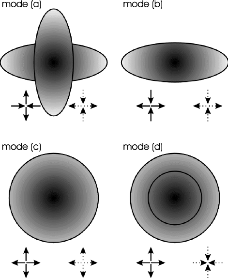
FIG. 1.: Diagrammatical representation in the $x$-$y$-plane of the four collective excitations with the lowest energy. Oscillations of particles in state $|1\rangle$ are visualized by solid line arrows, oscillations of particles in state $|2\rangle$ by dashed line arrows.

The order in which these motions appear with increasing energy depends strongly on the values of the scattering lengths involved. In Fig. 2 we display the spectrum for a positive value of $a_{11}$. For large, negative values of $a_{12}$, the two modes with the lowest energies are those with the maximum spatial overlap, namely mode $b$ and mode $c$. If we now consider the region where $a_{12}$ is positive and large, we naturally find that the modes $a$ and $d$, for which the spatial overlap is minimized, are the lowest energy modes. The point at which this crossing happens changes with changing values of $a_{11}$. Again we find, as in [14], that the widths of the condensates remain finite up to the point of collapse.

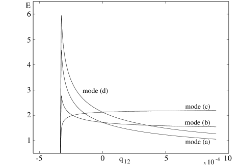
FIG. 2.: Spectrum of the low lying excitation frequencies for a fixed, positive value $q_{11}=2.3\times 10^{-4}$. With $q_{12}$ increasing from negative values to positive ones the two low lying modes and the two high lying ones get exchanged.

The eigenfrequencies (III C) provide the stability region of the equilibrium points (35),

$$N(q_{11}+q_{12}) = -\frac{4}{5}\left(\frac{1}{5}\right)^{\frac{1}{4}}$$ (42)

$$-\left(\frac{5}{4}\right)^{5}N^{4}q_{11}^{5}+\frac{1}{4}q_{11} = q_{12}.$$ (43)

Since for $a_{12}=0$ we recover the single component results [14] where only particles in one state are present, we see that for positive values of $a_{12}$ the region of stability increases and for negative ones it decreases. This is due to contributions to the total system energy from either the repulsive or attractive interaction. However, this effect is non-linear due to the nature of this interaction. It is illustrated in Fig. 3.

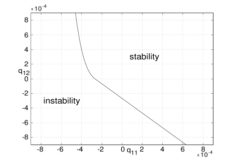
FIG. 3.: Phase diagram for the stability of the two-condensate system for $N=2000$ particles. For positive $a_{12}$ the region of stability is increased due to the positive energy contribution from the repulsive interaction. However, it does not expand linearly with increasing $a_{12}$.

IV isotropic traps and identical condensates: displaced trap centers

A Equations

Let us now consider the case of two spatially displaced traps and work out the differences to the above situation. We assume a displacement in the $x$-direction and make an ansatz analogous to Eqs.(5) and (II A) where one condensate is centered at $x_{1}=0$ and the second at $x_{2}=\alpha$. Also in this case we assume that the number of particles is conserved, what implies that the imaginary parts of the coupling constants are again zero. We apply the moment method as in the previous case and arrive, since the spatial symmetry is now broken in the $x$-direction, at the following set of equations of motion for the widths of the two condensates in the $x$-direction, $\text{w}_{nx}$, and in the $y$- and $z$-directions, $\text{w}_{n}$

$$\ddot{\text{w}}_{1x} = -\text{w}_{1x}\lambda_{1x}^{2}+\frac{1}{\text{w}_{1x}^{3}}+\frac{N_{1}q_{11}}{\text{w}_{1x}^{2}\text{w}_{1}^{2}}$$ (46)

$$+2\sqrt{8}N_{2}\frac{q_{12}\text{w}_{1x}(\text{w}_{1x}^{2}+\text{w}_{2x}^{2}-2\alpha^{2})}{(\text{w}_{1x}^{2}+\text{w}_{2x}^{2})^{\frac{5}{2}}(\text{w}_{1}^{2}+\text{w}_{2}^{2})}e^{-\frac{\alpha^{2}}{\text{w}_{1x}^{2}+\text{w}_{2x}^{2}}}$$

$$\ddot{\text{w}}_{1} = -\text{w}_{1}\lambda_{1}^{2}+\frac{1}{\text{w}_{1}^{3}}+\frac{N_{1}q_{11}}{\text{w}_{1x}\text{w}_{1}^{3}}$$ (48)

$$+2\sqrt{8}N_{2}\frac{q_{12}\text{w}_{1}}{(\text{w}_{1x}^{2}+\text{w}_{2x}^{2})^{\frac{1}{2}}(\text{w}_{1}^{2}+\text{w}_{2}^{2})^{2}}e^{-\frac{\alpha^{2}}{\text{w}_{1x}^{2}+\text{w}_{2x}^{2}}}.$$

Again one gets the equations for $\text{w}_{2x}$ and $\text{w}_{2}$ by simply exchanging the indices. We can also like, in the non-displaced case, find a potential of the form of Eq.(33), which is suitable for the derivation of these equations. However, in this case the term originating from the interaction of the particles in the different states is multiplied by an additional factor, $\exp[-\alpha^{2}/(\text{w}_{1x}^{2}+\text{w}_{2x}^{2})]$, which ensures that the influence of these interactions gets weaker, the more the condensates are displaced. This then implies an even smaller region of spatial overlap. Note that the widths of the condensates are included in this factor and it therefore has a non-negligible effect on the physics of the system in addition to weakening the magnitude of effects found in the non-displaced case.
Let us start calculating the equilibrium states for this case from Eqs.(IV A). In Fig. 4 we plotted the widths $\text{w}_{x}$ and w of the condensates for $a_{11}$ and $a_{12}$ positive and equal. Once the condensates are separated by a distance $\alpha=\sqrt{(\text{w}_{1x}^{2}+\text{w}_{2x})/2}$ the repulsive interaction between particles from different states becomes an effectively attractive one (and v.v.), as can be seen from the fact that the width on the $x$-direction gets smaller then the width in the $y$- and $z$-direction. The explanation for this effect is, that the direction of the repulsive force with respect to the surfaces of the condensates changes in these regions where they do no longer overlap. At large distances when the interaction between the particles in different states becomes negligible again, the case of two independent, isotropic condensates is recovered again.

FIG. 4.: Width of the condensates in the $x$-direction and in the $y$-,$z$-directions for $q_{11}=0.2\times 10^{4}$ and $q_{12}=0.2\times 10^{4}$. Due to the repulsive interaction between particles from different states, the condensate gets squeezed in the $x$-direction at a certain distance and then expands once the region of overlap diminishes further.

B Low energy eigenmodes and Stability

Looking at the excitation spectrum of the two component system by analyzing it again via a linear expansion around the equilibrium points, we find, as can be seen from Fig. 5, that the degeneracies existing in the non-displaced case get lifted with increasing distance. Bringing the condensates that far from each other that they can be considered as two independent condensates [14] the spectrum reduces again to two three-fold degenerate values, since the condensates become again isotropic.

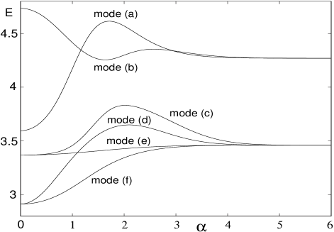
FIG. 5.: Spectrum of the low lying excitation energies for $q_{11}=q_{12}=6\times 10^{-4}$. The degeneracies are lifted with increasing $\alpha$ and for $\alpha>2$ it reduces to the case of two ,isotropic, single condenstates again.

In this Gaussian-ansatz we can again easily interpret these modes to be of the following types:

$$\begin{array}[]{rrrrrrrl}(&-\gamma_{a}&-1&-1&\gamma_{a}&1&1)&\hskip 14.22636pt\text{mode(a)}\\ (&\gamma_{b}&1&1&\gamma_{b}&1&1)&\hskip 14.22636pt\text{mode(b)}\\ (&\gamma_{c}&-1&-1&\gamma_{c}&-1&-1)&\hskip 14.22636pt\text{mode(c)}\\ (&-\gamma_{d}&1&1&\gamma_{d}&-1&-1)&\hskip 14.22636pt\text{mode(d)}\\ (&0&-1&1&0&-1&1)&\hskip 14.22636pt\text{mode(e)}\\ (&0&1&-1&0&-1&1)&\hskip 14.22636pt\text{mode(f)}\\ \end{array}$$ (49)

The members of these vectors represent the oscillation-amplitude in the directions $(\delta_{1x}\;\delta_{1y}\;\delta_{1z}\;\delta_{2x}\;\delta_{2y}\;\delta_{2z})$, where $\gamma_{l}\;(l=a,b,c,d)$ depends on the parameters of the system. The lifting of the degeneracies is mainly due to the fact, that the spatial displaced system is not invariant under an exchange of the variables $\text{w}_{1y}$ and $\text{w}_{1z}$ and not of $\text{w}_{2y}$ and $\text{w}_{2z}$, as can be seen from Eqs. (IV A).

Let us now look at the stability of the stationary states, which we again retrieve from the analysis of the Hessian matrix. As can be seen from Fig. 6 the further the condensates separate from each other, the weaker the effect of additional stabilization (destabilization) becomes, since it results from the repulsive (attractive) interaction between the condensates. For $\alpha\approx>1.5$ one recovers the stability condition for the case of two separate condensates.

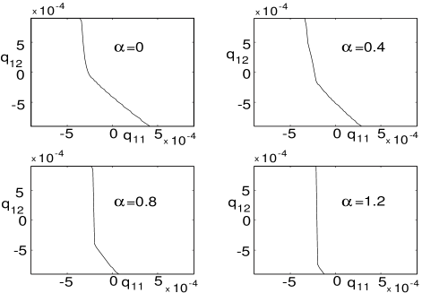
FIG. 6.: Stability region for displaced traps with a displacement parameter $\alpha$. For far displaced traps the result for independent condensates is recovered.

V conclusions

We used a moment method to describe the behavior of two overlapping Bose-Einstein-Condensates in different internal states, assuming that the shapes of the individual wave functions do not deviate too much from a Gaussian-shape. With this method it is straightforward to derive equations of motion for the open parameters defining the exact form of the Gaussian function, especially the width of the condensates. They can for the general cases easily treated numerically and for special cases even analytical solutions are possible.

For the case of isotropic traps and isotropic condensates we did calculate the equilibrium points for the system and analyzed their stability. We found, that in comparison to the case of one pure condensate the region of stability can be extended (shrinked) if the interaction energy between particles in different states is positive (negative). Due to the nonlinear character of the interaction also this effect is of nonlinear nature. It appears strongest for non-displaced traps and gets weaker the more the centers of the two traps are apart from each other. We were also able to calculate the energies of the first excited states and interpret the collective motions. For the case of displaced traps the degeneracies existing in the non-displaced case get lifted.

Acknowledgment: This work was supported by TMR network ERBFMRX-CT96-0002 and the Austrian Fond zur Förderung der wissenschaftlichen Forschung.

REFERENCES

- [1] M. H. Anderson, J. R. Ensher, M. R. Matthews, C. E. Wieman, E. A. Cornell Science, 269, 198 (1995).
- [2] C. C. Bradley, C. A. Sackett, J. J. Tollett, R. G. Hulet, Phys. Rev. Lett. 75, 1687 (1995).
- [3] K. B. Davis, M.-O. Mewes, M. R. Andrews, N. J. van Druten, D. S. Durfee, D. M. Kurn, W. Ketterle, Phys. Rev. Lett. 75, 3969 (1995).
- [4] C. J. Myatt, E. A. Burt, R. W. Ghrist, E. A. Cornell, C. E. Wieman, Phys. Rev. Lett. 78, 586 (1997)
- [5] S. N. Bose, Z. Phys. 26, 178 (1924); A. Einstein, Sitz. Preuss Akad. Wiss., 3 (1924).
- [6] M. Edwards et al., Phys. Rev. A, 53, R1950 (1996); Edwards et al., preprint;
- [7] F. Dalfovo, S. Stringari, Phys. Rev. A 53 2477 (1996)
- [8] G. Baym, C. J. Pehtick, Phys. Rev. Lett. 76 6 (1996)
- [9] B. D. Esry, Phys. Rev. A 55 1147 (1997)
- [10] L. You, W. Hoston, M. Lewenstein, Phys. Rev. A 55 R1581 (1997)
- [11] M. Holland, D. Jin, M. L. Chiofalo, J. Cooper, preprint
- [12] Y. Kagan, G. V. Shlyapnikov, J. T. M. Walraven, Phys. Rev. Lett. 76, 2670 (1996)
- [13] R. Dum, Y. Castin and J. Dalibard, unpublished
- [14] V. M. Pérez-García, H. Michinel, J. I. Cirac, M. Lewenstein, P. Zoller, Phys. Rev. Lett. 77, 5320 (1996); V. M. Pérez-García, H. Michinel, J. I. Cirac, M. Lewenstein, P. Zoller, Phys. Rev. A. (1997) (submitted)
- [15] M.-O. Mewes, M. R. Andrews, D. M. Kurn, D. S. Durfee, C. G. Townsend, W . Ketterle, Phys. Rev. Lett. 78 582 (1997)
- [16] M. R. Andrews, C. G. Townsend, H.-J. Miesner, D. S. Durfee, D. M. Kurn, W. Ketterle, Science 275 637 (1997)
- [17] H. Wallis, A. Rohrl, M. Naraschewski, A. Schenzle, Phys. Rev. A 55 (2109) 1997
- [18] M. Edwards, P. A. Ruprecht, K. Burnett, R. J. Dodd, C. W. Clark, Phys. Rev. Lett. 77 1671 (1996)
- [19] R. J. Ballagh, K. Burnett, T. F. Scott, Phys. Rev. Lett. 78 1607 (1997)
- [20] M. Bijlsma, H. T. C. Stoof, Phys. Rev. A 55 498 1997
- [21] D. Anderson, Phys. Rev. A 27, 3135 (1983); Z. Fei, V. V. Konotop, M. Peyrard, L. Vázquez, Phys. Rev. E 48 (1993) 548; A. Sánchez, A. R. Bishop,F. Domínguez-Adame, Phys. Rev. E 49 4603 (1994) ; K. O. Rasmussen, O. Bang, P.L. Christiansen, Phys. Lett. A 184 241 (1994).
- [22] Tin-Lun Ho, V.B. Shenoy, Phys. Rev. Lett. 77, 3276 (1996)
- [23] R. Graham, D. Walls, preprint cond-mat/9611111
- [24] B. D. Esry, C. H. Green, J. P. Burke Jr., J. L. Bohn, preprint;
- [25] M. Desaix, D. Anderson, M. Lisak, J. Opt. Soc. Am. B 8 2082 (1991)
- [26] A phenomenological description of losses can be incorporated by assuming complex () with negative . The real part describes elastic collisions between the particles and the imaginary part accounts for collisional losses.
- [27] In the experiment of Ref. [4] the trap is anisotropic () and since the spring constants of the traps are different for both condensate states, the centers of the traps are slightly displaced due to gravity.
- [28] Oscillations in the plane can be expressed as a superposition of and oscillations.