[

Ferromagnetism in the Hubbard model on fcc–type lattices

Abstract

The Hubbard model on fcc–type lattices is studied in the dynamical mean–field theory of infinite spatial dimensions. At intermediate interaction strength finite temperature Quantum Monte Carlo calculations yield a second order phase transition to a highly polarized, metallic ferromagnetic state. The Curie temperatures are calculated as a function of electronic density and interaction strength. A necessary condition for ferromagnetism is a density of state with large spectral weight near one of the band edges.

PACS numbers: 71.27.+a, 75.10.Lp, 75.30.Kz

]

More than 30 years ago, the Hubbard model was introduced to describe band magnetism in transition metals, in particular the ferromagnets Fe, Co and Ni [1, 2, 3]. However, for a long time it appeared to be a generic model rather for anti–ferromagnetism than for ferromagnetism. At half filling (one electron per site) on bipartite lattices antiferromagnetism emerges in both weak and strong coupling perturbational approaches and, in particular, antiferromagnetism is tractable by renormalization group methods [4]. By contrast, ferromagnetism is a non–trivial strong coupling phenomenon which cannot be investigated by any standard perturbation theory. In fact, our knowledge on the possibility of ferromagnetism in the Hubbard model is still very limited. Only in a few special cases was the Hubbard model proven to have ferromagnetic order. The first rigorous result showing a fully polarized ground state, the theorem by Nagaoka [5], is only valid for a single hole added to the half filled band in the limit of infinite on–site repulsion. In the limit of low electronic density a saturated ferromagnetic ground state has been found recently in the one dimensional Hubbard model on zigzag chains [6, 7]. Further, the existence of a ground state with net polarization has been proven for the half filled band case on bipartite lattices with asymmetry in the number of sites per sublattice [8], and in ’flat–band’ systems [9].

Due to the development of new numerical algorithms and powerful computers the problem of ferromagnetism in the Hubbard model has recently become accessible to numerical investigations of finite systems, at least in reduced dimensions $(d=1,2)$. In the presence of a next nearest neighbor hopping, polarized ground states were found very recently in $d=1$ [10] and on square lattices in the case of a van Hove singularity at the Fermi energy [11].

The rigorous and numerical results mentioned above show that the stability of ferromagnetism is intimately linked with the structure of the underlying lattice and the kinetic energy (i.e. the hopping) of the electrons. This fact has also been observed by exact variational bounds for the stability of saturated ferromagnetism [12, 13, 14, 15], and within approximative methods [16]. Generally, lattices with closed loops and with frustration of the competing antiferromagnetism (non–bipartite lattices) are expected to support ferromagnetism. Non–bipartite lattices have an asymmetric density of states (DOS) and thus a peak away from the center of the band. Indeed, it has already been observed by the inventors of the model [1, 2, 3] that a DOS with a peak near one of the band edges is favorable for ferromagnetism. Hence, the fcc lattice is expected to be a good candidate for ferromagnetism because i) it has a highly asymmetric DOS and ii) antiferromagnetism is frustrated.

Since numerical studies of finite systems would allow only very small fcc lattices, we study the Hubbard model in the dynamical mean–field theory (DMFT) which becomes exact in the limit of infinite dimensions, $d=\infty$ [17, 18]. We will show that an appropriate, non–singular kinetic energy is able to induce metallic ferromagnetism in the single band Hubbard model for intermediate values of the interaction.

In the limit $d\to\infty$, the system is reduced to a dynamical single site problem [19] equivalent to an Anderson impurity model complemented by a self–consistency condition [20, 21]. Still, it cannot be solved analytically, and to avoid further approximations we employ a finite temperature Quantum Monte Carlo method [22]. Unlike traditional mean–field theories, the DMFT takes quantum fluctuations fully into account. Spatial fluctuations are neglected – an approximation which becomes exact in the limit of large coordination number, $Z$. For the three dimensional fcc lattice we have $Z=12$. The DMFT has proven to be a powerful and reliable tool for the study of three dimensional correlated Fermi systems both for thermodynamical as well as dynamical properties [18, 23]. Spectral properties are obtained by analytic continuation of the imaginary time data using the Maximum Entropy method [24]. The solution of the self–consistent single site problem provides the local self energy $\Sigma_{\sigma n}\equiv\Sigma_{\sigma}(i\omega_{n})$ ($\omega_{n}:$ Matsubara frequencies) from which the local Green function is obtained by a Dyson equation:

$$G_{\sigma n}=\frac{1}{L}\sum_{\bf k}\frac{1}{z_{\sigma n}-\epsilon({\bf k})}=\int dE\frac{N_{0}(E)}{z_{\sigma n}-E}$$ (1)

with $z_{\sigma n}=i\omega_{n}+\mu-\Sigma_{\sigma n}$. Here, $\epsilon({\bf k})$ are the single particle energies, $N_{0}(E)$ is the non–interacting DOS, and $L$ is the number of lattice sites. Investigations of the Hubbard model on the hypercubic lattice in $d=\infty$ did not show indications for ferromagnetism for finite $U$ [18, 23], however in a recent study at $U=\infty$ a ferromagnetic instability was found within the non–crossing approximation [25].

A non–trivial generalization of the fcc lattice in $d$ dimensions [14] (see also [26]) is the set of all points with integer cubic coordinates summing up to an even integer. It is a non–bipartite Bravais lattice for any dimension $d>2$. Each point has $Z=2d(d-1)$ nearest neighbors defined by all vectors $\bf x$ which can be written in the form $\bf x=\pm\bf{e}_{i}\pm\bf{e}_{j}$, with two different cubic unit vectors $\bf{e}_{i}$ and $\bf{e}_{j}$ ($i,j=1,\cdots,d$). The energy dispersion reads

$$\epsilon({\bf k})=4t\sum_{1\leq i<j\leq d}\cos{k_{i}}\cos{k_{j}}+2t^{\prime}\sum_{i=1}^{d}\cos{2k_{i}}$$ (2)

where we allow a next nearest neighbor hopping $t^{\prime}$. In the particular case $t^{\prime}=t/2$ we find $\epsilon({\bf k})=t\;\epsilon^{2}_{hc}({\bf k})-3t$ where $\epsilon_{hc}({\bf k})$ is the energy dispersion of the hypercubic lattice. This relation leads to an inverse square–root divergency of the DOS at the lower band edge in any dimension. In the limit $d=\infty$ this divergency occurs for any $t^{\prime}$, and with the proper scaling $t=1/\sqrt{Z}$ [17] the DOS can explicitly be calculated as [14]:

$$N_{0}^{d=\infty}(E)=e^{-(1+\sqrt{2}E)/2}/\sqrt{\pi(1+\sqrt{2}E)}\;.$$ (3)

$N_{0}^{d=\infty}$ was also used by Uhrig’s [26] calculation of the single spin–flip energy of the fully polarized state. There, the ferromagnet turned out to be stable against a single spin–flip over a wide density regime.

In $d=3$ for $0<t^{\prime}<t/2$ the divergency is absent, and the DOS has a typical $\sqrt{E-E_{b}}-$behavior at the lower edge $E_{b}=\epsilon(\pi,\pi/2,0)=-4t+2t^{\prime}$. For $t^{\prime}=0$ there is a weak, logarithmic divergency at $E_{b}$. The main effect of $t^{\prime}$ on the DOS is to induce a broad peak with much spectral weight near (but not right at) the lower edge. In (3) and in the following the energy scale is set by the variance of the non–interacting DOS. In $d=3$ for $0<t^{\prime}<t/2$ the total band width is $W=16t+4t^{\prime}$. By fixing the variance of the DOS, $v=\sqrt{12t^{2}+6t^{\prime 2}}\equiv 1$, the band width ranges from 4.618 for $t^{\prime}=0$ to 4.899 for $t^{\prime}=t/2$. Comparing with real 3d–transition metals, e.g. Ni, one can roughly identify our energy scale with 1eV.

We will consider the following two cases: i) strictly $d=\infty$, i.e. using the DOS (3) and ii) $d=3$ lattices, i.e. using the DOS of the the three dimensional lattice in (1). In practice we perform finite sums over the $\bf{k}$–vectors corresponding to a finite three dimensional lattice. To keep the finite size error at least one order of magnitude smaller than the statistical errors, the number of lattice sites (respectively $\bf{k}$–vectors) has to be of the order of $10^{5}$ to $10^{7}$ depending on temperature. The computer time for this summation is still much smaller than for the Monte Carlo sampling.

To detect a ferromagnetic instability we determine the temperature dependence of the uniform static susceptibility, $\chi_{F}$, from the two particle correlation functions [27]. In addition, we calculate commensurate magnetic susceptibilities and the compressibility (charge susceptibilty). No charge instability is observed in the parameter regime under consideration.

At an intermediate interaction strength of $U=4$ we find the ferromagnetic response to be strongest around quarter filling ($n\simeq 0.5$). $\chi_{F}$ obeys a Curie–Weiss law (see Fig. 1 for case i)) and the Curie temperature $T_{c}$ can safely be extrapolated from the zero of $\chi_{F}^{-1}$ to a value of $T_{c}=0.051(2)$ at $n=0.58$ [28]. Below $T_{c}$ the magnetization $M$ grows rapidly, reaching more than 80% of the fully polarized value ($M_{max}=n=0.58$) at the lowest temperature which is only 30% below $T_{c}$. The three data points $M(T)$ (Fig. 1) are consistent with a Brillouin function with the same critical temperature of $T_{c}=0.05$ and an extrapolated full polarization at $T=0$. A saturated ground state magnetization is also consistent with the single spin–flip energy of the fully polarized state [26].

FIG. 1.: Magnetization, $M$ (diamonds), and inverse uniform static susceptibility, $\chi_{F}^{-1}$ (circles; values multiplied by a factor of 4 to use the same scale) for $U=4$ and $n=0.58$. Error–bars are of the size of the symbols or smaller. Dotted line is a linear fit to $\chi_{F}^{-1}$, dashed line a fit with a Brillouin function to $M$. (Note that the circle at $T=0.05$ is a data point, not an extrapolation.)

The Curie temperatures are obtained from the Curie–Weiss plots for different values of interaction $U$ and electronic densities $n=N_{el}/L$, leading to the phase diagram Fig. 2 for the case i). At low temperatures the system is ferromagnetic over a wide density regime. $T_{c}$ increases with $U$ and the upper critical density $n_{c}$ seems to approach $n=1$. The values of $n_{c}$ as a function of $U$ are consistent with the single spin–flip results [26]. Note that the Stoner criterion, $UN(\mu)>1$, would give $n_{c}>1$ for $U>1.5$. For low densities the Curie temperature becomes very small and seems to vanish close to $n=0$. Antiferromagnetism is not expected on the fcc lattice in high dimensions because the difference of the numbers of not frustrated bonds and frustrated bonds is only of the order of $d$ resulting in an effective field of the order of $t^{2}d\propto 1/d$ [29].

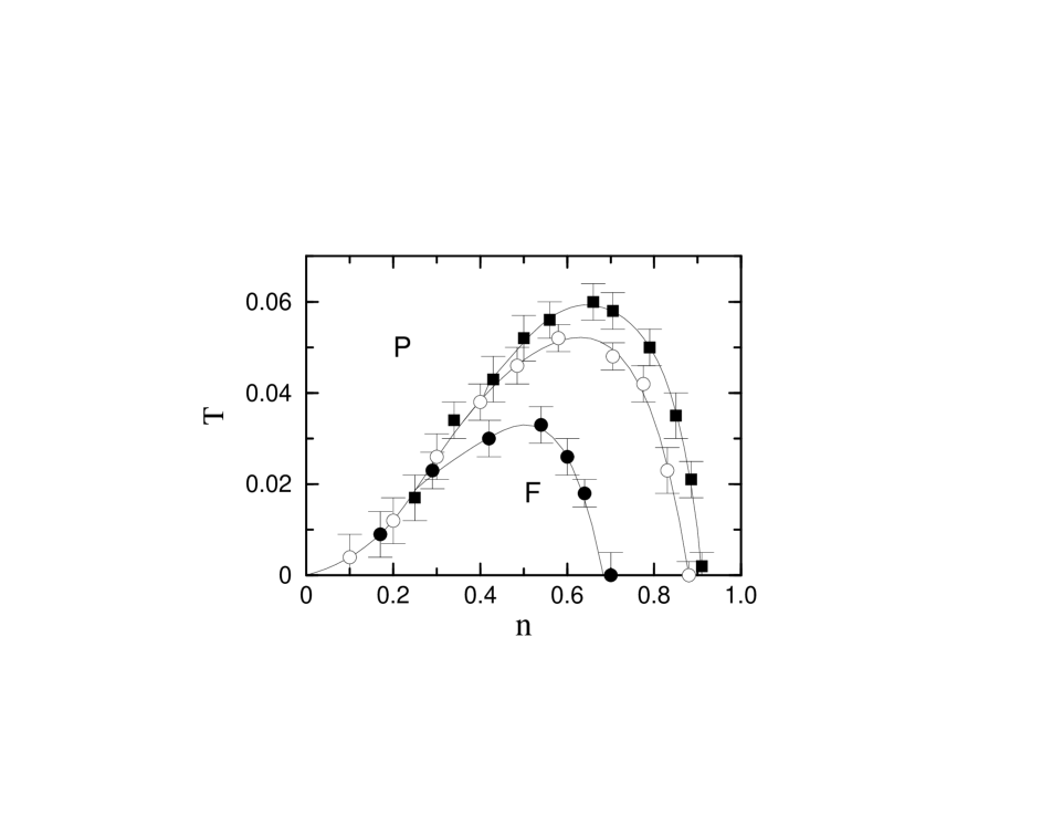
FIG. 2.: $T_{c}$ vs. $n$ phase diagram of the Hubbard model on the $d=\infty$ fcc lattice with $U=2$ (full circles), $U=4$ (open circles), and $U=5$ (squares). Lines are guides to the eye.

FIG. 3.: Phase diagram of the Hubbard model on the $d=3$ fcc lattice with $t^{\prime}=t/4$ and $U=6$. Circles: ferromagnetic, squares antiferromagnetic phase boundary.

In case ii) we first studied the pure fcc lattice, i.e. $t^{\prime}=0$. However in this situation, and for intermediate $U-$values ($U\leq 6)$ the Curie–Weiss extrapolation would lead to very small Curie temperatures, numerically indistinguishable from $T_{c}=0$. If we, however, introduce a next nearest neighbor hopping term of $t^{\prime}=t/4$ the situation is again similar to the case i). The phase diagram for $U=6$ (Fig. 3) shows a large ferromagnetic regime with an optimal density about $n=0.65$. For $U=4$ no ferromagnetism was found for temperatures accessible to the Monte Carlo technique. In contrast to the case i) now there seems to exist a finite lower critical density. This might be due to the fact that the DOS has no divergency at the band edge but a foot. An additional feature is the antiferromagnetic phase very close to half filling. We found an instability at ${\bf k}=(\pi,0,0)$, corresponding to ferromagnetic planes with alternating orientation in direction perpendicular to the planes. In addition there seem to be instabilities at ${\bf k}=(\pi/2,\pi/2,\pi/2)$ and ${\bf k}=(\pi/2,\pi/2,0)$, however only at $n=1$ and very low temperatures $(T<0.01)$. At $n=1$ the Néel temperature is (numerically) degenerate with an instability at ${\bf k}=(\pi,\pi/2,0)$. Below half filling the latter is more strongly suppressed.

The single particle spectra for spins parallel and antiparallel to the net magnetization (Fig. 4 for case i)) are apparently metallic since both spectra have a finite value at the Fermi level ($\omega=\mu$). This also holds in the paramagnetic phase (not shown). The minority spin spectrum (dotted line in Fig. 4) is not only shifted to higher frequencies but has also a little foot at low energies. This foot contains about 50% of the spectral weight below $\mu$ and looses weight with increasing polarization. The minority spin spectrum shows a pronounced upper band around $\omega-\mu\approx U=4$ with a developing (pseudo) gap. The majority spin spectrum, however, is only slightly affected by the interaction. Here, the weight of the upper band is very small since the Pauli principle makes it unlikely for the majority spin–electrons to hop over occupied sites.

FIG. 4.: Single particle spectrum, $N(\omega)$, for $U=4$, $n=0.58$, and $T=0.04$. Full (dotted) line: majority (minority) spin spectrum.

The exchange splitting, defined by the difference of the peak positions, is $\Delta\approx 0.43$ which is significantly smaller than the shift $\Delta^{Stoner}=UM\approx 2$ in Stoner theory. Further, Stoner theory would give a Curie temperature $T_{c}^{Stoner}\approx 0.5$ which is one order of magnitude too high. Thus, the mean–field Stoner theory cannot describe the different energy scales correctly. Identifying our energy scale with 1eV, the resulting Curie temperature corresponds to $T_{c}\approx 600K$. We note that this value and the large ratio $\Delta/T_{c}>8$ – which will even somewhat increase for $T\to 0$ – are in good agreement with experimental values on fcc Ni ($T_{c}=627K$, $\Delta/T_{c}\approx 10$) [30]. The agreement is quite surprising considering the neglect of band degeneracy and inter–orbital interactions favoring ferromagnetism (Hund’s coupling).

While the saturated ferromagnet has zero interaction energy ($U\langle d\rangle=0$), the mobility of the electrons and hence the kinetic energy is very poor, since electrons cannot hop over occupied sites. The paramagnetic state, on the other hand, also tries to minimize double occupancies, $\langle d\rangle$, and thus has a small kinetic energy, too. For example at $U=4$ and $n=0.58$, we find $U\langle d\rangle<0.01$ for $T<0.06$. Hence the gain in interaction energy cannot account for the relatively high Curie temperatures. This raises the question: under which circumstances has the fully polarized ferromagnet a lower kinetic energy than the paramagnet? In a one–particle picture at $T=0$ the kinetic energy difference is:

$${\Delta E}=\int^{E_{\mbox{\em Ferro}}}dE\,E\,N_{0}(E)-2\int^{E_{P}}dE\,E\,\tilde{N}(E)$$ (4)

where the Fermi levels $E_{\mbox{\em Ferro}}$ and $E_{P}$ have to determined by the density $n$. In (4), $\tilde{N}(E)$ is the (unknown) DOS of the correlated paramagnet. To get an idea of the energy difference we consider the following simple picture: since double occupancies are effectively suppressed by $U$, the band will consist of two parts separated by an energy $U$. For a given $\uparrow$–electron the average number of nearest neighbors which are not occupied by $\downarrow$–electrons is $q=1-n_{\downarrow}=1-n/2$ in the paramagnet, and hence the effective width of the lower band will be reduced by that very factor $q$. The simplest assumption for the lower part of the spectrum is $\tilde{N}(E)=N_{0}(E/q)$ i.e. a renormalization of the energies [31]. For the DOS (3), ${\Delta E}(n)$ is negative for all densities $0<n<1$ and vanishes for $n=0$ and $n=1$. The density dependence of $|{\Delta E}(n)|$ resembles strongly the $T_{c}(n)$ data (Fig. 2). In particular $|{\Delta E}(n)|$ becomes maximal at $n=0.735$ with $|{\Delta E}|_{max}=0.0747$. For a DOS with the same shape but a divergency at the upper edge, ${\Delta E}$ is always positive, i.e. the ferromagnet is totally unstable. Apparently this simple treatment of the correlated paramagnet describes qualitatively the stability of the ferromagnet depending on the structure of the non–interacting DOS, and gives even the correct energy scale for $T_{c}$. To check this approximation one can also estimate $\Delta E$ by replacing the second integral of (4) by a numerical integration over the finite temperature DOS in the paramagnetic solution. For $n=0.58$, $U=4$, and $T=0.04$ (cf. Fig. 4, but now in the paramagnetic solution) we obtain $\Delta E^{\prime}\approx-0.04(1)$ [32] which is in reasonable agreement with the simple approximation above ($\Delta E=-0.064$).

In summary, we presented a numerical proof of metallic ferromagnetism in the single band Hubbard model in the dynamical mean–field theory. A density of states with large spectral weight near one of the band edges is an essential ingredient for ferromagnetism. This condition goes far beyond the Stoner criterion, $UN_{0}(\mu)>1$, because it is the band renormalization of the interacting paramagnet – a manifest many body effect – which determines the stability of ferromagnetism.

The author acknowledges helpful discussions and correspondence with K. Held, E. Müller-Hartmann, R. Scalettar, J. Schlipf, G. Uhrig, D. Vollhardt, and J. Wahle. He thanks A. Sandvik for kindly providing his Maximum Entropy program. This work was supported in part by a grant from the ONR, N00014–93–1–0495 and by the DFG.

REFERENCES

- [1] M. C. Gutzwiller, Phys. Rev. Lett. 10, 159 (1963).
- [2] J. Hubbard, Prog. Roy. Soc. London A 276, 238 (1963).
- [3] J. Kanamori, Prog. Theor. Phys. 30, 275 (1963).
- [4] R. Shankar, Rev. Mod. Phys. 66, 129 (1994).
- [5] Y. Nagaoka, Phys. Rev. 147, 392 (1966).
- [6] E. Müller-Hartmann, J. Low. Temp. Phys. 99, 349 (1995).
- [7] For similar lattices with two minima in the dispersion ferromagnetism was found in the case of a half filled subband. H. Tasaki, Phys. Rev. Lett. 75, 4678 (1995).
- [8] E. H. Lieb, Phys. Rev. Lett. 62, 1201 (1989).
- [9] A. Mielke and H. Tasaki, Commun. Math. Phys. 158, 341 (1993).
- [10] S. Daul and R. M. Noack, Z. Phys. B 103, 293 (1997).
- [11] R. Hlubina, S. Sorella, and F. Guinea, Phys. Rev. Lett. 78, 1343 (1997).
- [12] B. S. Shastry, H. R. Krishnamurthy, and P. W. Anderson, Phys. Rev. B 41, 2375 (1990).
- [13] P. Fazekas, B. Menge, and E. Müller-Hartmann, Z. Phys. B 78, 69 (1990).
- [14] E. Müller-Hartmann, in Proc. V Symp. Phys. of Metals, edited by E. Talik and J. Szade (Poland, 1991), p. 22.
- [15] T. Hanisch, B. Kleine, A. Ritzl, and E. Müller-Hartmann, Ann. Physik 4, 303 (1995). T. Hanisch, G. Uhrig, and E. Müller-Hartmann, Phys. Rev. B 56, 13960 (1997).
- [16] T. Herrmann and W. Nolting, Solid State Commun. 103, 351 (1997); M. Potthoff, T. Herrmann, and W. Nolting, preprint.
- [17] W. Metzner and D. Vollhardt, Phys. Rev. Lett. 62, 324 (1989); D. Vollhardt, in Correlated Electron Systems, edited by V. J. Emery (World Scientific, Singapore, 1993), p. 57.
- [18] A. Georges, G. Kotliar, W. Krauth, and M. Rozenberg, Rev. Mod. Phys. 68, 13 (1996).
- [19] V. Janiš, Z. Phys. B 83, 227 (1991).
- [20] A. Georges and G. Kotliar, Phys. Rev. B 45, 6479 (1992).
- [21] M. Jarrell, Phys. Rev. Lett. 69, 168 (1992).
- [22] J. E. Hirsch and R. M. Fye, Phys. Rev. Lett. 56, 2521 (1986).
- [23] T. Pruschke, M. Jarrell, and J. K. Freericks, Adv. Phys. 44, 187 (1995).
- [24] For a review see M. Jarrell and J. E. Gubernatis, Phys. Rep. 269, 133 (1996).
- [25] T. Obermeier, T. Pruschke, and J. Keller, Phys. Rev. B 56, R8479 (1997).
- [26] G. S. Uhrig, Phys. Rev. Lett. 77, 3629 (1996).
- [27] M. Ulmke, V. Janiš, and D. Vollhardt, Phys. Rev. B 51, 10411 (1995).
- [28] The data in Fig. 1 are obtained for one small but fixed discretization in imaginary time. The error in is predominantly due to the additional extrapolation to .
- [29] E. Müller-Hartmann (private communication); Burkhard Kleine, Dissertation, University of Cologne (1995).
- [30] E. P. Wohlfarth, in Ferromagnetic Materials, Vol. 1, edited by E. P. Wohlfarth (North Holland, Amsterdam, 1980), p. 1, and references therein.
- [31] In the limit of large this turns out to be equivalent to the Hubbard-I approximation [2].
- [32] The error in is due to uncertainties in the analytic continuation and in the electronic density. The temperature broadening of the the Fermi–Dirac function is negligable at .