abbr dcu

Quantitative analysis of a Schaffer collateral model

1 Introduction

Recent advances in techniques for the formal analysis of neural networks [Ami+87, Gar88, Tso+88, Tre90, Nad+93] have introduced the possibility of detailed quantitative analyses of real brain circuitry. This approach is particularly appropriate for regions such as the hippocampus, which show distinct structure and for which the microanatomy is relatively simple and well known.

The hippocampus, as archicortex, is thought to pre-date phylogenetically the more complex neocortex, and certainly possesses a simplified version of the six-layered neocortical stratification. It is not of interest merely because of its simplicity, however: evidence from numerous experimental paradigms and species points to a prominent role in the formation of long-term memory, one of the core problems of cognitive neuroscience [Sco+57, Wei87, Gaf92, Coh+93, McN+87, Rol91]. Much useful research in neurophysiology and neuropsychology has been directed qualitatively, and even merely categorially, at understanding hippocampal function. Awareness has dawned, however, that the analysis of quantitative aspects of hippocampal organisation is essential to an understanding of why evolutionary pressures have resulted in the mammalian hippocampal system being the way it is [Ama+90, Tre+96, Ste83, Wit+92]. Such an understanding will require a theoretical framework (or formalism) that is sufficiently powerful to yield quantitative expressions for meaningful parameters, that can be considered valid for the real hippocampus, is parsimonious with known physiology, and is simple enough to avoid being swamped by details that might obscure phenomena of real interest.

The foundations of at least one such formalism were laid with the notion that the recurrent collateral connections of subregion CA3 of the hippocampus allow it to function as an autoassociative memory (Rol89, 1989, although many of the ideas go back to Mar71, 1971), and with subsequent quantitative analysis (reviewed in Tre+94, 1994). After the laying of foundations, it is important to begin erecting a structural framework. In this context, this refers to the modelling of further features of the hippocampal system, in a parsimonious and simplistic way. Tre95 introduced a model of the Schaffer collaterals, the axonal projections which reach from the CA3 pyramidal cells into subregion CA1, forming a major part of the output from CA3 and of the input to CA1. The Schaffer collaterals can be seen clearly in Figure 1, a schematic drawing of the hippocampal formation. This paper introduced an information theoretic formalism similar to that of Nad+93 to the analysis. As will become apparent, this approach to network analysis appears to be particularly powerful, and is certain to find diverse application in the future.

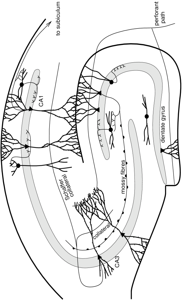
Figure 1: A schematic diagram of the hippocampal formation. Information enters the hippocampus from layer 2 entorhinal cells by the perforant path, which projects into dentate gyrus, CA3 and CA1 areas. In addition to its perforant path inputs, CA3 receives a lesser number of mossy fibre synapses from the dentate granule cells. The axons of the CA3 pyramidal cells project commissurally, recurrently within CA3, and also forward to area CA1 by the Schaffer collateral pathway. Information leaves the hippocampus via backprojections to the entorhinal cortex from CA1 and the subiculum, and also via the fornix to the mammillary bodies and anterior nucleus of the thalamus.

Once the rudiments of a structural framework have been erected, it is possible to begin to add to the fabric of the theory – to begin to consider the effect of additional details of biology that were not in themselves necessary to its structural basis. This is where the contribution of the work described in this chapter lies. The analysis described in [Tre95] assumed, for the purposes of simplicity of analysis, that the distribution of patterns of firing of CA3 pyramidal neurons was binary (and for one case ternary), although it considered threshold-linear (and thus analogue) model neurons. Here we shall consider in more detail the effect on information transmission of the possible graded nature of neuronal signalling. Another simple assumption made was that the pattern of convergence (the number of connections each CA1 neuron receives from CA3 neurons) of the Schaffer collaterals was either uniform, or alternatively bi-layered. The real situation is slightly more complex, and a better approximation of it is considered here.

2 A model of the Schaffer collaterals

The Schaffer collateral model describes, in a simplified form, the connections from the $N$ CA3 pyramidal cells to the $M$ CA1 pyramidal cells. Most Schaffer collateral axons project into the stratum radiatum of CA1, although CA3 neurons proximal to CA1 tend to project into the stratum oriens [Ish+90]; in the model these are assumed to have the same effect on the recipient pyramidal cells. Inhibitory interneurons are considered to act only as regulators of pyramidal cell activity. The perforant path synapses to CA1 cells are at this stage ignored (although they have been considered elsewhere; see Ful+96, this volume), as are the few CA1 recurrent collaterals. The system is considered for the purpose of analysis to operate in two distinct modes: storage and retrieval. During storage the Schaffer collateral synaptic efficacies are modified using a Hebbian rule reflecting the conjunction of pre- and post-synaptic activity. This modification has a slower time-constant than that governing neuronal activity, and thus does not affect the current CA1 output. During retrieval the Schaffer collaterals relay a pattern of neural firing with synaptic efficacies which reflect all previous storage events. In the following, the superscript $S$ is used to indicate the storage phase, and $R$ to indicate the retrieval phase.

• $\{\eta_{i}\}$ are the firing rates of each cell $i$ of CA3. The probability density of finding a given firing pattern is taken to be:

  $$P(\{\eta_{i}\})=\prod_{i}P_{\eta}(\eta_{i})d\eta_{i}$$ (1)

  where $\eta$ is the vector of the above firing rates. This assumption means that each cell in CA3 is taken to code for independent information, an idealised version of the idea that by this stage most of the redundancy present in earlier representations has been removed.

• $\{V_{i}\}$ are the firing rates in the pattern retrieved from CA3, and they are taken to reproduce the $\{\eta_{i}\}$ with some Gaussian distortion (noise), followed by rectification

  $$V_{i} = [\eta_{i}+\delta_{i}]^{+}$$

  $$\left<(\delta_{i})^{2}\right> = \sigma^{2}_{\delta}$$ (2)

  (the rectifying function $[x]^{+}=x$ for $x>0$, and 0 otherwise, ensures that a firing rate is a positive quantity. This results in the probability density of $V_{i}$ having a point component at zero equal to the sub-zero contribution, in addition to the smooth component). $\sigma_{\delta}$ can be related (e.g.) to interference effects due to the loading of other memory patterns in CA3 (see below and Tre+91 1991). This and the following noise terms are all taken to have zero means.

• $\{\xi_{j}\}$ are the firing rates produced in each cell $j$ of CA1, during the storage of the CA3 representation; they are determined by the matrix multiplication of the pattern $\{\eta_{i}\}$ with the synaptic weights $J_{ij}$ – of zero mean, as explained below, and variance $\sigma_{J}^{2}$ – followed by Gaussian distortion, (inhibition-dependent) thresholding and rectification

  $$\xi_{j} = \left[\xi_{0}+\sum_{i}c_{ij}J^{S}_{ij}\eta_{i}+\epsilon^{S}_{j}\right]^{+}$$

  $$\left<(\epsilon^{S}_{j})^{2}\right> = \sigma^{2}_{\epsilon^{S}}$$

  $$\left<(J^{S}_{ij})^{2}\right> = \sigma^{2}_{J}.$$ (3)

  The synaptic matrix is very sparse as each CA1 cell receives inputs from only $C_{j}$ (of the order of $10^{4}$) cells in CA3. The average of $C_{j}$ across cells is with each other. denoted as $C$

  $$c_{ij} = \{0,1\}$$

  $$\left<c_{ij}\right>N = C_{j}\qquad(C\equiv\left<C_{j}\right>)$$ (4)

• $\{U_{j}\}$ are the firing rates produced in CA1 by the pattern $\{V_{i}\}$ retrieved in CA3

  $$U_{j} = \left[U_{0}+\sum_{i}c_{ij}J^{R}_{ij}V_{i}+\epsilon^{R}_{j}\right]^{+}$$

  $$\left<(\epsilon^{R}_{j})^{2}\right> = \sigma^{2}_{\epsilon^{R}}$$

  $$\left<(J^{R}_{ij})^{2}\right> = \sigma^{2}_{J}$$ (5)

  Each weight of the synaptic matrix during retrieval of a specific pattern,

  $$J^{R}_{ij}=\cos(\theta_{\mu})J^{S}_{ij}+\gamma^{1/2}(\theta_{\mu})H(\eta_{i},\xi_{j})+\sin(\theta_{\mu})J^{N}_{ij}$$ (6)

  consists of

  1. the original weight during storage, $J^{S}_{ij}$, damped by a factor $cos(\theta_{\mu})$, where $0<\theta_{\mu}<\pi/2$ parameterises the time elapsed between the storage and retrieval of pattern $\mu$ ($\mu$ is a shorthand for the pattern quadruplet $\{\eta_{i},V_{i},\xi_{j},U_{j}\}$ ).

  2. the modification due to the storage of $\mu$ itself, represented by a Hebbian term $H(\eta_{i},\xi_{j})$, normalised so that

     $$\left<(H(\eta,\xi))^{2}\right>=\sigma^{2}_{J};$$ (7)

     $\gamma$ measures the degree of plasticity, i.e. the mean square contribution of the modification induced by one pattern, over the overall variance, across time, of the synaptic weight.

  3. the superimposed modifications $J^{N}$ reflecting the successive storage of new intervening patterns, again normalised such that

     $$\left<(J^{N}_{ij})^{2}\right>=\sigma^{2}_{J}.$$ (8)

The mean value across all patterns of each synaptic weight is taken to be equal across synapses, and is therefore taken into the threshold term. The synaptic weights $J_{ij}^{R}$ and $J_{ij}^{S}$ are thus of zero mean, and variance $\sigma_{J}^{2}$ (all that affects the calculation is the first two moments of their distribution).

A plasticity model is used which corresponds to gradual decay of memory traces. Numbering memory patterns from $1,...,\lambda,...,\infty$ backwards, the model sets $\cos(\theta_{\lambda})$ = $exp(-\lambda\gamma_{0}/2)$ and $\gamma(\theta_{\lambda})=\gamma_{0}exp(-\lambda\gamma_{0})$. Thus the strength of older memories fades exponentially with the number of intervening memories. The same forgetting model is assumed to apply to the CA3 network, and for this network, the maximum number of patterns can be stored when the plasticity $\gamma_{0}^{CA3}=2/C$ [Tre95].

For the Hebbian term the specific form

$$H(\eta_{i},\xi_{j})={h\over\sqrt{C}}(\xi_{j}-\xi_{0})(\eta_{i}-\left<\eta_{i}\right>)$$ (9)

is used, where $h$ ensures the normalisation given in Eq. 7.

The thresholds $\xi_{0}$ and $U_{0}$ are assumed to be of fixed value in the following analysis. This need not be the case, however, and as far as the model represents (in a simplified fashion) the real hippocampus, they might be considered to be tuned to constrain the sparseness of activity in CA1 in the storage and retrieval phases of operation respectively, reflecting inhibitory control of neural activity.

The block diagram shown in Fig. 2 illustrates the relationships between the variables described in the preceding section.

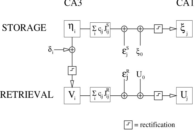
Figure 2: A block diagram illustrating the relationships between the variables present in the model. The input of the system could be considered to be the CA3 pattern during storage, $\eta$, and the output the CA1 pattern during retrieval, $U$. $J_{ij}^{R}$ depends on $J_{ij}^{S}$, $\xi_{j}$ and $\eta_{i}$ as described in the text.

3 Technical comments

The aim of the analysis is to calculate how much, on average, of the information present in the original pattern $\{\eta_{i}\}$ is still present in the effective output of the system, the pattern $\{U_{j}\}$, i.e. to average the mutual information

$$i(\{\eta_{i}\},\{U_{j}\})=\int\prod_{i}d\eta_{i}\int\prod_{j}dU_{j}P(\{\eta_{i}\},\{U_{j}\})\ln{P(\{\eta_{i}\},\{U_{j}\})\over P(\{\eta_{i}\})P(\{U_{j}\})}$$ (10)

over the variables $c_{ij},J^{S}_{ij},J^{N}_{ij}$. The details of the calculation are unfortunately too extensive to present here, and the reader will have to be satisfied with an outline of the technique used. Those not familiar with replica calculations may refer to the final chapter of [Her+91], the appendices of [Rol+97b], or, less accessibly, the book by Mez+87 for background material.

$P(\{\eta_{i}\},\{U_{j}\})$ is written (simplifying the notation) as

$$P(\eta,U)=P(U\mid\eta)P(\eta)=\int_{V}\int_{\xi}dVd\xi P(U\mid V,\xi,\eta)P(V\mid\eta)P(\xi\mid\eta)P(\eta)$$ (11)

where the probability densities implement the model defined above.

The average mutual information is evaluated using the replica trick, which amounts to

$$\log P=\lim_{n\rightarrow 0}\frac{(P^{n}-1)}{n}$$ (12)

which involves a number of subtleties, for which [Mez+87] can be consulted for a complete discussion. The important thing to note is that an assumption regarding replica symmetry is necessitated, and the stability of resulting solutions must be checked. This has been reported in [Sch+97b] for a simplified version of the neural network analysed here: a single layer of threshold-linear neurons with a single phase of operation (transmission) rather than the dual (storage and retrieval) modes in the model presented here. The conclusions of that study were that the replica-symmetric solution is stable for sufficiently sparse codes, but that for more distributed codes the solution was unstable below a critical noise variance. These conclusions can be assumed to carry across to the current model in at least a qualitative sense. In those regions (low noise, distributed codes) where the replica-symmetric solution is unstable, a solution with broken replica symmetry is required. It should be noted that it is not known what quantitative difference such a solution would bring: it may be very little, as is the case with the Hopfield network[Ami+87].

The expression for mutual information thus becomes

$$\left<i(\eta,U)\right>_{c,J^{S},J^{N}}=\lim_{n\to 0}{1\over n}\left<\int d\eta dUP(\eta,U)\left\{\left[P(\eta,U)\over P(\eta)\right]^{n}-\left[P(U)\right]^{n}\right\}\right>_{c,J^{S},J^{N}}.$$ (13)

where it is necessary to introduce $n+1$ replicas of the variables $\delta_{i},\epsilon^{S}_{j},\epsilon^{R}_{j},V_{i},\xi_{j}$ and, for the second term in curly brackets only, $\eta_{i}$.

The core of the calculation then is the calculation of the probability density $\left<P(\eta,U)^{n+1}\right>$. The key to this is “self-consistent statistics” (Rol+97b, 1997, appendix 4): all possible values of each firing rate in the system are integrated, subject to a set of constraints that implement the model. The constraints are implemented using the integral form of the Dirac $\delta$-function. Another set of Lagrange multipliers introduces macroscopic parameters

$$x^{\alpha} = \frac{1}{N}\sum_{i}\frac{(\eta_{i}^{\alpha}-\left<\eta\right>)}{\left<\eta\right>}V_{i}^{\alpha}\theta(V_{i}^{\alpha})$$

$$w^{\alpha\beta} = \frac{1}{N}\sum_{i}\eta_{i}^{\alpha}V_{i}^{\beta}\theta(V_{i}^{\beta})$$

$$y^{\alpha\beta} = \frac{1}{N}\sum_{i}V_{i}^{\alpha}V_{i}^{\beta}\theta(V_{i}^{\alpha})\theta(V_{i}^{\beta})$$

$$z^{\alpha\beta} = \frac{1}{N}\sum_{i}\eta_{i}^{\alpha}\eta_{i}^{\beta}$$

where $\theta(x)$ is the Heaviside function, and $\alpha,\beta$ are replica indices. Making the assumption of replica symmetry, and performing the integrals over all microscopic parameters, with some algebra an integral expression is obtained for the average mutual information per CA3 cell. This integral over the macroscopic parameters and their respective Lagrange multipliers is evaluated using the saddle-point approximation, which is exact in the limit of an infinite number of neurons (see, for example, Jef+72, 1972) to yield the expression given in Appendix A; the saddle-points of the expression must in general be found numerically.

4 How graded is information representation on the Schaffer collaterals?

Specification of the probability density $P(\eta)$ allows different distributions of firing rates in CA3 to be considered in the analysis. Clearly the distribution of firing rates that should be considered in the analysis is that of the firing of CA3 pyramidal cells, computed over the time-constant of storage (which we can assume to be the time-constant of LTP), during only those periods where biophysical conditions are appropriate for learning to occur. Unfortunately this last caveat makes a simple fit of the firing-rate distribution from single-unit recordings fairly meaningless unless the correct assumptions regarding exactly what these conditions are in-vivo can be made. It would be fair to assume that cholinergic modulatory activity is a pre-requisite, and unfortunately we cannot know directly from single-unit recordings from the hippocampus when the cells recorded from are receiving significant cholinergic modulation. Note that it might be possible to discover this indirectly. In any event, possibly the most useful thing we can do for the present is to assume that the distribution of firing rates during storage is graded, sparse, and exponentially tailed. This accords with the observations of neurophysiologists [Bar+90, Rol+97b]. The easiest way to introduce this to the current investigation is by means of a discrete approximation to the exponential distribution, with extra weight given to low firing rates. This allows quantitative investigation of the effects of analogue resolution on the information transmission capabilities of the Schaffer collateral model.

The required CA3 firing rate distributions were formed by the mixture of the unitary distribution and the discretised exponential, using as mixture parameters the offset $\epsilon$ between their origins, and relative weightings. The distributions were constrained to have first and second moments $\left<\eta\right>$, $\left<\eta^{2}\right>,$ and thus sparseness $\left<\eta\right>^{2}/\left<\eta^{2}\right>$, equal to $a$. In the cases considered here, $a$ was allowed values of 0.05, 0.10 and 0.20 only. The width of the distribution examined was set to 3.0, and the number of discretised firing levels contained in this width parameterised as $l$. The binary distribution was completely specified by this; for distributions with a large number of levels, there was some degree of freedom, but its numerical effect on the resulting distributions was essentially negligible. Those distributions with a small number of levels $\geq 2$ were non-unique, and were chosen fairly arbitrarily for the following results, as those that had entropies interpolating between the binary and large $l$ situations. Some examples of the distributions used are shown in Fig. 3a.

a

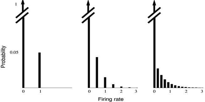
b

c

d

e

Figure 3: a Some of the CA3 firing rate distributions used in the analysis. These are, in general, formed by the mixture of a unitary distribution and a discretised exponential. b – d The mutual information between patterns of firing in CA1 and patterns of firing in CA3, expressed in natural units (nats). Asterisks represent the entropy of the CA3 pattern distribution, diamonds the CA1 retrieved mutual information, and crosses the CA1 information during the storage phase. The horizontal axis parameterises the number of discrete levels in the input distribution: for codes with fine analogue resolution, this is greater. b is for $a=0.05$ (sparse), c for $a=0.10$, and d for $a=0.20$ (slightly more distributed). e The dependence of information transmission on the degree of plasticity in the Schaffer collaterals, for $a=0.05$ (solid) and $a=0.10$ (dashed). A binary pattern distribution was used in this case.

The total entropy per cell of the CA3 firing pattern, given a probability distribution characterised by $L$ levels, is

$$h(\eta)=-\sum_{l=1}^{L}P_{\eta_{l}}(\eta_{l})\ln P_{\eta_{l}}(\eta_{l}).$$ (15)

The results are shown in Fig. 3b–d. The entropy present in the CA3 firing rate distributions is marked by asterisks. The mutual information conveyed by the retrieved pattern of CA1 firing rates, which must be strictly less than the CA3 entropy, is represented by circles. It is apparent that maximum information efficiency occurs in the binary limit. More remarkably, even in absolute terms the information conveyed is maximal for low resolution codes, at least for quite sparse codes. The results are qualitatively consistent over sparsenesses $a$ ranging from 0.05 to 0.2; obviously with higher $a$ (more distributed codes), entropies are greater. For more distributed codes (i.e. with signalling more evenly distributed over neuronal firing rates), it appears that there may be some small absolute increase in information with the use of analogue signalling levels.

For comparison, the crosses in the figures show the information stored in CA1. This was computed using a simpler version of the calculation, in which the mutual information $i(\{\eta_{i}\},\{\xi_{j}\})$ was calculated. Obviously, in this calculation, the CA3 and CA1 retrieval noises $\sigma_{\delta}$ and $\sigma_{\epsilon}^{R}$ are not present; on the other hand, neither is the Schaffer collateral memory term. Since the retrieved CA1 information is in every case higher than that stored, we can conclude that for the parameters considered, the additional Schaffer memory effect outweighs the deleterious effects of the retrieval noise distributions.

It follows from the forgetting model defined by Eq. 6, that information transmission is maximal when the plasticity (mean square contribution of the modification induced by one pattern) is matched in the CA3 recurrent collaterals and the Schaffer collaterals [Tre95]. It can be seen in Fig. 3e that this effect is robust to the use of more distributed patterns.

5 Non-uniform Convergence

It is assumed in [Tre95] that there is uniform convergence of connections from CA3 to CA1 across the extent of the CA1 subfield. In reality, each CA1 pyramidal neuron does not receive the same number of connections from CA3: this quantity varies across the transverse extent of CA1 (although this transverse variance may be less than that within CA3; Ama+90 1990). Ber+94 (1994) investigated this with a connectivity model constructed by simulating a Phaseolus vulgaris leucoagglutinin labelling experiment, matched to the available anatomical data. Their conclusion was that mid CA1 neurons receive more connections (8000) than those in proximal and distal CA1 (6500). The precise numbers are not important here; what is of interest is to consider the effect on information transmission of this spread in the convergence parameter $C_{j}$ about its mean $C$.

In this analysis $\sigma_{J}^{2}$ is set to $1/C$ for all cells in the network. $C$ is set using the assumption of parabolic dependence of $C_{j}$ upon transverse extent, on the basis of Fig. 5 of [Ber+94]. In order to facilitate comparison with the results reported in Tre95, $C$ is held at 10,000 for all results in this section. The model used (which we will refer to as the ‘realistic convergence’ model) is thus simply a scaled version of that due to Ber+94, with $C_{j}=7,143$ at the proximal and distal edges of CA1, and $C_{j}=11,429$ at the midpoint. Note that this refers to the number of CA3 cells contacting each CA1 cell; each may do so via more than one synapse.

The saddle-point expression (16) was evaluated numerically while varying the plasticity of the Schaffer connections, to give the relationships shown in Fig. 4a between mutual information and $\gamma_{0}^{CA1}$. The information is expressed in the figure as a fraction of the information present when the pattern is stored in CA3 (15).

a

b

Figure 4: Information transmitted as a function of Schaffer collateral plasticity. a Binary CA3 firing rate distributions. The solid line indicates the result for the realistic convergence model. The dashed lines indicate, in ascending order: (i) uniform convergence, (ii) two-tier convergence model with $C_{j}\in\{5000,15000\}$, (iii) two-tier convergence model with $C_{j}\in\{2000,18000\}$. b With more realistic CA3 firing-rate distributions (the 10-level discrete exponential approximation from the previous section). The solid line indicates the result for uniform connectivity, and the dashed line the two-tier convergence model with $C_{j}\in\{5000,15000\}$.

Two phenomena can be seen in the results. The first, as mentioned in the previous section (and discussed at more length in Tre95, 1995), is that information transmission is maximal when the plasticity of the Schaffer collaterals is approximately matched with that of the preceding stage of information processing. The second phenomenon is the increase in information throughput with spread in the convergence about its mean. This is an effect which is not immediately intuitive: it means that the increase in mutual information provided by those CA1 neurons with a greater number of connections than the mean more than compensates for the decrease in those with less than the mean. It must be remembered that what is being computed is the information provided by all CA1 cells about patterns of activity in CA3. This increase in information is a network effect that has no counterpart in the information a single CA1 cell could convey. In any case, the effect is rather small: the realistic convergence model allows the transmission of only marginally more information than the uniform model. The uniform convergence approximation might be viewed as a reasonable one for future analyses, then.

Fig. 4b shows that the situation for graded pattern distributions is almost identical. The numerical fraction of information transmitted is of course lower (but total transmitted information is similar – see previous section). The uniform and two-tier convergence models provide bounds between which the realistic case must lie.

6 Discussion and summary

This chapter examined quantitatively the effect of analogue coding resolution on the total amount of information that can be transmitted in a model of the Schaffer collaterals. The tools used were analytical and numerical, and the focus was upon relatively sparse codes. What can these results tell us about the actual code used to signal information in the mammalian hippocampus? In themselves, of course, they can make no definite statement. It could be that there is a very clear maximum for information transmission in using binary codes for the Schaffer collaterals, and yet external constraints, such as CA1 efferent processing, might make it more optimal overall to use analogue signalling. So results from a single component study must be viewed with duep caution. However, these results can provide a clear picture of the operating regime of the Schaffer collaterals, and that is after all a major aim of any analytical study.

The results from this paper reiterate some previously known points, and bring out others. For instance, it is very clear from Fig. 3 that, while nearly all of the information in the CA3 distribution can be transmitted using a binary code, this information fraction drops off rapidly with analogue level. The total amount of information transmitted is similar regardless of the amount of analogue level to be signalled – but this is a well known and relatively general fact, and accords with common sense intuition. However, the total amount of information that can be transmitted is only roughly constant. It appears, from this analysis, that while the total transmitted information drops off slightly with analogue level for very sparse codes, the maximum moves in the direction of more analogue levels for more evenly distributed codes. This provides some impetus for making more precise measurements of sparseness of coding in the hippocampus.

Another issue which this model allows us to address is the expansion ratio of the Schaffer collaterals, i.e. the ratio between the numbers of neurons in CA1 and CA3, $M/N$. It can be seen in Fig. 5 that an expansion ratio of 2 (a ‘typical’ biological value) is sufficient for CA1 to capture most of the information of CA3, and that while the gains for increasing this are diminishing, there is a rapid drop-off in information transmission if it is reduced by any significant amount. The actual expansion ratio for different mammalian species reported in the literature is subject to some variation, with the method of nuclear cell counts giving ratios between 1.4 (Long Evans rats) and 2.0 (humans) [Ser88], while stereological estimates range from 1.8 (Wistar rats) to 6.1 (humans) [Wes90]. It should be noted that in all these estimates, and particularly with larger brains, there is considerable error (L. Seress, personal communication). However, in all cases the Schaffer collateral model appears to operate in a regime in which there is at least the scope for efficient transfer of information.

Figure 5: The dependence of information transmission on the expansion ratio $r_{CA1,CA3}=M/N$.

Clearly it is essential to further constrain the model by fitting the parameters as sufficient neurophysiological data becomes available. As more parameters assume biologically measured values, the sensible ranges of values that as-yet unmeasured parameters can take will become clearer. It will then be possible to address further issues such as the quantitative importance of the constraint upon dendritic length (i.e. the number of synapses per neuron) upon information processing.

In summary, we have used techniques for the analysis of neural networks to quantitatively investigate the effect of a number of biological issues on information transmission by the Schaffer collaterals. We envisage that these techniques, developed further and applied in a wider context to networks in the medial temporal lobe, will yield considerable insight into the organisation of the mammalian hippocampal formation.

Appendix A. Expression from the Replica Evaluation

$$\left<i\right> = {\rm extr}_{y_{A},\tilde{y}_{A}}\Bigg{\{}\sum_{j}\Gamma(y_{A},w^{0},z^{0},C_{j},\gamma)-{N\over 2}y_{A}\tilde{y}_{A}$$ (16)

$$+N\int D\tilde{s}_{1}\left<F(\tilde{s}_{1},0,\eta,\tilde{y}_{A},0,0)\ln F(\tilde{s}_{1},0,\eta,\tilde{y}_{A},0,0)\right>_{\eta}\Bigg{\}}$$

$$- {\rm extr}_{y_{B},\tilde{y}_{B},w_{B},\tilde{w}_{B},z_{B},\tilde{z}_{B}}\Bigg{\{}\sum_{j}\Gamma(y_{B},w_{B},z_{B},C_{j},\gamma)$$

$$-{N\over 2}(y_{B}\tilde{y}_{B}+2w_{B}\tilde{w}_{B}+z_{B}\tilde{z}_{B})$$

$$+N\int D\tilde{s}_{1}D\tilde{s}_{2}\left<F(\tilde{s}_{1},\tilde{s}_{2},\eta,\tilde{y}_{B},\tilde{w}_{B},\tilde{z}_{B})\right>_{\eta}$$

$$\times\ln\left<F(\tilde{s}_{1},\tilde{s}_{2},\eta,\tilde{y}_{B},\tilde{w}_{B},\tilde{z}_{B})\right>_{\eta}\Bigg{\}}$$

where taking the extremum means evaluating each of the two terms, separately, at a saddle-point over the variables indicated. The notation is as follows. $N$ is the number of CA3 cells, whereas the sum over $j$ is over $M$ CA1 cells. $F$ is given by

$$F(\tilde{s}_{1},\tilde{s}_{2},\eta,\tilde{y},\tilde{w},\tilde{z}) = \Bigg{\{}\phi\left[{\eta+\sigma^{2}_{\delta}(\tilde{s}_{+}-\tilde{w}\eta)\over\sigma_{\delta}\sqrt{1+\sigma^{2}_{\delta}\tilde{y}}}\right]{1\over\sqrt{1+\sigma^{2}_{\delta}\tilde{y}}}$$ (17)

$$\times \exp{\left[\eta+\sigma^{2}_{\delta}(\tilde{s}_{+}-\tilde{w}\eta)\right]^{2}\over 2\sigma^{2}_{\delta}(1+\sigma^{2}_{\delta}\tilde{y})}+\phi\left[{-\eta\over\sigma_{\delta}}\right]\exp{\eta^{2}\over 2\sigma^{2}_{\delta}}\Bigg{\}}$$

$$\times \exp\left[\eta\tilde{s}_{-}-{\eta^{2}\over 2\sigma^{2}_{\delta}}(1+\sigma^{2}_{\delta}\tilde{z})\right]$$

and has to be averaged over $P_{\eta}$ and over the Gaussian variables of zero mean and unit variance $\tilde{s}_{1},\tilde{s}_{2}$.

$$Ds\equiv\frac{ds}{\sqrt{2\pi}}\exp-s^{2}/2\qquad\phi(x)\equiv\int_{-\infty}^{x}Ds.$$ (18)

$\tilde{y},\tilde{w}$ and $\tilde{z}$ are saddle-point parameters. $\tilde{s}_{+}$ and $\tilde{s}_{-}$ are linear combinations of $\tilde{s}_{1},\tilde{s}_{2}$:

$$\tilde{s}_{\pm}=\sum_{k=1}^{2}(\mp 1)^{(k-1)}\sqrt{\left[\sqrt{(\tilde{y}-\tilde{z})^{2}+4\tilde{w}^{2}}\mp(-1)^{k}(\tilde{y}-\tilde{z})\right](\tilde{y}\tilde{z}-\tilde{w}^{2})\over\left[\tilde{y}+\tilde{z}+(-1)^{k}\sqrt{(\tilde{y}-\tilde{z})^{2}+4\tilde{w}^{2}}\right]\sqrt{(\tilde{y}-\tilde{z})^{2}+4\tilde{w}^{2}}}\tilde{s}_{k}$$ (19)

in the last two lines of Eq. 16, but in the second line of Eq. 16 one has $\tilde{s}_{+}=\tilde{s}_{1}\sqrt{\tilde{y}_{A}},\tilde{s}_{-}=0$.

$\Gamma$ is effectively an entropy term for the CA1 activity distribution, given by

$$\Gamma(y,w,z,C_{j},\gamma) = \int{ds_{1}ds_{2}\over 2\pi\sqrt{\det{\bf T}_{j}^{\prime}}}\exp-(\begin{array}[]{cc}s_{1}&s_{2}\end{array}){({\bf T}_{j}^{\prime})^{-1}\over 2}\left(\begin{array}[]{c}s1\\ s2\end{array}\right)$$ (24)

$$\times\left[\int_{-\infty}^{0}dUG(U)\ln\int_{-\infty}^{0}dU^{\prime}G(U^{\prime})\right.$$

$$+\left.\int^{\infty}_{0}dUG(U)\ln G(U)\right],$$

where

$$G(U) = G(U;s_{1},s_{2},y,w,z,C_{j},\gamma)$$ (25)

$$= \phi\left[{(\xi_{0}-s_{2})(T_{yj}+2g_{j}T_{wj}+g^{2}_{j}T_{zj})+(U-U_{0}+s_{1}+g_{j}s_{2})(T_{wj}+g_{j}T_{zj})\over\sqrt{(T_{yj}T_{z_{j}}-T^{2}_{wj})(T_{yj}+2g_{j}T_{wj}+g^{2}_{j}T_{zj})}}\right]$$

$$\times{1\over\sqrt{2\pi(T_{yj}+2g_{j}T_{wj}+g^{2}_{j}T_{zj})}}\exp-{(U-U_{0}+s_{1}+g_{j}s_{2})^{2}\over 2(T_{yj}+2g_{j}T_{wj}+g^{2}_{j}T_{zj})}$$

$$+ \phi\left[{-(\xi_{0}-s_{2})T_{yj}-(U-U_{0}+s_{1}+g_{j}\xi_{0})T_{wj}\over\sqrt{(T_{yj}T_{z_{j}}-T^{2}_{wj})T_{yj}}}\right]$$

$$\times{1\over\sqrt{2\pi T_{yj}}}\exp-{(U-U_{0}+s_{1}+g_{j}\xi_{0})^{2}\over 2T_{yj}},$$

and

$$T_{yj} = \sigma^{2}_{\epsilon^{R}}+\sigma^{2}_{J}C_{j}(y^{0}-y)$$

$$T_{wj} = \sigma^{2}_{J}C_{j}(w^{0}-w)\cos(\theta)$$

$$T_{zj} = \sigma^{2}_{\epsilon^{S}}+\sigma^{2}_{J}C_{j}(z^{0}-z)$$ (26)

$${\bf T}_{j}^{\prime} = \sigma^{2}_{J}C_{j}\left(\begin{array}[]{cc}y&w\cos(\theta)\\ w\cos(\theta)&z\end{array}\right)$$ (29)

are effective noise terms.

$$g_{j}=h{C_{j}\over C}x^{0}\left<\eta\right>_{\eta}\sqrt{C\gamma(\theta)},$$ (30)

$y,w,z$ are saddle-point parameters (conjugated to $\tilde{y},\tilde{w}$ and $\tilde{z}$), and $x^{0},y^{0},w^{0},z^{0}$ are corresponding single-replica parameters fixed as

$$x^{0} = {1\over N}\sum_{i}\left<{(\eta_{i}-\left<\eta\right>_{\eta})\over\left<\eta\right>_{\eta}}V_{i}\right>$$

$$= \left<{(\eta-\left<\eta\right>_{\eta})\over\left<\eta\right>_{\eta}}\left[\eta\phi\left({\eta\over\sigma_{\delta}}\right)+{\sigma_{\delta}\over\sqrt{2\pi}}\exp-{1\over 2}\left({\eta\over\sigma_{\delta}}\right)^{2}\right]\right>_{\eta}$$

$$y^{0} = {1\over N}\sum_{i}\left<V_{i}^{2}\right>=\left<\left[\sigma_{\delta}^{2}+\eta^{2}\right]\phi\left({\eta\over\sigma_{\delta}}\right)+{\eta\sigma_{\delta}\over\sqrt{2\pi}}\exp-{1\over 2}\left({\eta\over\sigma_{\delta}}\right)^{2}\right>_{\eta}$$

$$w^{0} = {1\over N}\sum_{i}\left<\eta_{i}V_{i}\right>=\left<\eta\left[\eta\phi\left({\eta\over\sigma_{\delta}}\right)+{\sigma_{\delta}\over\sqrt{2\pi}}\exp-{1\over 2}\left({\eta\over\sigma_{\delta}}\right)^{2}\right]\right>_{\eta}$$

$$z^{0} = {1\over N}\sum_{i}\eta_{i}^{2}=\left<\eta^{2}\right>_{\eta}.$$ (31)

7 Appendix B. Parameter Values

Parameters used were, except where otherwise indicated in the text:

$\sigma_{\delta}$	0.30
$\sigma_{\epsilon}^{S}$	0.20
$\sigma_{\epsilon}^{R}$	0.20
$C$	10000
$\sigma_{J}^{2}$	0.0001
$\xi_{0}$	-0.4
$U_{0}$	-0.4
$M/N$	2.0

References

- [1] \harvarditem[Amaral et al.]Amaral, Ishizuka \harvardand Claiborne1990Ama+90 Amaral, D. G., Ishizuka, N. \harvardand Claiborne, B. \harvardyearleft1990\harvardyearright. Neurons, numbers and the hippocampal network, in J. Storm-Mathisen, J. Zimmer \harvardand O. P. Ottersen (eds), Understanding the brain through the hippocampus, Vol. 83 of Progress in Brain Research, Elsevier Science, chapter 17.
- [2] \harvarditem[Amit et al.]Amit, Gutfreund \harvardand Sompolinsky1987Ami+87 Amit, D., Gutfreund, H. \harvardand Sompolinsky, H. \harvardyearleft1987\harvardyearright. Statistical mechanics of neural networks near saturation, Ann. Phys. (N.Y.) 173: 30–67.
- [3] \harvarditem[Barnes et al.]Barnes, McNaughton, Mizumori, Leonard \harvardand Lin1990Bar+90 Barnes, C. A., McNaughton, B. L., Mizumori, S. J., Leonard, B. W. \harvardand Lin, L. H. \harvardyearleft1990\harvardyearright. Comparison of spatial and temporal characteristics of neuronal activity in sequential stages of hippocampal processing, Prog. Brain Res. 83: 287–300.
- [4] \harvarditemBernard \harvardand Wheal1994Ber+94 Bernard, C. \harvardand Wheal, H. V. \harvardyearleft1994\harvardyearright. Model of local connectivity patterns in CA3 and CA1 areas of the hippocampus, Hippocampus 4(5): 497–529.
- [5] \harvarditemCohen \harvardand Eichenbaum1993Coh+93 Cohen, N. J. \harvardand Eichenbaum, H. \harvardyearleft1993\harvardyearright. Memory, Amnesia and the Hippocampal System, MIT Press, Cambridge, MA.
- [6] \harvarditem[Fulvi-Mari et al.]Fulvi-Mari, Panzeri, Rolls \harvardand Treves1996Ful+96 Fulvi-Mari, C., Panzeri, S., Rolls, E. T. \harvardand Treves, A. \harvardyearleft1996\harvardyearright. A quantitative model of information processing in CA1, Abstracts of the Information Theory and the Brain II conference.
- [7] \harvarditemGaffan1992Gaf92 Gaffan, D. \harvardyearleft1992\harvardyearright. The role of the hippocampus-fornix-mamillary system in episodic memory, in L. R. Squire \harvardand N. Butters (eds), Neuropsychology of Memory, Guilford, New York, pp. 336–346.
- [8] \harvarditemGardner1988Gar88 Gardner, E. \harvardyearleft1988\harvardyearright. The space of interactions in neural network models, J. Phys. A: Math. Gen. 21: 257–270.
- [9] \harvarditem[Hertz et al.]Hertz, Krogh \harvardand Palmer1991Her+91 Hertz, J., Krogh, A. \harvardand Palmer, R. G. \harvardyearleft1991\harvardyearright. Introduction to the theory of neural computation, Addison-Wesley, Wokingham, U.K.
- [10] \harvarditem[Ishizuka et al.]Ishizuka, Weber \harvardand Amaral1990Ish+90 Ishizuka, N., Weber, J. \harvardand Amaral, D. G. \harvardyearleft1990\harvardyearright. Organization of intrahippocampal projections originating from CA3 pyramidal cells in the rat, J. Comp. Neurol. 295: 580–623.
- [11] \harvarditemJeffreys \harvardand Jeffreys1972Jef+72 Jeffreys, H. \harvardand Jeffreys, B. S. \harvardyearleft1972\harvardyearright. Methods of Mathematical Physics, third edn, Cambridge University Press, Cambridge, U.K.
- [12] \harvarditemMarr1971Mar71 Marr, D. \harvardyearleft1971\harvardyearright. Simple memory: a theory for archicortex, Phil. Trans. Roy. Soc. Lond. B262: 24–81.
- [13] \harvarditemMcNaughton \harvardand Morris1987McN+87 McNaughton, B. L. \harvardand Morris, R. G. M. \harvardyearleft1987\harvardyearright. Hippocampal synaptic enhancement and information storage within a distributed memory system, Trends Neurosci. 10: 408–415.
- [14] \harvarditem[Mezard et al.]Mezard, Parisi \harvardand Virasoro1987Mez+87 Mezard, M., Parisi, G. \harvardand Virasoro, M. \harvardyearleft1987\harvardyearright. Spin glass theory and beyond, World Scientific, Singapore.
- [15] \harvarditemNadal \harvardand Parga1993Nad+93 Nadal, J.-P. \harvardand Parga, N. \harvardyearleft1993\harvardyearright. Information processing by a perceptron in an unsupervised learning task, Network 4: 295–312.
- [16] \harvarditemRolls1989Rol89 Rolls, E. T. \harvardyearleft1989\harvardyearright. Functions of neuronal networks in the hippocampus and neocortex in memory, in J. H. Byrne \harvardand W. O. Berry (eds), Neural Models of Plasticity: Experimental and Theoretical Approaches, Academic Press, San Diego, pp. 240–265.
- [17] \harvarditemRolls1991Rol91 Rolls, E. T. \harvardyearleft1991\harvardyearright. Functions of the primate hippocampus in spatial and non-spatial memory, Hippocampus 1: 258–261.
- [18] \harvarditemRolls \harvardand Treves1997Rol+97b Rolls, E. T. \harvardand Treves, A. \harvardyearleft1997\harvardyearright. Neural networks and brain function, Oxford University Press, Oxford, U.K.
- [19] \harvarditemSchultz \harvardand Treves1997Sch+97b Schultz, S. \harvardand Treves, A. \harvardyearleft1997\harvardyearright. Stability of the replica-symmetric solution for the information conveyed by a neural network, submitted .
- [20] \harvarditemScoville \harvardand Milner1957Sco+57 Scoville, W. B. \harvardand Milner, B. \harvardyearleft1957\harvardyearright. Loss of recent memory after bilateral hippocampal lesions, J. Neurol. Neurosurg. Psychiatry 20: 11–21.
- [21] \harvarditemSeress1988Ser88 Seress, L. \harvardyearleft1988\harvardyearright. Interspecies comparison of the hippocampal formation shows increased emphasis on the Regio superior in the Ammon’s Horn of the human brain, J. Hirnforsch. 3: 335–340.
- [22] \harvarditemStephan1983Ste83 Stephan, H. \harvardyearleft1983\harvardyearright. Evolutionary trends in limbic structures, Neuroscience and Biobehavioral Reviews 7: 367–374.
- [23] \harvarditemTreves1990Tre90 Treves, A. \harvardyearleft1990\harvardyearright. Threshold-linear formal neurons in auto-associative nets, J. Phys. A: Math. Gen. 23: 2631–2650.
- [24] \harvarditemTreves1995Tre95 Treves, A. \harvardyearleft1995\harvardyearright. Quantitative estimate of the information relayed by the Schaffer collaterals, J. Comput. Neurosci. 2: 259–272.
- [25] \harvarditem[Treves et al.]Treves, Barnes \harvardand Rolls1996Tre+96 Treves, A., Barnes, C. A. \harvardand Rolls, E. T. \harvardyearleft1996\harvardyearright. Quantitative analysis of network models and of hippocampal data, in T. Ono, B. L. McNaughton, S. Molotchnikoff, E. T. Rolls \harvardand H. Nishijo (eds), Perception, Memory and Emotion: Frontier in Neuroscience, Elsevier, Amsterdam, chapter 37, pp. 567–579.
- [26] \harvarditemTreves \harvardand Rolls1991Tre+91 Treves, A. \harvardand Rolls, E. T. \harvardyearleft1991\harvardyearright. What determines the capacity of autoassociative memories in the brain, Network 2: 371–397.
- [27] \harvarditemTreves \harvardand Rolls1994Tre+94 Treves, A. \harvardand Rolls, E. T. \harvardyearleft1994\harvardyearright. A computational analysis of the role of the hippocampus in learning and memory, Hippocampus 4: 373–391.
- [28] \harvarditemTsodyks \harvardand Feigelman1988Tso+88 Tsodyks, M. V. \harvardand Feigelman, M. V. \harvardyearleft1988\harvardyearright. The enhanced storage capacity in neural networks with low activity level, Europhys. Lett. 6(2): 101–105.
- [29] \harvarditemWeiskrantz1987Wei87 Weiskrantz, L. \harvardyearleft1987\harvardyearright. Neuroanatomy of memory and amnesia: a case for multiple memory systems, Human Neurobiology 6: 93–105.
- [30] \harvarditemWest1990Wes90 West, M. J. \harvardyearleft1990\harvardyearright. Stereological studies of the hippocampus: a comparison of the hippocampal subdivisions of diverse species including hedgehogs, laboratory rodents, wild mice and men, in J. Storm-Mathisen, J. Zimmer \harvardand O. P. Ottersen (eds), Progress in Brain Research, Vol. 83, Elsevier Science, chapter 2, pp. 13–36.
- [31] \harvarditemWitter \harvardand Groenewegen1992Wit+92 Witter, M. P. \harvardand Groenewegen, H. J. \harvardyearleft1992\harvardyearright. Organizational principles of hippocampal connections, in M. R. Trimble \harvardand T. G. Bolwig (eds), The Temporal Lobes and the Limbic System, Wrightson Biomedical, Petersfield, U.K., chapter 3, pp. 37–60.
- [32]