The Short Range RVB State of Even Spin Ladders:
A Recurrent Variational Approach

Abstract

Using a recursive method we construct dimer and nondimer variational ansatzs of the ground state for the two-legged ladder, and compute the number of dimer coverings, the energy density and the spin correlation functions. The number of dimer coverings are given by the Fibonacci numbers for the dimer-RVB state and their generalization for the nondimer ones. Our method relies on the recurrent relations satisfied by the overlaps of the states with different lengths, which can be solved using generating functions. The recurrent relation method is applicable to other short range systems. Based on our results we make a conjecture about the bond amplitudes of the 2-ladder.

I Introduction

There is an increasing theoretical and experimental interest in systems formed by a finite number $n_{l}$ of coupled chains, currently known as ladders (for a review see [1]). Theoretical studies suggested that antiferromagnetic spin ladders should be gapped (gapless) depending on whether $n_{l}$ is an even (odd) number [2],[3],[4], [5], [6], [7],[8]. This prediction has been confirmed experimentally in compounds like (VO)₂P₂O₇ ($n_{l}=2$) [9], although some doubts has been recently casted on the ladder structure on this material [10] , SrCu₂O₃ ($n_{l}=2$) [11], Sr₂Cu₃O₅ ($n_{l}=3$), etc. Moreover, the theory also predicts that upon doping the even-$n_{l}$ ladders should become superconductors due to the pairing of holes [2],[5],[12]. The recent discovery of superconductivity in the 2-legged ladder compound Sr_0.4Ca_13.6Cu₂₄O₄₁ under high pressure [13] may perhaps constitute a confirmation of this prediction [14]. On the other hand the odd-$n_{l}$ ladders are not expected to superconduct.

Altogether the ladders fall in two different universality classes depending on the even/oddness of $n_{l}$, which in the limit $n_{l}\rightarrow\infty$ should converge to the same class. An example of this is given by the behaviour of the spin gap of the even-$n_{l}$ ladders which vanishes exponentially with $n_{l}$ [15], [16],[17].

A field theoretical characterization of these two universal classes can be obtained by mapping the spin ladders into the $1+1$ non-linear sigma model [18], [15]. The value of the coupling constant $\theta$, which multiplies the instanton number in the action, is given by $\theta=2\pi Sn_{l}$, where $S$ is the spin of the chain [19], [15], [20]. For $S=1/2$ and $n_{l}$ even one gets $\theta=0$ (mod 2$\pi$), which corresponds to a sigma model with a dynamically generated gap, while for $n_{l}$ odd one gets $\theta=\pi$ (mod 2$\pi$), which corresponds to a gapless sigma model which flows under the RG to the $SU(2)$ level 1 Wess Zumino model[21]. Thus the behaviour of ladders parallels that of the spin chains as function of the spin, as first cojectured by Haldane using precisely the mapping of the spin chains into the non-linear-sigma model [22], [23].

There is an alternative explanation of the qualitative difference between the even/odd ladders based on the RVB (Resonating Valence Bond) theory. According to the authors of ref. [7], the even-$n_{l}$ ladders are short ranged RVB systems with confinement of spin deffects, which leads to the existence of a spin gap and exponential decaying correlation functions; while the odd-$n_{l}$ ladders are long-range RVB systems with no confinement of deffects, no gap and power-law correlations. Strictely speaking, the above RVB interpretation based on the original ideas of Liang et al. [24] concerning the 2D AF-Heisenberg system, are an intuitive picture to explain the numerical results obtained using the DMRG [25] (Density Matrix Renormalization Group). It is therefore interesting to test the RVB picture using different techniques in order to confirm and get further insights into the short range nature of the even legged-ladders.

The first step in this direction is the study of the dimer-RVB state (also termed NNRVB, standing for nearest-neighbour RVB). This has already been pursued in [26],[27],[7] for $n_{l}=2$. Using the DMRG, the main conclusion of [7] is that one has to consider valence bonds between sites which are not NN (nearest-neighbours), going in that way beyond the dimer-RVB towards a short-range RVB state, whose structure has not yet been studied in detail.

From a mathematical viewpoint the dimer-RVB states are relatively easy to handle due to the work of Sutherland [28] which gives an elegant diagrammatic way of computing overlaps between the dimer states which form the dimer-RVB state. However the combinatorics of the nondimer-RVB states has not yet been worked out and their construction seems a priori a difficult task. We shall show in this paper that there is a way to circumvent the computational problem associated with short-range RVB states, which is based on the use of recurrent relations. The main idea is to build up the ground state of a ladder with $N+\nu$ rungs using the knowledge of the ground states with $N,N+1,\dots,N+\nu-1$ rungs. This is achieved by a recurrent relation (RR) which gives the ground state $|N+\nu\rangle$ in terms of the ground states $|N+\nu-1\rangle,\dots,|N\rangle$. We shall call $\nu$ the order of the recurrent relation. The “matching” of the various g.s.’s within the RR is achieved by means of a collection of $\nu$ states $|\phi_{1}\rangle,\dots|\phi_{\nu}\rangle$, which are the elementary building blocks of our method. Loosely speaking, $|\phi_{k}\rangle$ is a state which contains at least a bond of length $k$. For even-$n_{l}$ ladders, with $\xi$ a few lattice spacings, we expect an adequate description of the ground state for small values of $\nu$. The use of RR’s allow also the introduction, in a natural fashion, of variational parameters which we can determine by the standard minimization procedure of the ground state energy. The whole approach based on RR’s is analytic, powerful and rather straightforward, and we believe it represents a significant methodological improvement as compared with previous analytic approaches to the study of RVB states, which is applicable to other type of short range systems.

The organization of the paper is as follows. In section II we introduce the recurrent relations and compare the states generated by them with the conventional RVB states. In section III we deduce the RR’s for the norm of the ground state and the expectation value of the Hamiltonian. These RR’s are solved in section IV using generating functions, which allow us to obtain quite easily an analytic formula for the ground state energy density. The results of the minimization of the ground state energy respect to the variational parameters of the ansatzs corresponding to $\nu$ = 2 and 3, are presented in section V. In section VI we derive analytic expressions for the correlation length $\xi$ and give their numerical values for $\nu=$ 2 and 3. Finally in section VII we discuss our results and the perspectives of the RR method.

II RVB and RVA States

Generically, an RVB state is a linear superposition of singlets states constructed by pairing up the $N$ spins of a system into ${N\over 2}$ bonds ($N$ is even). Making an analogy with the BCS states one can think of an amplitude $h(i-j)$ of creating a bond, denoted by $(ij)$, between the sites $i$ and $j$ [29]. We shall work with bipartite lattices and such that $i$ $(j)$ belongs to the sublattice A (B). The total RVB wave funtion is given by [24],

$$|\psi\rangle_{RVB}=\sum_{i\in A,j\in B}h(i_{1}-j_{1})\cdots h(i_{N/2}-j_{N/2})\ (i_{1}j_{1})\cdots(i_{N/2}j_{N/2})$$ (1)

where the amplitudes $h(i-j)$ are all positive or zero in order to satisfy the Marshall sign rule [30]. For a dimer state $h(i-j)\neq 0$ unless $i$ and $j$ are nearest neighbours (NN). In a short-range RVB state, $h(i-j)$ decreases exponentially with the distance while in a long-range RVB state, $h(i-j)$ decays algebraically as $|i-j|^{-p}$ for some power $p$.

Let us consider the RVB state (1) for the two-leg ladder depicted in figure 1. We have labeled the sublattice A by $k=1,2,\ldots,N$ and the sublattice B by $\bar{k}=\overline{1},\overline{2},\ldots,\overline{N}$. The general ansatz (1) only depends on the amplitudes $h_{l}$ of the bond $(k,\overline{k+l})$ for $l=0,1,\dots$. Let us consider some examples in order to get familiar with the notation, while going through the details of the formalism.

A Columnar State

Let us first assume that only $h_{0}$ is non zero. We normalize it as $h_{0}=1$. In this case the corresponding RVB state (1) for a ladder with $N$ rungs takes the simple the form,

$$|N\rangle=\prod_{k=1}^{N}(k,\overline{k})$$ (2)

This state is actually the exact ground state of the rung Hamiltonian defined by,

$$H_{\rm rung}=J^{\prime}\sum_{k=1}^{N}{\bf S}_{k}\cdot{\bf S}_{\overline{k}}$$ (3)

where the vertical coupling constant $J^{\prime}$ is antiferromagnetic (i.e. $J^{\prime}>0$ ).

FIG. 1.: A two-legged ladder showing the labels corresponding to sublattices A and B.

The correlation length $\xi$ of the state (2) measured by the spin-spin correlator along the legs is exactly 0.

A trivial observation is that the states $|N+1\rangle$ and $|N\rangle$ given by eq. (2) are related by the equation,

$$|N+1\rangle=|N\rangle\otimes|\phi_{1}\rangle_{N+1}$$ (4)

where $|\phi_{1}\rangle_{N+1}$ denotes the singlet state located at the $(N+1)-$rung, namely,

$$|\phi_{1}\rangle_{N+1}=(N+1,\overline{N+1})$$ (5)

Eq.(4) is a $1^{st}$ order RR (i.e. $\nu=1$), which upon $N-1$ iterations reproduces the state (2), given the initial condition $|1\rangle=|\phi_{1}\rangle$.

B Dimer State

Let us assume that $h_{0}=1$ and $h_{1}$ are both different from zero. The variational parameter $h_{1}$ gives the amplitude of a horizontal bond in the RVB ansatz (1), i.e.

$$|N\rangle=\sum_{\overline{k}_{\alpha}}h_{1}^{n_{1}}(1,\overline{k}_{1})(2,\overline{k}_{2})\cdots(N,\overline{k}_{N})$$ (6)

where $n_{1}$ is the number of horizontal bonds. The state (6) is a linear superposition of dimer states of the form depicted in figure 2, and for this reason is called a dimer-RVB state. Observe that all the horizontal bonds come in pairs, for each horizontal bond at one leg forces the presence of a companion in front of it at the opposite leg.

FIG. 2.: A typical dimer state in a 2-legged ladder.

It is apparent that upon switching the Hamiltonian which contains the couplings along the legs of the ladder, namely

$$H_{\rm leg}=J\sum_{k=1}^{N-1}({\bf S}_{k}\cdot{\bf S}_{\overline{k+1}}+{\bf S}_{k+1}\cdot{\bf S}_{\overline{k}})$$ (7)

the dimer states (6) will become more probable than the columnar state (2) which contains only vertical rungs, and for $J=J^{\prime}$ one expects the amplitude $h_{1}$ to be close to 1. This expectation is based on the resonant mechanism that motivates the whole RVB approach [29], [31], and which is the main cause of the substantial lowering of the energy for the RVB states (see figure 3).

The key observation for our purposes is that the dimer state (6) of a ladder with open boundary conditions can be generated from a $2^{nd}$ order RR given by:

$$|N+2\rangle=|N+1\rangle\otimes|\phi_{1}\rangle_{N+2}+u\;|N\rangle\otimes|\phi_{2}\rangle_{N+1,N+2}$$ (8)

where the state denoted by $|\phi_{2}\rangle_{N+1,N+2}$ is made up of a pair of horizontal bonds located between the rungs at $(N+1,N+2)$, i.e.,

$$|\phi_{2}\rangle_{N+1,N+2}=(N+1,\overline{N+2})(N+2,\overline{N+1})$$ (9)

Comparing (6) with (8) we obtain the relation between the parameters $h_{1}$ and $u$,

$$u=h_{1}^{2}$$ (10)

FIG. 3.: The basic bond resonance mechanism for an elementary plaquette.

We refer to figure 4 for a diagrammatic selfexplanatory representation of the RR (8).

One expects the dimer state (6) to describe correctly ground states for which the correlation length is at most one.

FIG. 4.: Diagrammatic representation of the Recurrent Relation for $\nu=2$.

Fan and Ma have computed the ground state energy and the number of dimer states contained in the state $|N\rangle$ [26]. Let us call that number $F_{N}$ for reasons that will become clear below. $F_{N}$ is given by,

$$F_{N}=\frac{1}{\sqrt{5}}({\alpha}_{1}^{N+1}-{\alpha}_{2}^{N+1})$$ (11)

where $\alpha_{1,2}={1\over 2}(1\pm\sqrt{5})$. The key fact is to recognize eq.(11) as the Binet’s formula for the $N^{th}$ Fibonacci number [32]. This last result inmediately follows from the RR satisfied by $F_{N}$, as a consequence of eq.(8), namely,

$$F_{N+2}=F_{N+1}+F_{N}$$ (12)

This equation together with the initial values,

$$F_{0}=F_{1}=1$$ (13)

reproduce the well known Fibonacci sequence,

$$F_{N}=1,1,2,3,5,8,\ldots$$ (14)

Another way to arrive to this result is by counting the number of dimer states in (6). Calling $M$ the number of pairs of horizontal bonds ( $M=0,1,\ldots,[N/2]$, where $[x]$ denotes the integer part of $x$), one gets,

$$F_{N}=\sum_{M=0}^{[N/2]}\left(\begin{array}[]{c}N-M\\ M\end{array}\right)$$ (15)

This formula is well known in the theory of partitions [33].

C Nondimer States

These states are obtained whenever $h_{l}$ is non-zero for bonds connecting non NN (nearest-neigbour) states. As an example, let us assume that the non vanishing amplitudes are $h_{0}=1$, $h_{1}$ and $h_{2}$. In figure 5 we show “local” structures formed with these bonds. The number of configurations of this type increases enormously with the number of rungs. However not all of them are independent. The dimer states are all linearly independent.

FIG. 5.: A picture of several non-dimer states showing their increasing variety.

For example, the state depicted in fig. 5c) can be written as a linear combination of dimer states and the states in fig. 5a) and fig. 5b) [34] (see figure 6).

FIG. 6.: A non-dimer state as a linear combination of the 5 linearly independent states defining the $\nu=3$ Recurrent Relation.

It is clear from figures 5 that in order to generate the nondimer RVB states in full generality one has to consider RR’s with an arbitrary high order $\nu$. Thus, configurations 5a), 5b) and 5c) require a $3^{rd}$ order RR, configuration 5d) a $4^{th}$ order configuration, and so on. For physical reasons one expects $h_{2}<h_{0},h_{1}$, so that configurations 5d) and 5e) are much less probable than configurations 5a),b),c). Hence, if we restrict ourselves to these latter class of configurations we can again generate that class iteratively by means of the following RR,

$$|N+3\rangle=|N+2\rangle\otimes|\phi_{1}\rangle_{N+3}+u|N+1\rangle\otimes|\phi_{2}\rangle_{N+2,N+3}+v|N\rangle\otimes|\phi_{3}\rangle_{N+1,N+2,N+3}$$ (16)

FIG. 7.: A pictorical representation of the non-dimer state $|\phi_{3}\rangle$ defining the $\nu=3$ Recurrent Relation.

where $|\phi_{3}\rangle_{N+1,N+2,N+3}$ is pictured in figure 7 and its precise expression reads,

$$|\phi_{3}\rangle_{1,2,3}=\sqrt{{2\over 5}}[(1,\overline{2})(2,\overline{3})(3,\overline{1})+(1,\overline{3})(2,\overline{1})(3,\overline{2})]$$ (17)

The prefactor $\sqrt{{2\over 5}}$ is for normalization. The last term in (16) generates states with two horizontal bonds of type $h_{1}$ and one bond of type $h_{2}$, which follows the chess knight’s move [35] ( this kind of bonds have been recently considered in the study of the Hubbard model on $2\times 2\times 2$ and $4\times 4$ lattices in ref.[36] ). The relation between $h_{1},h_{2}$ and $v$ is given by,

$$\sqrt{\frac{2}{5}}v=h_{1}^{2}\;h_{2}$$ (18)

We have not included in $|\phi_{3}\rangle$ the configuration 5c) since it depends linearly on the remaining configurations contained in (16). In a sense eq.(16) generates recurrently the most important RVB configurations with bonds of type $h_{0}$, $h_{1}$ and $h_{2}$. The RR (16) will be used to generate all the states $|N\rangle$ with $N\geq 1$ provided we make the following formal identifications,

$$|N\rangle=\left\{\begin{array}[]{cc}1,&N=0\\ 0,&N<0\end{array}\right.$$ (19)

These are also the initial conditions of the RR (8).

The states generated recurrently from equations similar to (8) and (16) shall be called hereafter RVA states (standing for Recurrent Variational Approach), to distinguish them from the RVB states of the form (1). We have proved above that the RVA states produced by $1^{\rm st}$ and $2^{\rm nd}$ order RR’s actually coincide with RVB states, but this is not true for higher order RVA states. The main advantage in working with RVA states is that they can be treated analytically.

It is quite clear that we can perform some generalizations of the previous ideas. The general form of a RR of order $\nu$ can be written as,

$$|N+\nu\rangle=\sum_{l=1}^{\nu}u_{l}|N+\nu-l\rangle\otimes|\phi_{l}\rangle_{N+\nu-l+1,\ldots,N+\nu}$$ (20)

where $|\phi_{l}\rangle$ are normalized states which must be chosen to be linearly independent from the states generated in the previous steps, while $u_{l}$ are variational parameters.

The RR satisfied by the number, $F_{N}^{(\nu)}$, of linearly independent states generated by (20), is given by:

$$F_{N+\nu}^{(\nu)}=\sum_{l=1}^{\nu}F_{N+\nu-l}^{(\nu)}$$ (21)

subject to the initial conditions $F_{0}=1$ and $F_{N}=0$ for $N<0$. Therefore the higher order RR’s correspond to generalizations of the Fibonacci numbers. In section IV we shall get the following Binet’s formula for $F_{N}^{(\nu)}$,

$$F_{N}^{(\nu)}=\sum_{i=1}^{\nu}\prod_{j\neq i}{\alpha_{i}^{N+\nu-1}\over\alpha_{i}-\alpha_{j}}$$ (22)

where $\alpha_{i}$ are the roots of the polynomial $y^{\nu}-y^{\nu-1}-\ldots-y-1$.

III Recurrence Relations for Overlaps

In this and the following section we shall compute the value of the energy $\langle N|H|N\rangle/\langle N|N\rangle$ of the RVA states $|N\rangle$.

Let us proceed progresively and first consider the $2^{nd}$ order RR given by eq.(8). It is convenient to introduce the quantities $Z_{N}$ and $Y_{N}$ as:

$$\begin{array}[]{rl}Z_{N}=&\langle N|N\rangle\\ Y_{N}=&{}_{N}\langle\phi_{1}|\otimes\langle N-1|N\rangle\end{array}$$ (23)

Now one can easily derive the following RR’s,

$$\begin{array}[]{rl}Z_{N+2}=&Z_{N+1}+uY_{N+1}+u^{2}Z_{N}\\ Y_{N+2}=&Z_{N+1}+{u\over 2}Y_{N+1}\end{array}$$ (24)

where we have made use of the result,

$${}_{N+1}\langle\phi_{1}|\phi_{2}\rangle_{N,N+1}={1\over 2}|\phi_{1}\rangle_{N}$$ (25)

The RR’s (24) together with the initial conditions,

$$\begin{array}[]{c}Z_{0}=Z_{1}=1\\ Y_{0}=0,\ Y_{1}=1\end{array}$$ (26)

determine $Z_{N}$ and $Y_{N}$ for arbitrary values of $N$. This will be done in the next section using generating-function methods.

The Hamiltonian $H_{N}$ of a ladder with $N$ rungs, is given by

$$H_{N}=H_{\rm leg}+H_{\rm rung}$$ (27)

where $H_{\rm leg}$ and $H_{\rm rung}$ are defined in (3) and (7) respectively, The RR method applied to Hamiltonian overlaps requires the following definitions,

$$\begin{array}[]{cl}E_{N}=&\langle N|H_{N}|N\rangle\\ D_{N}=&{}_{N}\langle\phi_{1}|\otimes\langle N-1|H_{N}|N\rangle\end{array}$$ (28)

A straightforward computation using eqs. (8) and (25) leads to the following RR’s for $E_{N}$ and $D_{N}$,

$$\begin{array}[]{cl}E_{N+2}=&E_{N+1}+J^{\prime}\epsilon_{0}Z_{N+1}+u(D_{N+1}+(2J+J^{\prime})\epsilon_{0}Y_{N+1})+u^{2}(E_{N}+2J\epsilon_{0}Z_{N})\\ D_{N+2}=&E_{N+1}+J^{\prime}\epsilon_{0}Z_{N+1}+{u\over 2}(D_{N+1}+(2J+J^{\prime})\epsilon_{0}Y_{N+1})\end{array}$$ (29)

where $\epsilon_{0}=-3/4$ is the lowest eigenvalue of the operator ${\bf S}_{1}\cdot{\bf S}_{2}$.

The initial conditions for $E_{N}$ and $D_{N}$ are,

$$\begin{array}[]{c}E_{0}=0,\ E_{1}=J^{\prime}\epsilon_{0}\\ D_{0}=0,\ D_{1}=J^{\prime}\epsilon_{0}\end{array}$$ (30)

Before showing the power of the RR method by computing the values of several physical quantities, we set off for the generalization of equations (23) and (28) to arbitrary values of the order $\nu$ of the RR. Let us define the following quantities:

$$\begin{array}[]{lc}Z_{N,l}=_{N,\ldots,N-l+1}\langle\phi_{l}|\otimes\langle N-l|N\rangle&\\ &(l=0,1,\ldots,\nu-1)\\ E_{N,l}=_{N,\ldots,N-l+1}\langle\phi_{l}|\otimes\langle N-l|H_{N}|N\rangle&\end{array}$$ (31)

where we identify $Z_{N,0}\equiv\langle N|N\rangle$ and $E_{N,0}\equiv\langle N|H_{N}|N\rangle$.

The RR’s (20) for the ground states $|N\rangle$, does not automatically imply that the overlaps $Z_{N,l}$ also satisfy RR’s. However this is guaranteed provided the states $\{|\phi_{l}\rangle\}_{l=1}^{\nu}$ satisfy the following eqs.

$${}_{N,\ldots,N-k+1}\langle\phi_{k}|\phi_{l}\rangle_{N-l+1,\ldots,N}=\left\{\begin{array}[]{ll}\Omega_{kl}\;|\phi_{l-k}\rangle_{N-l+1,\ldots,N-k}&l>k\\ \Omega_{ll}=1&l=k\\ \Omega_{kl}\;{}_{N-l,\ldots,N-k+1}\langle\phi_{k-l}|&l<k\end{array}\right.$$ (32)

As a matter of fact, eq.(25) gives an example of conditions (32). The states $|\phi_{1}\rangle$, $|\phi_{2}\rangle$ and $|\phi_{3}\rangle$ also satisfy eqs. (32), with the overlapping matrix $\Omega$ given by,

$$\Omega^{(\nu=3)}=\left(\begin{array}[]{ccc}1&{1\over 2}&\sqrt{{2\over 5}}\\ {1\over 2}&1&\sqrt{{2\over 5}}\\ \sqrt{{2\over 5}}&\sqrt{{2\over 5}}&1\end{array}\right)$$ (33)

Eqs.(33) can be given a geometrical meaning in terms of the disentangling of connected bonds ( see figure 8).

For $\nu=3$, beside the overlaps defined in eqs.(31), we need in addition the following matrix element,

$$W_{N}=_{N}\langle\phi_{1}|\otimes_{N-1}\langle\phi_{1}|\otimes\langle N-2|N\rangle$$ (34)

The RR’s for the overlaps $Z_{N,l}(l=0,1,2)$ and $W_{N}$ can be derived from eq.(16),

$$\begin{array}[]{cl}Z_{N+3}=&Z_{N+2}+u^{2}Z_{N+1}+v^{2}Z_{N}+2u\Omega_{12}Z_{N+2,1}+2v\Omega_{13}Z_{N+2,2}+2uv\Omega_{23}Z_{N+1,1}\\ Z_{N+3,1}=&Z_{N+2}+u\Omega_{12}Z_{N+2,1}+v\Omega_{13}Z_{N+2,2}\\ Z_{N+3,2}=&uZ_{N+1}+\Omega_{12}Z_{N+2,1}+v\Omega_{23}Z_{N+1,1}\\ W_{N+3}=&u\Omega_{12}Z_{N+1}+Z_{N+2,1}+v\Omega_{12}\Omega_{13}Z_{N+1,1}\end{array}$$ (35)

The initial data to solve these RR’s are,

$$\begin{array}[]{llll}Z_{0}=1&Z_{0,1}=0&Z_{0,2}=0&W_{0}=0\\ Z_{1}=1&Z_{1,1}=1&Z_{1,2}=0&W_{1}=0\\ Z_{2}=1+u+u^{2}&Z_{2,1}=1+\frac{u}{2}&Z_{2,2}=\frac{1}{2}+u&W_{2}=1+\frac{u}{2}\end{array}$$ (36)

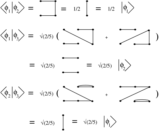
FIG. 8.: Graphical representation of the overlapping calculus for the building block states.

In order to derive RR’s for the overlaps of the Hamiltonian $H_{N}$ it is convenient to split $H_{N}$ as follows,

$$H_{N+3}=H_{N+l}+H_{N+l,N+3}$$ (37)

for different values of $l=0,1$ and 2 depending on the particular matrix elements one needs to evaluate. $H_{N+l,N+3}$ contains all the horizontal couplings between the sites $N+l$ and $N+3$ and all the vertical couplings from the rungs $N+l+1$ until $N+3$.

The analogue of eqs.(32) are now,

$$\begin{array}[]{rl}{}_{N+3,\dots,N+4-k}\langle\phi_{k}|H_{N+3-k,N+3}|\phi_{k}\rangle_{N+4-k,\dots,N+3}=&\epsilon_{kk},\,\,\,\;\;(k=1,2,3)\\ {}_{N+3}\langle\phi_{1}|H_{N+2,N+3}|\phi_{2}\rangle_{N+2,N+3}=&\epsilon_{12}|\phi_{1}\rangle_{N+2}\\ {}_{N+3}\langle\phi_{1}|H_{N+2,N+3}|\phi_{3}\rangle_{N+1,N+2,N+3}=&\epsilon_{13}|\phi_{2}\rangle_{N+1,N+2}+\epsilon^{\prime}_{13}|\phi_{1}\rangle_{N+1}|\phi_{1}\rangle_{N+2}\\ {}_{N+3,N+2}\langle\phi_{2}|H_{N+1,N+3}|\phi_{3}\rangle_{N+1,N+2,N+3}=&\epsilon_{23}|\phi_{1}\rangle_{N}\end{array}$$ (38)

together with their hermitian conjugated. The entries $\epsilon_{kl}$ can be collected into the symmetric $3\times 3$ matrix,

$$\epsilon_{kl}^{(\nu=3)}=\epsilon_{0}\left(\begin{array}[]{ccccc}J^{\prime}&&J+{J^{\prime}\over 2}&&\sqrt{{2\over 5}}({2\over 3}J+J^{\prime})\\ J+{J^{\prime}\over 2}&&2J&&3\sqrt{{2\over 5}}\,J\\ \sqrt{{2\over 5}}({2\over 3}J+J^{\prime})&&3\sqrt{{2\over 5}}\,J&&{12\over 5}(J+{1\over 4}J^{\prime})\end{array}\right)$$ (39)

while

$$\epsilon^{\prime}_{13}=\epsilon_{0}\frac{2}{3}\sqrt{\frac{2}{5}}J$$ (40)

The term proportional to $\epsilon^{\prime}_{13}$ in (38) is what forces us to introduce the overlap $W_{N}$ (34).

The RR’s for the energy overlaps are given by,

$$\begin{array}[]{cl}E_{N+3}=&E_{N+2}+\epsilon_{11}Z_{N+2}+2u(\Omega_{12}E_{N+2,1}+\epsilon_{12}Z_{N+2,1})\\ &+2v(\Omega_{13}E_{N+2,2}+\epsilon_{13}Z_{N+2,2}+\epsilon^{\prime}_{13}W_{N+2})+u^{2}(E_{N+1}+\epsilon_{22}Z_{N+1})\\ &+v^{2}(E_{N}+\epsilon_{33}Z_{N})+2uv(\Omega_{23}E_{N+1,1}+\epsilon_{23}Z_{N+1,1})\\ E_{N+3,1}=&E_{N+2}+\epsilon_{11}Z_{N+2}+u(\Omega_{12}E_{N+2,1}+\epsilon_{12}Z_{N+2,1})\\ &+v(\Omega_{13}E_{N+2,2}+\epsilon_{13}Z_{N+2,2}+{\epsilon^{\prime}}_{13}W_{N+2}\\ E_{N+3,2}=&\Omega_{12}E_{N+2,1}+\epsilon_{12}Z_{N+2,1}+u(E_{N+1}+\epsilon_{22}Z_{N+1})+v(\Omega_{23}E_{N+1,1}+\epsilon_{23}Z_{N+1,1})\end{array}$$ (41)

The initial data for the energy overlaps are

$$\begin{array}[]{lll}E_{0}=0&E_{0,1}=0&E_{0,2}=0\\ E_{1}=\epsilon_{0}J^{\prime}&E_{1,1}=\epsilon_{0}J^{\prime}&E_{1,2}=0\\ E_{2}=2\epsilon_{0}[J^{\prime}+u(J+J^{\prime})+u^{2}J]&E_{2,1}=\epsilon_{0}[2J^{\prime}+u(J^{\prime}+J)]&E_{2,2}=\epsilon_{0}(J^{\prime}+J+2uJ)\end{array}$$ (42)

IV Generating Function Methods for Solving the RR’s

The simplest way to find the general term of a series defined by a RR is by introducing generating functions. Fan and Ma in [26] have also used generating functions in order to find the ground state energy of the dimer state. However in their approach they do not start from RR’s that generate ground states, and so the appearance of generating functions seems rather obscure. Our method gives a simple and straighforward derivation of their generating function methods. Let us illustrate the technique with the derivation of the Binet formula (11).

A Number of states

For this purpose let us define the following generating function,

$$F(x)=\sum_{N\geq 0}F_{N}x^{N}$$ (43)

A simple computation using (12) and (13) yields

$$F(x)={1\over 1-x-x^{2}}$$ (44)

To recover $F_{N}$ we can use countour integrals:

$$F_{N}=\oint_{C_{0}}{dx\over 2\pi i}x^{-N-1}F(x)$$ (45)

where $C_{0}$ is a countour that encloses the origin counterclockwise.

For reasons which will become clear later on, it is convenient to perform the change of variables $x=1/y$, in which case (45) becomes:

$$F_{N}=\oint_{C_{\infty}}{dy\over 2\pi i}y^{N-1}\tilde{F}(y)=\sum Res(y^{N-1}\tilde{F}(y))$$ (46)

where

$$\tilde{F}(y)\equiv F({1\over y})$$ (47)

In (46) $C_{\infty}$ is a contour around infinity which picks up all the poles of the function $\tilde{F}(y)$. In the example (44) we get,

$$\tilde{F}(y)={y^{2}\over y^{2}-y-1}$$ (48)

Noticing that $\alpha_{1,2}={1\over 2}(1\pm\sqrt{5})$ are the two roots of the equation $y^{2}-y-1=0$, we get the Binet formula (11)

We can similarly derive eq.(22) for the number $F_{N}^{(\nu)}$ of states generated by the RR of order $\nu$. The generating functions $F^{(\nu)}(x)$ and $\tilde{F}^{\nu}(y)$ are given by:

$$\begin{array}[]{cl}F^{(\nu)}(x)=&1/(1-x-x^{2}-\ldots-x^{\nu})\\ \tilde{F}^{\nu}(y)=&y^{\nu}/(y^{\nu}-y^{\nu-1}-\ldots-y-1)\end{array}$$ (49)

B Norm and Energy of the $\nu=2$ states

Let us now solve the RR’s for $Z_{N}$ and $E_{N}$ in the $\nu=2$ case. To this end we introduce the following generating functions

$$\begin{array}[]{ll}Z(x)=\sum_{N\geq 0}Z_{N}x^{N},&Y(x)=\sum_{N\geq 0}Y_{N}x^{N}\\ E(x)=\sum_{N\geq 0}E_{N}x^{N},&\ \ D(x)=\sum_{N\geq 0}D_{N}x^{N}\end{array}$$ (50)

From equations (24), (26), (29) and (30) we find

$$\begin{array}[]{rl}(1-x-x^{2}u^{2})Z(x)=&1+xuY(x)\\ (1-{xu\over 2})Y(x)=&xZ(x)\\ (1-x-x^{2}u^{2})E(x)=&\epsilon_{0}(xJ^{\prime}+2x^{2}u^{2}J)Z(x)+\epsilon_{0}xu(2J+J^{\prime})Y(x)+xuD(x)\\ (1-{xu\over 2})D(x)=&x[E(x)+\epsilon_{0}J^{\prime}Z(x)+{u\over 2}(2J+J^{\prime})\epsilon_{0}Y(x)]\end{array}$$ (51)

Then eliminating $Y(x)$ and $D(x)$ in terms of $E(x)$ and $Z(x)$ we find,

$$Z(x)=\frac{A(x)}{B(x)},\;\;E(x)=\frac{C(x)}{B(x)^{2}}$$ (52)

where $A(x),B(x)$ and $C(x)$ are polinomials of degrees $a=1,b=3,c=4$ respectively, given by

$$\begin{array}[]{rl}A(x)=&1-\frac{1}{2}xu\\ B(x)=&1-(1+{1\over 2}u)x-(u^{2}+{1\over 2}u)x^{2}+{1\over 2}x^{3}u^{3}\\ C(x)=&\epsilon_{0}\;x\;[J^{\prime}+xu(2J+J^{\prime}+2uJ)-x^{2}u^{2}({1\over 4}J^{\prime}+2uJ)+{1\over 2}x^{3}u^{4}J]\end{array}$$ (53)

We shall show below that eqs.(52) also hold for $\nu=3$, where $A,B$ and $C$ are polinomials of degrees 3, 6 and 9 respectively. For both, $\nu=2$ and 3, we have the relation,

$$a+b=c$$ (54)

We shall again make the change of variables $x=1/y$, defining the new polinomials,

$$P(y)=y^{a}A(1/y),\;Q(y)=y^{b}B(1/y),\;R(y)=y^{c}C(1/y)$$ (55)

In the large $N$ limit, $Z_{N}$ and $E_{N}$ are given by,

$$Z_{N}\sim\alpha^{N-1-a+b}\frac{P(\alpha)}{Q^{\prime}(\alpha)},\;\;\;E_{N}\sim N\alpha^{N-1+2b-c}\frac{R(\alpha)}{\alpha Q^{\prime 2}(\alpha)}$$ (56)

where $Q^{\prime}(y)=dQ(y)/dy$ and $\alpha$ denotes the biggest root of the polynomial $Q(y)$.

The density energy per site of the 2-legged ladder is finally given by,

$$e_{\infty}=\lim_{N\rightarrow\infty}\frac{1}{2N}\frac{E_{N}}{Z_{N}}=\frac{R(\alpha)}{2\alpha Q^{\prime}(\alpha)P(\alpha)}$$ (57)

where we have employed eqs.(54,56).

C Norm and Energy of the $\nu=3$ states

A feature of the $\nu=2$ and 3 RR’s for the generating functions $Z_{l}(x)$ and $E_{l}(x)$ , which we believe is valid for higher order RR’s, is that they can be written in the following compact form,

$$\begin{array}[]{ll}\sum_{m=0}^{\nu-1}K_{lm}(x)Z_{m}(x)=e_{l},&\\ &(l=0,\dots,\nu-1)\\ \sum_{m=0}^{\nu-1}K_{lm}(x)E_{m}(x)=\sum_{m=0}^{\nu-1}L_{lm}(x)Z_{m}(x),&\end{array}$$ (58)

where $(e_{0},e_{1},\dots,e_{\nu-1})=(1,0,\dots,0)$. If $K_{lm}(x)$ is an invertible matrix then the solution of these eqs. is given by,

$$Z_{l}(x)=K^{-1}_{l0},\;\;E_{l}=K^{-1}_{lm}L_{mn}K^{-1}_{n0}$$ (59)

Calling $M_{ln}$ the $(l,n)$ minor of the matrix $K_{ln}$, then eqs(59) have the generic form postulated in (52) with the identifications,

$$A(x)=M_{00},\;\;B(x)={\rm det}K(x),\;\;C(x)=M_{0k}\;L_{kl}\;M_{l0}$$ (60)

The matrices $K(x)$ and $L(x)$ for $\nu=3$ can be derived from eqs.(35) and (41) and they read,

$$K(x)=$$ (61)

$$\left(\begin{array}[]{ccccc}1-x-{u^{2}}\,{x^{2}}-{v^{2}}\,{x^{3}}&&-2ux\left(\Omega_{12}+2v{x}\Omega_{23}\right)&&-2\,v\,x\Omega_{13}\\ -x&&1-{{u\,x}\Omega_{12}}&&-\Omega_{13}\,v\,x\\ -u\,{x^{2}}&&-x\left(\Omega_{12}+\Omega_{23}\,v\,{x}\right)&&1\end{array}\right)$$ (65)

$$\frac{1}{x}\,L(x)=$$ (66)

$$\left(\begin{array}[]{ccccc}\epsilon_{11}+\epsilon_{22}xu^{2}+x^{2}v(v\epsilon_{33}++2u\Omega_{12}\epsilon^{\prime}_{13})&&2[u\epsilon_{12}+uv\epsilon_{23}x+v\epsilon^{\prime}_{13}(x+\Omega_{12}\Omega_{13}vx^{2})]&&2v\epsilon_{13}\\ \epsilon_{11}+uvx^{2}\Omega_{12}\epsilon^{\prime}_{13}&&u\epsilon_{12}+v\epsilon^{\prime}_{13}(x+\Omega_{12}\Omega_{13}vx^{2})&&v\epsilon_{13}\\ ux\epsilon_{22}&&\epsilon_{12}+vx\epsilon_{23}&&0\end{array}\right)$$ (70)

V Minimization of the Ground State Energy: Results

In the previous section we have derived a formula for the ground state energy density, eq.(57), in terms of three polinomials evaluated at the biggest root $\alpha$ of $Q(y)$. The minimization procedure consist now in looking for the minimum of $e_{\infty}$ by varying the parameter $u$ for $\nu=2$, and the parameters $u$ and $v$ for $\nu=3$. In tables 1 and 2 we show the ground state energies per site for different values of the coupling constant ratio $J/J^{\prime}$, varying through strong, intermediate and weak coupling regimes. The values $-e_{\infty}^{(2)}/J^{\prime}$ and $-e_{\infty}^{(3)}/J^{\prime}$ are those of the RVA states for $\nu=2$ and 3. The values $-e_{\infty}^{MF}/J^{\prime}$ are Mean Field values taken from [8], [37] while $-e_{\infty}^{Lan}/J^{\prime}$ are Lanzcos values taken from [4].

$J/J^{\prime}$	$u$	$-e_{\infty}^{(2)}/J^{\prime}$	$-e_{\infty}^{MF}/J^{\prime}$	$-e_{\infty}^{Lan}/J^{\prime}$
$0$	$0$	$0.375$	$0.375000$
$0.2$	$0.128521$	$0.383114$	$0.382548$
$0.4$	$0.323211$	$0.40835$	$0.405430$
$0.6$	$0.578928$	$0.44853$	$0.442424$
$0.8$	$0.87441$	$0.499295$	$0.489552$
$1$	$1.18798$	$0.556958$	$0.542848$	$0.578$
$1.25$	$1.58519$	$0.63518$	$0.614473$	$0.6687$
$1.66$	$2.21853$	$0.772172$	$0.738360$	$0.8333$
$2.5$	$3.39153$	$1.06915$	$1.002856$	$1.18$
$5$	$5.9777$	$1.99285$		$2.265$

Table 1

J/J’	$u$	$v$	$-e_{\infty}^{(3)}/J^{\prime}$	$-e_{\infty}^{MF}/J^{\prime}$	$-e_{\infty}^{Lan}/J^{\prime}$
$0$	$0$	$0$	$0.375$	$0.375000$
$0.2$	$0.105059$	$0.0200031$	$0.383195$	$0.382548$
$0.4$	$0.230463$	$0.0911438$	$0.409442$	$0.405430$
$0.6$	$0.399714$	$0.222909$	$0.45252$	$0.442424$
$0.8$	$0.626206$	$0.42656$	$0.507909$	$0.489552$
$1$	$0.91059$	$0.716812$	$0.571314$	$0.542848$	$0.578$
$1.25$	$1.34146$	$1.22022$	$0.657551$	$0.614473$	$0.6687$
$1.66$	$2.19835$	$2.41718$	$0.808438$	$0.738360$	$0.8333$
$2.5$	$4.34045$	$6.26652$	$1.13384$	$1.002856$	$1.18$
$5$	$11.2015$	$24.0891$	$2.13608$		$2.265$

Table 2

It is also possible to minimize the energy of ladders with finite length. In table 3 we show the results obtained with the $\nu=3$ ansatz at the isotropic value $J/J^{\prime}=1$. $N$ denotes the number of vertical rungs.

$N$	$u$	$v$	$-e_{N}^{(3)}/J^{\prime}$
$3$	$0.74225$	$0.624464$	$0.521564$
$4$	$0.998703$	$0.612503$	$0.533225$
$5$	$0.90358$	$0.696407$	$0.541372$
$6$	$0.921508$	$0.64184$	$0.545944$
$7$	$0.930216$	$0.667329$	$0.549671$
$8$	$0.917952$	$0.67691$	$0.552377$
$9$	$0.920783$	$0.675904$	$0.554453$

Table 3

From these results we can make the following comments

• For any value of $J/J^{\prime}$ there is always a solution which minimizes the energy. In other words, the dimer and non dimer RVA states are physical acceptable in the whole range of couplings.

• In the strong coupling regime $J/J^{\prime}<1$ the RVA states give a slightly better ground state energy than the mean field result. This later state produces rather unphysical results for $J/J^{\prime}>1$, which does not occur in our case.

• The nondimer state improves considerably the g.s. energy as compared with the dimer state, especially for $J/J^{\prime}\geq 1$. As $J/J^{\prime}$ increase the ratio $v/u$ also increases and it is greater than one for $J/J^{\prime}\sim 1.5$. Later on we shall discuss in more detail the interpretation of the values of $u$ and $v$ in the isotropic case.

• In the weak coupling limit $J/J^{\prime}>>1$ $u$ approaches asymptotically the value 15.94, while the energy density approaches - 0.379 $J$. The later value is much greater than the exact result -0.4431 given by the Bethe ansatz solution for the decoupled spin 1/2 chains. It is however curious that in the limit $J/J^{\prime}\rightarrow\infty$ the variational parameter $u$ does not go to infinity, yielding a dimer state whose energy is - 0.375 $J$. This shows once more that the resonance mechanism always lowers the energy.

VI Spin Correlation Length

The technique we have used in the previous sections to compute the g.s. energy of the RVA states can be easily extended to the evaluation of spin-spin correlators.

A Dimer state

We want to compute the correlator $\langle{\bf S}_{1}\cdot{\bf S}_{R}\rangle$ between the spin operators at the positions 1 and $R$ on the ladder ( we assume for simplicity that both sites are on the sublattice $A$). As usual we shall define two auxiliary quantities

$$\begin{array}[]{cl}g_{N}(R)=&\langle N|{\bf S}_{1}\cdot{\bf S}_{R}|N\rangle\\ f_{N}(R)=&\langle\phi_{1}|\otimes\langle N-1|{\bf S}_{1}\cdot{\bf S}_{R}|N\rangle\end{array}$$ (71)

From the RR (8) one finds,

$$\begin{array}[]{cl}g_{N+2}(R)=&g_{N+1}(R)+u^{2}g_{N}(R)+uf_{N+1}(R)\\ f_{N+2}(R)=&g_{N+1}(R)+\frac{u}{2}f_{N+1}(R)\end{array}$$ (72)

The initial conditions are given by,

$$\begin{array}[]{rl}g_{N}(R)=2f_{N}(R)=&\left\{\begin{array}[]{ll}\frac{3}{2}\left(\frac{u}{2}\right)^{R-1}&N=R\\ 0&N<R\end{array}\right.\end{array}$$ (73)

These eqs can be derived using the Sutherland’s rules [28] which imply that there is only one loop covering giving a contribution to the correlation when the spin operators are located at the two boundaries of the chain. Defining the generating functions $g(x),f(x)$ as usual we convert the RR’s (71) into,

$$\begin{array}[]{rl}(1-x-x^{2}u^{2})g(x)=&g_{R}(R)x^{R}+xuf(x)\\ (1-\frac{1}{2}xu)f(x)=&f_{R}(R)x^{R}+xg(x)\end{array}$$ (74)

Eliminating $f(x)$ we get,

$$g(x)=g_{R}(R)x^{R}/B(x)\Longrightarrow g_{N}(R)\sim\alpha^{N-R+2}g_{R}(R)/Q^{\prime}(\alpha)$$ (75)

where $\alpha$ is the biggest root of the polynomial $Q(y)$. The correlator is finally given for $R>>1$ by,

$$\langle{\bf S}_{1}\cdot{\bf S}_{R}\rangle={g_{N}(R)\over Z_{N}}\sim\frac{3}{2(\alpha-u/2)}\left(\frac{u}{2\alpha}\right)^{R-1}$$ (76)

which gives the expected exponential decaying behaviour with the distance. The correlation length is then given by the expression,

$${\rm e}^{1/\xi}=\frac{2\alpha}{u}$$ (77)

From these result we observe that ${\cal L}={\rm exp}(1/\xi)$ satisfies the cubic equation,

$$u^{3}{\cal L}^{3}-(2+u)u^{2}{\cal L}^{2}-(2+4u)u^{2}{\cal L}+4u^{3}=0$$ (78)

Setting $u=1$ in (78) we obtain the solution of ${\cal L}=4.201472$ which yields a correlation length $\xi=0.696652$. This result has been obtained before by White et al. in reference [7], [38].

FIG. 9.: The correlation length $\xi$ for the dimer state $\nu=2$ as a function of the variational parameter $u$.

The correlation length as a function of the ratio $J/J^{\prime}$ is found by replacing in (77) the value of $u$ that minimizes the g.s. energy. We collect our results in Table 4. For the isotropic case the g.s. corresponds to $u=1.18798$, which gives a the correlation length $\xi=0.737253$, which is slightly bigger than the one given above for $u=1$.

B $\nu=3$

We shall outline the main steps of the derivation of $\xi$, since they follow those of the dimer case. In particular one gets the same asymptotic behaviour $g_{N}(R)\sim\alpha^{N-R}g_{R}(R)$. The main difficulty of the nondimer case is the computation of $g_{R}(R)$. Fortunately we can apply some kind of “nested” RR method to compute this quantity. In order to do so we need the following definitions,

$$\begin{array}[]{rl}g_{R}=&\langle R|{\bf S}_{1}\cdot{\bf S}_{R}|R\rangle\\ g_{R,1}=&\langle\phi_{1}|\otimes\langle R-1|{\bf S}_{1}\cdot{\bf S}_{R}|R\rangle\\ g_{R,2}=&\langle\phi_{2}|\otimes\langle R-2|{\bf S}_{1}\cdot{\bf S}_{R}|R\rangle\\ \tilde{g}_{R,2}=&\langle\phi_{1}|\otimes\langle R-1|{\bf S}_{1}\cdot{\bf S}_{R-1}|R\rangle\end{array}$$ (79)

The RR’s satisfied by these quantities are given by,

$$\begin{array}[]{rl}g_{R+3}=&2u\Sigma_{12}\;g_{R+2,1}+2v\Sigma_{13}\;(g_{R+2,2}+\tilde{g}_{R+2,2})+2uv\Sigma_{23}\;g_{R+1,1}\\ g_{R+3,1}=&u\Sigma_{12}\;g_{R+2,1}+v\Sigma_{13}\;(g_{R+2,2}+\tilde{g}_{R+2,2})\\ g_{R+3,2}=&\Sigma_{12}\;g_{R+2,1}+v\Sigma_{23}\;g_{R+1,1}\\ \tilde{g}_{R+3,2}=&\Omega_{12}\;g_{R+2,1}+v\Sigma_{23}\;g_{R+1,1}\end{array}$$ (80)

where we have use the matching eqs.

$$\begin{array}[]{rl}{}_{2}\langle\phi_{1}|{\bf S}_{2}|\phi_{2}\rangle_{1,2}=&\Sigma_{12}\;{\bf S}_{1}|\phi_{1}\rangle_{1}\\ {}_{3}\langle\phi_{1}|{\bf S}_{3}|\phi_{3}\rangle_{1,2,3}=&\Sigma_{13}\;({\bf S}_{1}+{\bf S}_{2})|\phi_{2}\rangle_{1,2}\\ {}_{3,2}\langle\phi_{2}|{\bf S}_{3}|\phi_{3}\rangle_{1,2,3}=&\Sigma_{23}\;{\bf S}_{1}|\phi_{1}\rangle_{1}\\ {}_{3,2}\langle\phi_{2}|{\bf S}_{2}|\phi_{3}\rangle_{1,2,3}=&\Sigma_{23}\;{\bf S}_{1}|\phi_{1}\rangle_{1}\end{array}$$ (81)

with

$$\Sigma_{12}=1/2,\;\;\Sigma_{13}=\Sigma_{23}=\frac{1}{2}\sqrt{\frac{2}{5}}$$ (82)

The initial data to iterate (80) are,

$$\begin{array}[]{llll}g_{1}={3/4},&g_{1,1}={3/4},&g_{1,2}=0,&\tilde{g}_{1,2}=0\\ g_{2}={3u/4},&g_{2,1}={3u/8},&g_{2,2}=3/8,&\tilde{g}_{2,2}=\frac{3}{4}(\frac{1}{2}+u)\end{array}$$ (83)

Using generating functions we get that the asymptotic behaviour of $g_{R}$ is given by $\beta^{R}$ where $\beta$ is the highest root of the following cubic polynomial,

$$\tilde{Q}(y)=y^{3}-\Sigma_{12}uy^{2}-2v\Sigma_{12}\;\Sigma_{13}\;y-2v^{2}\Sigma_{13}\;\Sigma_{23}\;$$ (84)

Hence the correlation length $\xi$ is given by the formula,

$${\rm e}^{1/\xi}=\frac{\alpha}{\beta}$$ (85)

which contains eq.(77) as a particular case. Indeed setting $v=0$ in (84) we get $\beta=u/2$.

In table 4 we show the values of $\xi$ computed from eq.(85), for those values of $u$ and $v$ that minimizes the g.s. energy.

$J/J^{\prime}$	$\xi^{(2)}$	$\xi^{(3)}$
$0$	$0$	$0$
$0.2$	$0.348297$	$0.437166$
$0.4$	$0.471180$	$0.608323$
$0.6$	$0.577543$	$0.751286$
$0.8$	$0.665915$	$0.866958$
$1$	$0.737253$	$0.959249$
$1.25$	$0.807398$	$1.04877$
$1.66$	$0.890758$	$1.15205$
$2.5$	$0.994468$	$1.26951$
$5$	$1.121437$	$1.38532$

Table 4

Some comments are in order

• There is an improvement of the correlation length specially when $J/J^{\prime}$ increases. However the value of $\xi$ at the isotropic point is still far from the numerical result which is 3.2 [7], [39], [40]. This means that one should consider a RVA ansatz with longer bonds.

• If for the dimer state we let $u$ to go to infinity, then $\alpha\sim u$ and we get an upper limit for $\xi$

  $$\xi^{(2)}\leq 1/{\rm ln}2=1.442695$$ (86)

• Setting $u=0$ and taking $v$ large one gets that $g_{R}\sim v^{2R/3}$. This behaviour can be understood diagrammatically by constructing the bond configurations that contribute to the correlation $\langle{\bf S}_{1}\cdot{\bf S}_{R}\rangle$, which are given by a succesion of states $\phi_{1}\phi_{3}$, and such that the loop covering generated by their overlap looks like a braid connecting the two extremes of the ladder. The upper bond of $\xi$ is given in this case by,

  $$\xi^{(3)}\leq 3/{\rm ln}5=1.864008,\,\,(u=0)$$ (87)

VII Discussion and Prospects

The results of these paper give a confirmation of the short range RVB picture of the 2-legged ladder proposed in [7], especially in the strong and intermediate coupling regimes. Indeed, the state $\phi_{3}$ can be considered as a pair of two separated topological deffects connected by a long bond of type $h_{2}$ and two dimer bonds in a staggered “high energy” configuration. The nondimer RVA state generated by this type of local configurations, improves the g.s. energy and correlation length of the dimer state, but for $J\sim J^{\prime}$ one needs to consider longer bonds in order to approach the correlation length computed using QMC or DMRG methods.

It is interesting to evaluate the RVB parameters $h_{1},h_{2}$ which correspond to the RVA parameters $u$ and $v$. According to eqs.(10, 18) they are given, for the case $J/J^{\prime}=1$, by

$$h_{1}=0.954248,\;\;h_{2}=0.497865$$ (88)

FIG. 10.: Mixed resonating mechanism involving the building block states of the $\nu=3$ Recurrent Relation.

The value of $h_{1}\sim 1$ is due to the resonance mechanism depicted in figure 3. On the other hand the remarkable proximity of $h_{2}$ to $1/2$ can be interpreted in terms of the resonance between horizontal and vertical bonds having NN sites ( see figure 10). This interpretation leads us to conjecture that for longer bonds the RVB amplitudes should behave approximately for the isotropic ladder as,

$${\rm For}\;\;J=J^{\prime},\;\;{\rm and}\;\;n\geq 1,\;\;\;h_{n}\approx 1/2^{n-1}$$ (89)

This guess of course agrees with the expected exponential decaying behaviour of bond amplitudes of short range states [24]. It would be interesting to confirm (89) either by higher order RVA ansatzs or by Monte Carlo methods as those of ref [24].

The RR method can also be used to compute the value of the spin gap and the string order parameter which characterizes the hidden topological LRO of the ladder. These results will be presented elsewhere. We have focused in this paper on the two-legged spin ladder but the techniques developped so far can in principle be applied to 4, 6, …legged ladders, and more generally to systems with short range correlations as the spin 1 Heisenberg chains, etc. The idea behind the RR method, has some similarities with the RG method of Wilson or the DMRG of White [25] in the sense of constructing the ground state of a system in succesive steps by adding new sites (see also the variational formulation of the DMRG [41]). The role of $\nu$ is similar to the role of the number of states $m$ kept in the DMRG method. For moderate values of the order $\nu$ of the RR we can perform analytic computations of the g.s. energy and correlations. To improve the accuracy of the RR method would require to implement it numerically. In summary the RR method gives us a way to study low dimensional quantum systems which is worth to pursue.

Acknowledgements We would like to thank for conversations to S. White, R. Noack, G. Fano and J. Dukelsky. Work supported by Spanish Grant AEN 96-1655 (G.S.) and by CICYT under contract AEN93-0776 (M.A.M.-D.) .

REFERENCES

• [1] E. Dagotto and T.M. Rice, Science 271, 618 (1996).
• [2] E. Dagotto, J. Riera and D. Scalapino, Phys. Rev. B45, 5744 (1992).
• [3] S. P. Strong and A.J. Millis, Phys. Rev. Lett. 69, 2419 (1992).
• [4] T. Barnes, E. Dagotto, J. Riera and E. S. Swanson, Phys. Rev. B 47, 3196 (1993).
• [5] T.M.Rice , S. Gopalan, M. Sigrist, Europhys. Letters 23, 445 (1993).
• [6] A. Parola, S. Sorella and Q. F. Zhong, Phys. Rev. Lett. 71, 4393 (1993).
• [7] S. R. White, R. M. Noack, D. J. Scalapino, Phys. Rev. Lett. 73, 886 (1994).
• [8] S. Gopalan, T.M. Rice and M. Sigrist, Phys. Rev. B49, 8901 (1994).
• [9] D.C. Johnston, J. W. Johnson, D. P. Goshorn and A. J. Jacobsen, Phys. Rev. B35, 219 (1987).
• [10] A.W.Garrett, S.E.Nagler, T.Barnes and B.C.Sales, Phys. Rev. B 55, 3631 (1997); A.W. Garrett, S.E. Nagler, D.A. Tennant, B.C. Sales and T. Barnes cond-mat/9704092.
• [11] Z. Hiroi, M. Azuma, M. Takano and Y. Bando, J. Solid State Chem. 95, 230 (1991); M. Azuma et al., Phys. Rev. Lett. 73, 3463 (1994).
• [12] R.M. Noack, S.R. White and D. J. Scalapino, Phys. Rev. Lett. 73, 882 (1994); Europhys. Lett. 30, 163 (1995).
• [13] M. Uehara, T. Nagata, J. Akimitsu, H. Takahashi, N. Mori and K. Kinoshita, J. Phys. Soc. Jpn. 65, 2764 (1996).
• [14] N. Bulut and D.J. Scalapino, cond-mat/9609127.
• [15] G. Sierra, J. Math. Phys. A29, 3299 (1996), and Proceedings of the Summer School at El Escorial (Madrid, 1996) on ”Strongly Correlated Magnetic and Superconducting Systems”, eds. G. Sierra and M.A. Martin-Delgado, to appear in Lecture Notes in Physics, Springer-Verlag.
• [16] S. Chakravarty, ”Dimensional Crossover in Quantum Antiferromagnets”, cond-mat 9608124.
• [17] O. F. Syljuasen, S. Chakravarty, and M. Greven, cond-mat/9701197.
• [18] D. Senechal, Phys. Rev. B 52, 15319 (1995).
• [19] D.V. Khveshchenko, Phys. Rev. B50, 380 (1994).
• [20] S. Dell’Aringa, E. Ercolessi, G. Morandi, P.Pieri and M. Roncaglia, Phys. Rev. Lett. to appear.
• [21] F.D.M. Haldane and I. Affleck, Phys. Rev. B 36, 5291 (1987).
• [22] F.D.M. Haldane, Phys. Rev. Lett. 50, 1153 (1983); Phys. Lett. 93A, 464 (1983).
• [23] I. Affleck, Les Houches Lecture Notes in: Fields, Strings and Critical Phenomena, eds. E. Brezin and J. Zinn-Justin (North-Holland, Amsterdam, 1988).
• [24] S. Liang, B. Doucot, P.W. Anderson, Phys. Rev. Lett. 61, 365 (1988).
• [25] White, Phys. Rev. Lett. 69, 2863 (1992), Phys. Rev. B 48, 10345 (1993).
• [26] Y. Fan and M. Ma, Phys. Rev. B 37, 1820 (1988).
• [27] T. Blumm and Y. Shapir, J. Stat. Phys. 59, 333 (1990).
• [28] B. Sutherland, Phys. Rev. B 37, 3786 (1988).
• [29] P. W. Anderson, Science 235, 1196 (1987).
• [30] W. Marshall, Proc. Roy. Soc. A 232, 48 (1955).
• [31] S. A. Kivelson, D.S. Rokhsar and J.P. Sethna, Phys. Rev. B 35, 8865 (1987).
• [32] Encyclopedic Dictionary of Mathematics, eds. S. Iyanaga and Y. Kawada, The MIT Press, London (1977).
• [33] G. Andrews, ”The Theory of Partitions”, Encyclopedia of Mathematics and its Applications, vol.2 Addison-Wesley 1976.
• [34] T. Oguchi and H. Kitatani, J. Phys. Soc. Jpn. 58, 1403 (1988).
• [35] P.L. Iske and W. J. Caspers, Physica 142 A, 360 (1987).
• [36] G. Fano, F. Ortolani and L. Ziosi, Phys. Rev. B 54, 17557 (1996).
• [37] We thank J. Dukelsky for providing us with the correct numerical results of the mean field g.s. energies, which were incorrectly obtained in ref. [8] due to a mistake in the formulas. The correct expressions appear in B. Normand and T.M. Rice, cond-mat/9701202.
• [38] Actually, the numerical value of $\xi$ for $u=1$ appearing in [7] is incorrect due to a typo ( private communication by S. White).
• [39] M. Greven, R.J. Birgeneau and U.-J. Wiese, Phys. Rev. Lett. 77, 1865 (1996).
• [40] B. Frischmuth, B. Ammon and M. Troyer, Phys. Rev. B 54, R3714 (1996).
• [41] S. Ostlund and S. Rommer, Phys. Rev. Lett. 75, 3537 (1995); cond-mat/9606213.