Local Pairing at $U$-impurities in BCS Superconductors

Abstract

We analyse here the role d-electrons on Anderson-$U$ impurities play in superconductivity in a metal alloy. We find that phonon coupling at impurities counteracts the traditional effects which dominate $T_{c}$ suppression in the non-magnetic limit. In some cases, we find that non-magnetic impurities can enhance $T_{c}$. Qualitative agreement is found between the predicted increase and the experimental data for VI-VI degenerate semiconductors doped with Tl or In. In the Kondo limit, a Fermi liquid analysis reveals that it is the enhancement in the density of states arising from the Kondo resonance that counteracts pair-weakening.

When a non-magnetic Anderson-$U$ impurity[1] is placed in a superconductor, two distinct mechanisms can operate to suppress the superconducting transition temperature, $T_{c}$. First, resonant scattering between the $U$-impurity and the conduction electrons leads to a broadening of the impurity levels. Such broadening increases the amplitude for binding conduction electrons on the impurity thereby inhibiting pair formation[2]. Second, the on-site Coulomb repulsion leads to a weakening of the pairing interaction that keeps two electrons bound in a Cooper pair. As a result, $T_{c}$ is suppressed[3, 4].

In the non-magnetic limit, Kondo[5] impurities also lead to pair-weakening. When $T<T_{K}$, the formation of a Kondo singlet state at each impurity quenches the local moment[6]. However, the conduction electrons forming the many-body resonance around each impurity are spin-polarized. Consequently, conduction electrons of opposite spin experience a net Coulomb repulsion when they visit a Kondo impurity[7], thereby weakening the pair-interaction that holds a Cooper pair together.

In theoretical treatments of the pair-weakening effect[8]^-[11], it is generally assumed that electrons on the impurities do not participate in superconductivity. That this view might not be entirely consistent can be seen from the early work of Ratto and Blandin (RB)[3]. Within an Anderson-$U$ model in a BCS superconductor, Ratto and Blandin[3] showed that the Cooper pair amplitude on a $U$ impurity is non-zero. Hence, electron pairs annihilated on a $U$-impurity re-emerge in the conduction band as a Cooper pair. In addition, Suhl also suggested that local impurities should give rise to local regions of superconductivity[12].

In this work, we consider explicitly phonon-induced pairing on non-magnetic Anderson-$U$-impurities in a BCS superconductor. First, we show that the phonon coupling constants involving the impurity are at least as large as $\lambda_{kk^{\prime}}$, the standard phonon coupling constant for the Cooper pairs in the conduction band. As a result, such local processes can lead to an enhancement, relative to previous treatments [3]^,[4]^,[8] of $T_{c}$. While it is well-known that pure potential scattering can enhance $T_{c}$ in low-$T_{c}$ materials[13] through coupling to transverse phonon modes, the present work suggests that in the case of non-magnetic $U$-impurities, an additional channel is available to enhance $T_{c}$.

The starting point for our analysis is a collection of identical non-interacting (dilute limit) Anderson-$U$ impurities

$$H_{o} = \sum_{k,\sigma}\epsilon_{k}a_{k\sigma}^{\dagger}a_{k\sigma}+\epsilon_{d}\sum_{i\sigma}a_{i\sigma}^{\dagger}a_{i\sigma}$$ (2)

$$+\sum_{k,i\sigma}V_{ik}(a_{k\sigma}^{\dagger}a_{i\sigma}+a_{i\sigma}^{\dagger}a_{k\sigma})+U\sum_{i}n_{i\uparrow}n_{i\downarrow}$$

In Eq. (1), $\epsilon_{d}$ is the defect energy of the impurity, $V_{ik}$ the overlap integral between a band state with momentum k and the $i^{\rm th}$ impurity, $a_{k\sigma}^{\dagger}$ creates an electron in the band, $a_{i\sigma}^{\dagger}$ creates an electron with spin $\sigma$ on the $i^{\rm th}$ impurity and $n_{i\sigma}=a_{i\sigma}^{\dagger}a_{i\sigma}$. In the Hartree-Fock limit, each impurity level is broadened with a width $\Gamma=\rho_{o}\langle|V_{ik}|^{2}\rangle$ where $\rho_{o}$ is the density of states at the Fermi level. As a result of the hybridization of the localized level with electrons in the conduction band, the on-site Coulomb repulsion is felt by all electrons in the system. To include the pairing interactions in the superconducting state, we write the total Hamiltonian as $H=H_{o}+H_{\rm pair}$ where $H_{\rm pair}$ contains the BCS interactions among all the electrons:

$$H_{\rm pair} = \frac{1}{2}\sum_{k,k^{\prime}}\lambda_{kk^{\prime}}a^{\dagger}_{k\uparrow}a^{\dagger}_{-k\downarrow}a_{-k^{\prime}\downarrow}a_{k^{\prime}\uparrow}+\lambda_{d}\sum_{i}n_{i\uparrow}n_{i\downarrow}$$ (4)

$$+\sum_{ik}\lambda_{ik}(a^{\dagger}_{i\uparrow}a^{\dagger}_{i\downarrow}a_{-k\downarrow}a_{k\uparrow}+h.c.)$$

where the $\lambda$’s are determined by the electron-phonon interaction. The last two terms in Eq. (4) account for local pairing on the $U$-impurity as well as scattering of Cooper pairs between the impurity and band states. In the non-magnetic limit, this problem has been solved previously without the last two terms[3, 4, 9].

It is instructive at the outset to establish the magnitude of the coupling constants in the last two terms in Eq. (4). To evaluate $\lambda_{d}$ and $\lambda_{ik}$ we expand the impurity states $|i\sigma\rangle=\sum_{k}\alpha_{i\sigma k\sigma}|k\sigma\rangle$ in terms of the k-states, $|k\sigma\rangle$, in the band. In the expansion for the impurity states, we relied on the completeness of the k-basis. If the bandwidth $D$ is finite, the k-states do not form a complete set. However, what is essential here is that the band contain the states $|\epsilon_{k}-\epsilon_{F}|<\Gamma$. As is typically done, we assume that the matrix element $\lambda_{kk^{\prime}}=\lambda_{o}$ is a constant for k- states with $|\epsilon_{k}-\epsilon_{F}|$ less than $\omega_{D}$, the Debye frequency of the metal. In the estimates that follow, we will assume that $\omega_{D}>\Gamma$. Using the standard form for the electron-phonon interaction, $V_{ph}=\lambda_{o}a^{\dagger}_{k+q\uparrow}a^{\dagger}_{k^{\prime}-q\downarrow}a_{k^{\prime}\downarrow}a_{k\uparrow}$, we find that

$$\lambda_{d} = \langle i\uparrow,i\downarrow|V_{ph}|i\uparrow,i\downarrow\rangle$$ (5)

$$= \lambda_{o}\sum_{k,k^{\prime},q}\alpha^{\ast}_{i\uparrow,k+q\uparrow}\alpha^{\ast}_{i\downarrow,k^{\prime}-q\downarrow}\alpha_{i\uparrow,k\uparrow}\alpha_{i\downarrow,k^{\prime}\downarrow}=\lambda_{o}\sum_{q}g(q).$$ (6)

From the orthogonality of the k-states, it follows that $\sum_{k}|\alpha_{i\sigma k\sigma}|^{2}=1$; hence, $g(q=0)=1$. From the continuity of $g(q)$ it follows that $\lambda_{d}=\tilde{N}\lambda_{o}$, where $\tilde{N}$ is proportional to the number of electrons in the conduction band. Hence, the on-site phonon interaction for the impurity electrons, is enhanced over the k-state pairing value. Consequently, the effective on-site Coulomb repulsion is reduced to $\tilde{U}=U+\lambda_{d}$. Similarly, the scattering matrix element

$$\lambda_{ki}=\lambda_{ik} = \langle i\uparrow,i\downarrow|V_{ph}|k\uparrow,-k\downarrow\rangle$$ (7)

$$= \lambda_{o}\sum_{q}\alpha^{\ast}_{i\uparrow,k+q\uparrow}\alpha^{\ast}_{i\downarrow,-k-q\downarrow}\approx\lambda_{o}$$ (8)

is also related to $\lambda_{o}$. An exact equality obtains if two conditions are true, namely $\langle x|d\rangle$ is real and $\alpha_{i\uparrow,k\uparrow}=\alpha_{i\downarrow,k\downarrow}$. As we will see, the presence of the mixing term $\lambda_{ki}$ enhances the density of electron states participating in superconductivity. We will assume that $\lambda_{ki}$ is a constant. Both effects, reduction of the on-site Coulomb repulsion and the enhancement of density of states at the Fermi level, play a positive role in superconductivity. We show ultimately that they can conspire to increase $T_{c}$ in the non-magnetic limit.

A simple way to make these heuristic arguments rigorous is through the Hartree-Fock decoupling of the Green function equations of motion method used by RB[3]. While more sophisticated methods exist,[11, 14, 15] the work of RB[3] is sufficient to describe the non-magnetic limit of the Anderson model. The linearized Hartree-Fock equations of motion for the creation operators can be written succinctly

$$\left[H,a^{\dagger}_{k\sigma}\right] = \epsilon_{k}a^{\dagger}_{k\sigma}+\sum_{i}V_{ik}a^{\dagger}_{i\sigma}-\Delta_{k}^{\dagger}a_{-k-\sigma}$$ (9)

$$\left[H,a^{\dagger}_{i\sigma}\right] = Ea^{\dagger}_{i\sigma}+\sum_{k}V_{ik}a^{\dagger}_{k\sigma}-\Delta_{i}a^{\dagger}_{i}$$ (10)

in terms of matrix elements of the gap,

$$\Delta_{k} = -\lambda_{o}\sum_{k^{\prime}}\langle a_{k^{\prime}\uparrow}a_{-k^{\prime}\downarrow}\rangle-\sum_{i}\lambda_{ki}\langle a_{i\uparrow}a_{i\downarrow}\rangle$$ (11)

$$\Delta_{i} = -\tilde{U}\langle a_{i\uparrow}a_{i\downarrow}\rangle-\lambda_{ki}\sum_{k^{\prime}}\langle a_{k^{\prime}\uparrow}a_{-k^{\prime}\downarrow}\rangle.$$ (12)

The Hartree-Fock on-site energy is $E=\epsilon_{d}+\tilde{U}\langle n_{i}\rangle$, with $\langle n_{i}\rangle=\langle n_{i\uparrow}\rangle=\langle n_{i\downarrow}\rangle$. The presence of $\lambda_{ki}$ causes the gap equations to become coupled. In fact, it is through this coupling that the single-particle density of states becomes enhanced.

Let us define $\eta=\lambda_{ki}/\lambda_{o}$ and introduce the Green functions $G(p,q;t)=-\langle T\left[a_{p\sigma}(t)a^{\dagger}_{q\sigma}(0)\right]\rangle$ and $F^{\dagger}(p,q;t)=\langle T\left[a^{\dagger}_{-p\downarrow}a^{\dagger}_{q\uparrow}(0)\right]\rangle$. Here $p$ or $q$ represent either a local impurity or a band state. In terms of the discrete frequencies $\omega=\omega_{n}\equiv(2n+1)\pi T$, the Fourier components of the Green functions are defined as $G(p,q;t)=T\sum_{\omega}e^{-i\omega t}G_{\omega}(p,q)$. The gap equations, Eq. (11) are then linear combinations

$$\Delta_{k}^{\dagger} = -\lambda_{o}T\sum_{\omega}\left(\sum_{k^{\prime}}F_{\omega}^{\dagger}(k,k^{\prime})+\eta\sum_{i}F_{\omega}^{\dagger}(i,i)\right)$$ (13)

$$\Delta_{i}^{\dagger} = -T\tilde{U}\sum_{\omega}F_{\omega}^{\dagger}(i,i)-T\lambda_{o}\eta\sum_{k^{\prime},\omega}F_{\omega}^{\dagger}(k^{\prime},k^{\prime}).$$ (14)

of the $F^{\dagger}_{\omega}$ Green functions. The sum over $k^{\prime}$ in Eq.(13) is restricted over a momentum shell around the Fermi surface of width $\omega_{D}$. Eq. (13) must be solved to obtain $T_{c}$. To facilitate this, we introduce the Hartree-Fock approximation to the Hamiltonian in the normal metal, $\tilde{H}_{o}$ as well as the corresponding Green function, $\tilde{G}$. From the Hartree-Fock equation of motion, $(i\omega-\tilde{H}_{o})\tilde{G}_{\omega}=1$ and the Gor’kov equations[16], $(i\omega-\tilde{H}_{o})\tilde{G}_{\omega}+\Delta F_{\omega}^{\dagger}=1$ and $(i\omega+\tilde{H})F_{\omega}^{\dagger}+\Delta^{\dagger}G_{\omega}=0$, it follows that to linear order in the gap, $F_{\omega}^{\dagger}(p,q)=\tilde{G}_{-\omega}(-\ell,-p)\Delta^{\dagger}_{\ell}\tilde{G}_{\omega}(\ell,q)$, where $\ell$ is summed over the $k$ and $i$-states. This approximation is valid at and slightly below the critical temperature $T_{c}$ where the gap first appears. If we now substitute this expression into the self-consistent gap equations (Eq.(13)) and average over the random position of the impurities as well as average products of Green functions, we obtain a quadratic equation,

$$1+T_{c}\lambda_{o}\sum_{\omega,k}\left[\sum_{k^{\prime}}S_{\omega}(k,k^{\prime})+\eta n_{s}\left(S_{\omega}(k,i)+S_{\omega}(i,k)\right)\right]$$ (15)

$$+T_{c}\tilde{U}\sum_{\omega,j}S_{\omega}(i,j)=T_{c}^{2}\lambda_{o}(\tilde{U}-\lambda_{o}\eta^{2})\sum_{\omega,\omega^{\prime},k,k^{\prime}}\left[n_{s}S_{\omega}(i,k)\times\right.$$ (16)

$$\left.S_{\omega^{\prime}}(k^{\prime},i)-\sum_{j}S_{\omega}(k,k^{\prime})S_{\omega}(i,j)\right]$$ (17)

for the transition temperature where $n_{s}$ is the impurity concentration. We have introduced the average $S_{\omega}(p,q)=\langle\tilde{G}_{\omega}(p,q)\tilde{G}_{-\omega}(-p,-q)\rangle_{av}$. In obtaining Eq. (15) we decoupled the gap from the average of the product of Green functions.

To facilitate a solution for $T_{c}$, we note that the on-site repulsion $\tilde{U}$ and the phonon coupling strength $\lambda_{o}$ are of quite different magnitudes. Typically, $\tilde{U}\gg|\lambda_{o}|$. In this limit, Eq. (15) simplifies to an equation linear in the phonon coupling,

$$\frac{1}{|\lambda_{o}|} = T_{c}\sum_{\omega,k}\left[\sum_{k^{\prime}}S_{\omega}(k,k^{\prime})+2\eta_{\rm eff}n_{s}S_{\omega}(k,i)\right.$$ (19)

$$-\left.n_{s}T_{c}\tilde{U}_{\rm eff}\sum_{\omega^{\prime},k^{\prime}}S_{\omega^{\prime}}(k,i)S_{\omega}(i,k^{\prime})\right]$$

where the subscript “${\rm eff}$” indicates division by $\left(1+\tilde{U}T_{c}\sum_{\omega,j}S_{\omega}(i,j)\right)$.

The averages appearing in Eq. (19) can be evaluated straightforwardly following the ladder summation techniques. For example,[3]

$$\sum_{k,k^{\prime}}S_{\omega}(k,k^{\prime}) \approx \frac{2\rho_{o}}{|\omega|}\tan^{-1}\frac{\omega_{D}}{|\omega|}$$ (21)

$$-n_{s}\frac{\Gamma}{E^{2}+(|\omega|+\Gamma)^{2}}+O(n_{s}^{2})$$

The other averages are computed analogously. If we use these expressions for $S_{\omega}$ coupled with the standard BCS expression for the transition temperature, $(|\lambda_{o}|\rho_{o})^{-1}=\ln\left(2e\gamma\omega_{D}/(\pi T_{co})\right)$, we obtain that

$$\ln\frac{T_{c}}{T_{co}}=n_{s}A\frac{\rho_{d}(\epsilon_{F})}{\rho_{o}}\left[2\eta_{\rm eff}-1-A\rho_{d}(\epsilon_{F})\tilde{U}_{\rm eff}\right]$$ (22)

where

$$A = \ln\left(2\gamma\sqrt{E^{2}+\Gamma^{2}}/\pi T_{co}\right)-\frac{\Gamma}{E}\tan^{-1}\frac{E}{\Gamma}$$ (23)

$$\eta_{\rm eff} = \frac{\eta}{1+(U/\pi E)\tan^{-1}(E/\Gamma)}$$ (24)

with $\gamma$ is the Euler-Mascheroni constant. The corresponding expression for $U_{\rm eff}$ can be obtained from Eq. (24) by replacing $\eta$ with $U$. The local density on the impurity, $\rho_{d}(\epsilon_{F})=\Gamma/(\pi(E^{2}+\Gamma^{2}))$, is given by the standard Lorentzian form[1]. Recall the $\eta$ dependence arises from the scattering from a Cooper pair between the band and localized states. Also $\tilde{U}<U$ as a result of the phonon coupling on $U$-impurities. The importance of these terms should now be clear. When $\eta_{\rm eff}=0$ and $\tilde{U}=U$, the correction to $T_{c}$ is precisely the negative correction of RB[3]. For $\eta\neq 0$ and $\tilde{U}<U$, the transition temperature is enhanced relative to the predictions in earlier treatments of this problem[8]^-[11]. In fact, we compare in Fig. (1) the predictions of the present theory for the initial slope of $T_{c}$ with the earlier predictions of RB[3]. For modest values of $\Gamma$ and $\tilde{U}$, we find that non-magnetic impurities can actually enhance $T_{c}$ in contrast to the suppression indicative of pair-weakening. The magnitude of the increase in $T_{c}$ is of $O(n_{s}\epsilon_{F}/(n_{o}\Gamma))$, where $n_{o}$ is the conduction electron density.

FIG. 1.: Theoretical values for the initial slope of $T_{c}$ predicted from Eq. (22) as a function of the filling, $\langle n_{d}\rangle$, on the impurity. $\rho_{o}$ is the density of states, $n_{s}$ is the impurity concentration and $\Gamma=2.0eV$ and $\tilde{U}=0.5eV$.

Experimentally, $T_{c}$ has been observed to increase when transition metals were doped into Ti[17]. Anderson[18] has suggested that transition metals such as Fe are non-magnetic in Ti and hence might possibly increase $T_{c}$. While the present theory is consistent with the experimental trends, the agreement should not be taken as a confirmation because the experimental samples contained unusually high dopant concentrations[17]. Further experiments are needed on such samples in the dilute impurity regime to determine if non-magnetic impurities do in fact increase $T_{c}$. However, in the context of degenerate semiconductors such as PbTe and SnTe doped with Tl and In, respectively, the observed superconductivity has been attributed to arise solely from impurity states[19]. In SnTe doped with In, $T_{c}$ was increased by an order of magnitude with a $1\%$ In-impurity level. More striking is the behavior in PbTe. In this material, superconductivity with a transition temperature of $T_{c}=1-2K$ was observed only upon doping with Tl. Dopants such as Na yield no superconductivity down to temperatures of $T=.009K$. Experimentally and theoretically[20], it is now well-accepted that local-phonon coupling at the dopant impurities is largely responsible for superconductivity in these semiconductors. In addition, the impurities are thought to be in the extreme mixed-valence regime as the on-site repulsion is much less than the hybridization energy[20]. The large dielectric constant ($\epsilon^{\rm PbTe}\approx 33$) is primarily responsible for the lowering of the on-site Coulomb repulsion. For the experimentally relevant carrier concentrations and an impurity doping level of $1\%$, we estimate that $n_{s}/n_{o}\sim 1$ and $\epsilon_{F}\sim.8eV$. Also, $\Gamma$ has been estimated[19] to range between $.01$ to $.1eV$. For $\Gamma=.1eV$, we estimate the magnitude of the relative increase in $T_{c}$ to be $O(n_{s}\epsilon_{F}/(n_{o}\Gamma))\approx 10$ which is qualitatively consistent with the increase seen experimentally.

We can extend this analysis to the non-magnetic limit, $T<T_{K}$, of the Kondo problem. In this limit $\langle n_{i}\rangle=1/2$. Below $T_{K}$, a Kondo system is described by a a screened impurity in a Landau Fermi liquid with relatively weak quasi-particle interactions[7]. Sakurai[9] has shown that the non-magnetic limit of the Hartree-Fock treatment of an Anderson impurity can be used to describe a Kondo system for $T<T_{K}$ by making the following transformation: 1) $\Gamma\rightarrow\Gamma/\tilde{\chi}_{\uparrow\uparrow}$ and 2) $\tilde{U}_{\rm eff}\rightarrow\Gamma_{\uparrow\downarrow}^{d}=\pi\Gamma\tilde{\chi}_{\uparrow\downarrow}$. We have introduced the vertex function $\Gamma^{d}_{\uparrow\downarrow}$ for the inelastic scattering of a pair of d-electrons of opposite spin. Below $T_{K}$, the susceptibilities are given by $\tilde{\chi}_{\uparrow\downarrow}=\tilde{\chi}_{\uparrow\uparrow}=\pi\Gamma/(4T_{K})$. To calculate the transition temperature, we also need an expression for $\eta_{\rm eff}$. According to Eq. (22), $\eta$ and $U$ are rescaled in the same way. Hence, in the ladder approximation, the value of $\eta_{\rm eff}$ can be obtained by comparing two diagrams which correspond to $\Gamma_{\uparrow\downarrow}^{d}$ (see Fig. (2a), and the diagram for the scattering of a pair of k-electrons into a pair of d-electrons as shown in Fig. (2b). We obtain that $\eta_{\rm eff}=\eta(\pi\Gamma)^{2}/(4T_{K}\tilde{U})$. Hence, the initial slope in $T_{c}$ is

$$\frac{\Delta T_{c}}{T_{co}}=\frac{n_{s}}{4\rho_{o}T_{K}}A^{\prime}\left(\frac{2\pi\Gamma\eta}{\tilde{U}}-A^{\prime}\right).$$ (25)

where $A^{\prime}=\ln(8\gamma(T_{K}/\pi^{2}T_{co}))-1$.

\begin{picture}(7000.0,6400.0)\leftline{\hbox{\ \epsfbox{fig2.ps}}} \end{picture}

 

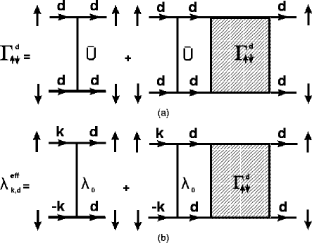
FIG. 2.: a) The vertex part of $\Gamma_{\uparrow\downarrow}^{d}$ in the ladder approximation. b) the corresponding vertex for the scattering of a pair of k-electrons into a pair of d-electrons.

To make contact with the Fermi-liquid picture of the Kondo problem, we rewrite this expression in the suggestive form

$$\frac{\Delta T_{c}}{T_{co}}\approx\frac{n_{s}}{\rho_{o}T_{K}}\ln\left(\frac{T_{K}}{T_{co}}\right)\left(2\eta-\ln\left(\frac{T_{K}}{T_{co}}\right)\right)$$ (26)

where we have used the fact that in the Kondo limit[21], $\pi\Gamma=\tilde{U}=4T_{K}/w$ with $w$ the Wilson number and we have dropped all irrelevant constants. Within the Fermi-liquid picture, $T_{c}\propto T_{K}\exp(\lambda^{-1})$ where $\lambda$ is the dimensionless phonon coupling. In this expression, $T_{K}$ replaces $\omega_{D}$ because electrons which are further away from the Fermi level than $T_{K}$ are strongly scattered. In the presence of $U$-impurities, there are two corrections to the dimensionless coupling constant $\lambda$. First, we must include the enhancement in the density of states arising from the Kondo resonance. This enhancement[7] scales as $n_{s}/T_{K}$. In addition, we must include the repulsion between quasiparticle states of opposite spin. The repulsion energy is essentially $T_{K}$ below the Kondo temperature[7, 21]. Within the quasi-particle picture, this repulsion is spread over $(\rho_{o}T_{K})^{2}$ states because there are two electrons participating in each scattering event. Hence, the change in the dimensionless coupling constant is given by[22]

$$\frac{\delta\lambda}{\lambda}=\frac{\delta\rho}{\rho_{0}}+\frac{\delta V}{V}=\frac{n_{s}}{\rho_{o}T_{K}}+\frac{n_{s}}{\lambda\rho_{o}T_{K}}$$ (27)

However, $\Delta T_{c}=-T_{c}\delta\lambda/\lambda^{2}$. Consequently, the initial slope in $T_{c}$ from the heuristic Fermi-liquid arguments

$$\frac{\Delta T_{c}}{T_{co}}=\frac{n_{s}}{\rho_{o}T_{K}}\ln\left(\frac{T_{K}}{T_{co}}\right)\left(1-\ln\left(\frac{T_{K}}{T_{co}}\right)\right)$$ (28)

is identical in form to the more exact expression derived in Eq. (26) because $\eta$ is $O(1)$. The second term in both of these expressions is the standard pair-weakening effect, whereas the first is a positive correction arising from the enhancement in the density of states at a Kondo impurity. In the strong-coupling regime, $|\lambda|>1$, Eq. (27) predicts that Kondo impurities can enhance $T_{c}$. We conclude then that non-magnetic impurities by virtue of local phonon pairing can counteract the standard $T_{c}$ suppressing effects and in some cases actually enhance $T_{c}$. Experimental systems on which this prediction can be tested are the transition metal alloy Ti(Fe) and degenerate semiconductors.

REFERENCES

[1] P. W. Anderson, Phys. Rev. 124, 41 (1961).
[2] M. J. Zuckermann, Phys. Rev. 140, A899 (1965).
[3]
C. F. Ratto and A. Blandin, Phys. Rev. 156, 513 (1967).
[4]
A. B. Kaiser, J. Phys. C. 3, 410 (1970).
[5]
J. Kondo, Prog. Theor. Phys. 32, 37 (1964).
[6]
K. Yosida, Phys. Rev. 147, 223 (1966).
[7]
P. Nozieres, J. Low Temp. Phys. 17, 31 (1974).
[8]
T. Matsuura, S. Ichinose, and Y. Nagaoka, Prog. Theor. Phys. 57, 713 (1977).
[9]
A. Sakurai, Phys. Rev. B 17, 1195 (1978).
[10]
N. E. Bickers and G. E. Zwicknagl, Phys. Rev. B 36, 6746 (1987).
[11]
L. S. Borkowski and P. J. Hirschfeld, J. Low Temp. Phys. 96, 185 (1994).
[12]
a.)H. Suhl, Low-Temperature Physics, lectures at Les Houches,
1961, edited by C. De Witt, B. Dreyfus, and P. G. de Gennes (Gordon and Breach, New York, 1962),
p. 258. b.) See also H. Suhl, D. R. Fredkin, J. S. Langer, and B. T. Matthias,
Phys. Rev. Lett. 9, 63 (1962).
[13]
D. Belitz, Phys. Rev. B 36, 47 (1987).
[14]
Y. Yosida, Prog. Theor. Phys. Suppl. 46, 244 (1970).
[15]
M. Salomaa, Solid State Comm. 38, 815 (1981); B. Horvatic and V. Zlatic,
ibid. 54, 957 (1985).
[16]
L. P. Gor’kov, Sov. Phys. JETP 2, 1364 (1959).
[17]
B. T. Matthias, A. C. Compton, H. Suhl, and E. Corenzwit, Phys. Rev. 115, 1597
(1959).
[18]
P. W. Anderson, Rev. Mod. Phys. 50, 191 (1978).
[19] I. A. Chernik and S. N. Lykov, Sov. Phys. Solid state 23,
1724 (1981); G. S. Bushmarina, I. A. Drabkin, V. V. Kompaniets, R. V., Parfen’ev,
D. V. Shamshur, and M. A. Shakhov, Sov. Phys. Solid State 28, 612 (1986).
[20]A. L. Shelankov, Solid State Comm. 62, 327 (1987).
[21]
A. C. Hewson, The Kondo Problem to Heavy Fermions (Cambridge University
Press, 1993), Chaps. 5 and 10.