[

Diffusion in a Random Velocity Field: Spectral Properties of a Non-Hermitian Fokker-Planck Operator

Abstract

We study spectral properties of the Fokker-Planck operator that describes particles diffusing in a quenched random velocity field. This random operator is non-Hermitian and has eigenvalues occupying a finite area in the complex plane. We calculate the eigenvalue density and averaged one-particle Green’s function, for weak disorder and dimension $d>2$. We relate our results to the time-evolution of particle density, and compare them with numerical simulations.

]

In contrast to closed quantum systems, classical systems often have dynamics generated by non-Hermitian operators. In this paper we develop general techniques to study the spectral properties of random non-Hermitian operators, and apply them to the Fokker-Planck (FP) operator that describes diffusion and advection of classical particles in a spatially random but time-independent velocity field:

$${\partial_{t}n}={{\cal L}_{fp}}n\equiv D\nabla^{2}n-{\nabla}\cdot({{\bf{V}}}n),$$ (1)

where $n$ is the concentration of particles, $D$ the molecular diffusivity, and ${\bf{V}}$ the background velocity field. The non-Hermitian character, in this case, is due to the advection term.

The statistical behavior of the scalar field $n$ obeying this FP equation has been investigated over a long history [1, 2, 3, 4], in the context of turbulent diffusion and anomolous diffusion in random media. However, for general velocity distributions, little appears to be known about spectral properties of the FP operator, such as the density of eigenvalues (DOS). An exception is the special case of potential flow, with ${\bf{V}}=\nabla\phi$. In this instance, there is a similarity transformation which maps the FP equation exactly to a Schrödinger equation in imaginary time[5]. The eigenvalues of the FP operator with potential flow are therefore real and negative. In one dimension, it is possible to express any velocity field in terms of a potential and to transform the FP equation in this way. Moreover, anomolous diffusion in one-dimensional systems with random flow has been shown to be connected with logarithmic singularities of the DOS and of the eigenstate localization length as the eigenvalue approaches zero [6]. In two dimensions, in the opposite case of incompressible flow ($\nabla.{\bf{V}}=0$), for which there is no similarity transformation to a Hermitian operator, localization of eigenfunctions of the FP operator has been studied numerically [7]. In addition, an analogy between the classical FP equation and the quantum random flux problem has been analyzed [7].

In general, the eigenvalues of a non-Hermitian FP operator occupy a finite area in the complex plane, rather than being restricted to the real-axis. This fact, despite the similarities in other respects between the FP and the Schrödinger equations, renders inapplicable [8] the standard perturbation expansion of Green’s functions, used for disordered quantum problems. Furthermore, saddle-point techniques [8, 9] developed for non-Hermitian random matrix ensembles [10, 11] are too specialized to be appropriate for random FP operators.

Very recently there has been considerable interest in properties of random non-Hermitian operators [12, 13, 14, 15], with a range of motivations, including the study of open quantum systems [9] and the motion of flux lines in superconductors[12]. Against this background, a better understanding of their spectral properties and of calculational methods is clearly desirable.

In this paper we describe a general scheme, based on a diagrammatic expansion, to compute the disorder-averaged Green’s functions and the DOS of random non-Hermitian operators. Similar ideas have been proposed in the context of random matrix theory by Feinberg and Zee [15]. We apply the technique to the FP operator of Eq.(1), calculating the shape of the support of the DOS, and the eigenvalue density itself. We also compare our analytical results with numerical calculations.

The particular FP operator we consider has constant diffusivity $D$ and a quenched random velocity field ${\bf{V}}({\bf{x}})$. Note that this is the opposite limit to that in the model recently discussed by Kraichnan [4], which has infinitely short time correlation in velocities. Time-independent flows can be established in physical systems such as porous media[3].

We take the velocity field to be gaussian distributed, with zero mean, and variance

$$\langle{\bf{V}}_{\alpha}({\bf{k}}){\bf{V}}_{\beta}({\bf{k}}^{\prime})\rangle = \Gamma_{1}(\delta_{\alpha\beta}-\frac{k_{\alpha}k_{\beta}}{{\bf{k}}^{2}})\delta({\bf{k}}+{\bf{k}}^{\prime})$$ (2)

$$+ \Gamma_{2}(\frac{k_{\alpha}k_{\beta}}{{\bf{k}}^{2}})\delta({\bf{k}}+{\bf{k}}^{\prime}),$$ (3)

where ${\bf{V}}({\bf{k}})=(2\pi)^{-d}\int d^{d}xe^{-i{\bf{k}}.{\bf{x}}}{\bf{V}}({\bf{x}})$, angular brackets denote the ensemble average, and $\Gamma_{1}$ and $\Gamma_{2}$ represent the strengths of the transverse and longitudinal parts of the velocity field. We take the spectrum of velocity fluctuations to have a short-wavelength cut-off, $\Lambda$, and consider a system of volume $\Omega$. The special case of mixed flow, $\Gamma_{1}=\Gamma_{2}=\Gamma$, leads to substantial simplifications: for clarity of presentation, we describe calculations only in this limit, but state results for the general problem.

At a complex frequency $\omega$, the dimensionless combination $\gamma(\omega)=(\Gamma/|\omega|^{2})(|\omega|/D)^{d/2+1}$ is a measure of the disorder strength. The fact that, as $\omega\to 0$, $\gamma(\omega)\to 0$ for $d>2$ and $\gamma(\omega)\to\infty$ for $d<2$, identifies $d=2$ as the upper critical dimension [3].

Our aim is to study spectral properties of the FP operator, ${\cal L}_{fp}$. We do so via the ensemble-averaged Green’s function

$$g(\omega)=\langle\frac{1}{\omega-{\cal L}_{fp}}\rangle.$$ (4)

Let $\langle L_{\lambda}|$ and $|R_{\lambda}\rangle$ be left and right eigenvectors of ${\cal L}_{fp}$ with eigenvalue $\lambda$, and let $|{\bf{p}}\rangle$ denote a plane-wave basis state with wavevector ${\bf{p}}$. The ensemble-averaged spectral density

$$C({\bf{p}},\omega)=\langle\sum_{\lambda}\langle{\bf{p}}|R_{\lambda}\rangle\langle L_{\lambda}|{\bf{p}}\rangle\delta(\omega-\lambda)\rangle$$ (5)

is diagonal in this basis, because averaging restores translational invariance. From it we can obtain the time Green’s function, or particle density, $\langle n({\bf{r}},t)\rangle$, evolving according to Eq (1) with initial condition $n({\bf{r}},t=0)=\delta({\bf{r}})$:

$$\langle n({\bf{r}},t)\rangle=(2\pi)^{-d}\int d^{d}{\bf{p}}\,e^{i{\bf{p}}.{\bf{r}}}\int d^{2}\omega\,e^{\omega t}C({\bf{p}},\omega)\,.$$ (6)

In the same basis, the diagonal elements of $g(\omega)$, which we compute, are related to $C({\bf{p}},\omega)$ by

$$g^{p}(\omega)=\int d^{2}\lambda\frac{C({\bf{p}},\lambda)}{\omega-\lambda}\,.$$ (7)

Analytic properties of the Green’s function depend on the eigenvalue density, $\rho(\lambda)$, in the complex $\lambda$-plane. In particular,

$$\rho(\omega)=\frac{1}{\pi}\frac{\partial}{\partial\omega^{*}}\frac{1}{\Omega}Trg(\omega)\,.$$ (8)

Thus, in the complex $\omega$-plane, $g(\omega)$ is non-analytic everywhere that the eigenvalue density is non-zero. Standard techniques for calculating disorder-averaged Green’s functions via perturbation theory yield only the part of $g(\omega)$ that is analytic in $\omega$, together with its analytic continuation inside the support of $\rho(\omega)$ [8]. In the special case of pure potential flow, $(\Gamma_{1}=0)$, the eigenvalues of ${\cal L}_{fp}$ all lie on the negative real axis and $g(\omega)$ is analytic elsewhere. Under these circumstances one can compute, for example, $\rho(\omega)$, in the usual way, from the discontinuity in $g(\omega)$ across the real axis. By contrast, for mixed flow (as we shall show), the eigenvalues of ${\cal L}_{fp}$ fill a finite area in the complex plane, the analytic part of $g(\omega)$ contains limited information, and a new approach is required.

To this end, for a general ${\cal L}$, we construct an matrix $\cal{H}$ which: (i) has twice the dimension of ${\cal L}$; (ii) is Hermitian; and (iii) has an inverse that contains $g(\omega)$ as one of four blocks. Specifically, with $A\equiv\omega-\cal{L}$,

$$\cal{H}=\left(\begin{array}[]{cc}\epsilon\hskip 14.22636ptA\\ A^{\dagger}\hskip 14.22636pt-1\\ \end{array}\right).$$ (9)

The inverse, $G\equiv{\cal H}^{-1}$, exists for real $\epsilon>0$ and is

$$G \equiv \left(\begin{array}[]{c}G_{11}\hskip 14.22636ptG_{12}\\ G_{21}\hskip 14.22636ptG_{22}\\ \end{array}\right)$$ (12)

$$= \left(\begin{array}[]{c}(\epsilon+AA^{\dagger})^{-1}\hskip 14.22636ptA(\epsilon+A^{\dagger}A)^{-1}\\ A^{\dagger}(\epsilon+AA^{\dagger})^{-1}\hskip 14.22636pt-\epsilon(\epsilon+A^{\dagger}A)^{-1}\\ \end{array}\right).$$ (15)

Since ${\cal H}$ is Hermitian, $G$ can be calculated using established methods, and from it we can obtain

$$g(\omega)=\lim_{\epsilon\rightarrow 0}\langle G_{21}\rangle.$$ (16)

This approach parallels recent work by Feinberg and Zee [15] and is somewhat different from that taken in other calculations on spectral properties of non-Hermitian operators: in the present notation, Sommers and collaborators [8, 13] focus on $\det(G_{11})$, while Efetov [14] separates ${\cal L}$ into Hermitian and anti-Hermitian parts.

A diagrammatic expansion for $\langle G\rangle$, and hence $g(\omega)$, follows from writing

$${\cal H}={\cal H}_{0}+{\cal H}_{1}\ ,$$ (17)

where

$${\cal H}_{0}=\left(\begin{array}[]{cc}\epsilon\hskip 14.22636pt0\\ 0\hskip 14.22636pt-1\\ \end{array}\right)\hskip 5.69046pt\mbox{and}\hskip 5.69046pt{\cal H}_{1}=\left(\begin{array}[]{cc}0\hskip 14.22636ptA\\ A^{\dagger}\hskip 14.22636pt0\\ \end{array}\right).$$ (18)

The series for $G$, in powers of ${\cal H}_{1}$ and of $G^{(0)}\equiv{\cal H}_{0}^{-1}$, involves two propagators, $G^{(0)}_{11}$ and $G^{(0)}_{22}$, and two vertices, $A$ and $A^{\dagger}$. As usual, it is convenient to introduce a self-energy, $\Sigma$, and proceed via the Dyson equation,

$$\langle G\rangle=G_{0}+G_{0}\Sigma\langle G\rangle,$$ (19)

where

$$G_{0}=\left(\begin{array}[]{c}1/\epsilon\hskip 14.22636pt0\\ 0\hskip 14.22636pt-1\end{array}\right).$$ (20)

To illustrate the approach, we consider first the asymmetric gaussian random matrix ensemble of Ref [8]: the $N\times N$ real matrix $[J]$ has the distribution $P[J]\propto exp(-NTr(JJ^{T}-\tau JJ)/[2(1-\tau^{2})])$ so that non-zero covariances are

$$<J^{T}_{ik}J_{ki}>=1/N,\hskip 14.22636pt<J_{ik}J_{ki}>=\tau/N.$$ (21)

The fully asymmetric problem, in which $\tau=1$ and $J_{ik}$ and $J_{ki}$ are statistically independent, was first studied by Ginibre [10], and has been treated using a Green’s function methods in Ref [15].

Setting ${\cal L}=J$, the leading contribution to the self energy at large $N$ comes from the diagrams of the self-consistent Born approximation (SCBA), shown in Fig 1.

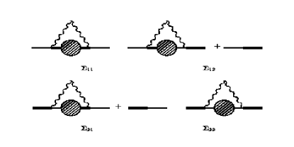
FIG. 1.: Self-energy diagrams in the SCBA. Single and double lines denote the two components of the bare $G_{0}$: $1/\epsilon$ and $-1$, respectively, while the internal digrams describe the four full Green’s functions.

From these we obtain

$$\Sigma=\left(\begin{array}[]{c}\langle G_{22}\rangle\hskip 14.22636pt\tau\langle G_{21}\rangle-\omega\\ \tau\langle G_{12}\rangle-\omega^{*}\hskip 14.22636pt\langle G_{11}\rangle\\ \end{array}\right).$$ (22)

Solving eq.(19), we recover the results of Ref [8]. In particular, inside the support of the $\rho(\omega)$, defined by $[x/(1+\tau)]^{2}+[y/(1-\tau)]^{2}<1$, we find

$$N^{-1}Trg(\omega)=(\frac{x}{1+\tau}-\frac{iy}{1-\tau}),\hskip 14.22636pt\omega=x+iy,$$ (23)

and hence a constant DOS, $\rho(\omega)=[\pi(1-\tau^{2})]^{-1}$.

With this preparation, we return to the Fokker-Planck operator of Eqs (1) and (3), taking $\Gamma_{1}=\Gamma_{2}\equiv\Gamma$. We find, at weak disorder and for dimension $d>2$, that the self-energy is again given by the SCBA. Corrections are small by a factor of the dimensionless disorder strength, $\gamma(x)$; neglecting these, we obtain the self-energy (diagonal in wavevector, $p$)

$$\Sigma_{p}=\left(\begin{array}[]{c}p^{2}\Gamma\int d^{d}{\bf{q}}\langle G^{q}_{22}\rangle\hskip 56.9055pt-\omega_{p}\\ -\omega_{p}^{*}\hskip 56.9055pt\Gamma\int d^{d}{\bf{q}}q^{2}\langle G^{q}_{11}\rangle\\ \end{array}\right),$$ (24)

where $\omega_{p}=\omega+Dp^{2}$.

Before discussing the self-consistent solution to Eqs (19) and (24), we note that one can arrive at the same point by expressing $G$ in terms of a functional integral, averaging using replicas, and making a simple decoupling approximation. In view of the $2\times 2$ block structure of $G$, it is natural to introduce two complex fields, $\eta_{1}$ and $\eta_{2}$, with $\eta^{\dagger}=(\eta_{1}^{\dagger},\eta_{2}^{\dagger})$, and write for $j,k=1$ or $2$

$$G_{jk}=i\langle Z^{-1}\int{\cal D}[\eta]\eta_{j}\eta_{k}e^{-iS}\rangle\,,$$ (25)

where the normalisation and action are

$$Z=\int{\cal D}[\eta]e^{-iS}\hskip 5.69046pt\mbox{and}\hskip 5.69046ptS=\eta^{\dagger}{\cal H}\eta\ .$$ (26)

The average over the velocity field, denoted by $\langle\ldots\rangle$ generates terms in the action of the form $\eta_{1,\alpha}^{\dagger}\eta_{1,\beta}\eta_{2,\beta}^{\dagger}\eta_{2,\alpha}$, where $\alpha$ and $\beta$ label replicas. Approximating these by setting

$$\eta^{\dagger}\eta\,\eta^{\dagger}\eta\approx\langle\eta^{\dagger}\eta\rangle\eta^{\dagger}\eta+\eta^{\dagger}\eta\langle\eta^{\dagger}\eta\rangle$$ (27)

we arrive at

$$G_{ik}=i\int{\cal D}[\eta]\eta_{i,\alpha}\eta_{k,\alpha}e^{-i{\tilde{S}}},$$ (28)

with ${\tilde{S}}=[G^{0}]^{-1}-\Sigma$, where $\Sigma$ is again given by Eq 24.

Proceeding now to the evaluation of the self-energy, we find

$$\langle G_{11}^{p}\rangle = \frac{1+F_{2}}{|\omega_{p}|^{2}+B_{p}},\hskip 8.5359pt\langle G_{12}^{p}\rangle=\frac{\omega_{p}}{|\omega_{p}|^{2}+B_{p}}$$ (29)

$$\langle G_{21}^{p}\rangle = \frac{\omega_{p}^{*}}{|\omega_{p}|^{2}+B_{p}},\hskip 8.5359pt\langle G_{22}^{p}\rangle=-\frac{\epsilon+p^{2}F_{1}}{|\omega_{p}|^{2}+B_{p}}\,,$$ (30)

where $B_{p}=(\epsilon+F_{1})(1+F_{2})$ and

$$F_{1}=-\Gamma\int_{0}^{\Lambda}d^{d}{\bf{q}}\langle G_{22}^{q}\rangle,\hskip 8.5359ptF_{2}=\Gamma\int_{0}^{\Lambda}d^{d}{\bf{q}}\,q^{2}\langle G_{11}^{q}\rangle.$$ (31)

Analysing this system of equations in the limit $\epsilon\to 0$, we obtain

$$g^{p}(\omega)=\frac{\omega_{p}^{*}}{|\omega_{p}|^{2}+bp^{2}}\,.$$ (32)

where the value of $b$ is determined via behaviour of the integral

$$I(b)=\Gamma\int_{0}^{\Lambda}d^{d}{\bf{q}}\frac{q^{2}}{|\omega_{q}|^{2}+bq^{2}}.$$ (33)

If $I(b=0)<1$, then $b=0$; otherwise $b$ is the (real and positive) solution to the equation $I(b)=1$. The former is the case if $\omega$ is not close to the negative real axis. In that event, with $b=0$, $g^{p}(\omega)=\omega_{p}^{-1}$ and $\partial g^{p}(\omega)/\partial\omega^{*}=0$, so that $\rho(\omega)=0$. Alternatively, if $\omega$ is close to the negative real axis, $b>0$, $g^{p}(\omega)$ is not analytic in $\omega$ and $\rho(\omega)\not=0$.

Thus the boundary to the support of the density of states, $y_{B}(x)$, satisfies the equation

$$I(b=0)\equiv\Gamma\int_{0}^{\Lambda}d^{d}{\bf{q}}\frac{q^{2}}{(x+Dq^{2})^{2}+y_{B}^{2}}=1.$$ (34)

For small $\Gamma$, $d>2$ and $x<0$, we find

$$y_{B}(x)=\pm\frac{\pi S_{d}}{2}\gamma(x)|x|\propto\pm\Gamma|x|^{d/2}$$ (35)

where $S_{d}$ is the surface area of a $d$-dimensional unit sphere. The DOS in the region $x<0,|y|<y_{B}$ is

$$\rho(\omega)=\frac{D}{(2\pi)^{d+1}\Gamma|x|}\,.$$ (36)

and elsewhere is zero. Thus the eigenvalues occupy a wedge-shaped region in the complex plane, centered around the negative real axis. The $x$-dependent width of this region can be understood simply: if one assumes that it is proportional to $\Gamma$, dimensional analysis implies $y_{B}(x)\propto\gamma(x)|x|$. Similarly, the $x$-dependence of $\rho(\omega)$ follows from the requirement that $\int dy\rho(x+iy)$ take the value it has in the disorder-free system.

Turning to the time-evolution of the particle density, we find that the time Green’s funtion, defined in Eq (6), is the Fourier transform of a product of two factors:

$$\langle n({\bf{r}},t)\rangle=\frac{1}{(2\pi)^{d}}\int d^{d}{\bf{p}}\,e^{i{\bf{p}}.{\bf{r}}}\,e^{-Dp^{2}t}\,[\frac{\sin(\omega_{0}t)}{\omega_{0}t}]\,,$$ (37)

where $\omega_{0}=y_{B}(x)$, evaluated at $x=-Dp^{2}$: $\omega_{0}=(\pi S_{d}\Gamma q^{d})/(2D)$. The first factor, $e^{-Dp^{2}t}$, is the familiar consequence of simple diffusion; the second factor, $\sin(\omega_{0}t)/\omega_{0}t$, arises from advection. At weak disorder, when the SCBA is a controlled approximation, the advective factor differs significantly from $1$ only where the diffusive factor is small, so that $\langle r^{2}\rangle\sim Dt$. By contrast, at strong disorder (when the SCBA is simply a mean-field approximation), it is the advective factor that sets the width of of the density profile at short times, and $\langle r^{2}\rangle\sim(\Gamma t/D)^{2/d}$. This time-dependence arises because advection and diffusion contribute equally to particle motion in this regime.

For general random flow, with $\Gamma_{1}\not=\Gamma_{2}$, an extension of our approach again yields Eqs (35), (36) and (37), but with $\Gamma_{1}$ replacing $\Gamma$. Thus, in particular, for potential flow ($\Gamma_{1}=0$) we reproduce correctly the fact that all eigenvalues are real.

To test the theory developed above, we have calculated numerically the eigenvalues of the FP operator for mixed flow, discretized on a square lattice. Theory (adapted to the discretized FP operator) and simulation are compared in Fig (2), for 50 realisations of a $32\times 32$ lattice with $D=1$ and $\Gamma=0.25$.

The calculated shape of the support of $\rho(\omega)$ matches the data well; the fact that a finite fraction of the eigenvalues have vanishing imaginary part is a finite-size effect, analyzed in detail in Ref[14].

J.T.C. is grateful to the Institute for Theoretical Physics, UCSB, for hospitality during completion of this work, which was supported by EPSRC grant GR/GO 2727, and by NSF grant PHY94-07194; Z.J.W. acknowleges the support by an EPSRC grant, and a NSF-NATO postdoctoral fellowship.

$\dagger$ Current address: Courant Institute of Mathematical Sciences, New York University, 251 Mercer St., New York, NY 10012. Electronic mail: jwang@cims.nyu.edu.

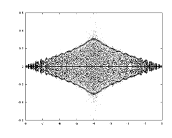
FIG. 2.: Distribution of eigenvalues (dots) in the complex plane, and calculated boundary ($\diamond$) of $\rho(\omega)$.

REFERENCES

- [1] For reviews, see: M. B. Isicheko, Rev. Mod. Phys., 64, 961 (1992), and J. P. Bouchaud and A. Georges, Phys. Rep. 195, 127 (1990).
- [2] Ia. Sinai, in Proceedings of the Berlin Conference in Mathematical problems in theoretical Physics, edited by R. Schrader et. al. (Springer, Berlin, 1982), p12.
- [3] D. S. Fisher, Phys. Rev. A 30, 960 (1984); D. S. Fisher, Z. Qiu, S. J. Shenker, and S. H. Shenker, ibid. 31, 3841 (1985); J. A. Aronovitz and D. R. Nelson, ibid. 30, 1948 (1984); V. E. Kravtsov, I. V. Lerner, and V. I. Yudson, J. Phys. A18, L703 (1985); Zh. Eksp. Teor. Fiz. 91, 569 (1996) [Sov. Phys. JETP 64, 336 (1986)]; Phys. Lett. A119, 203 (1986); I.V. Lerner, Nucl. Phys. A 560, 274 (1993).
- [4] R. H. Kraichnan, Phys. Rev. Lett. 72, 1016 (1994).
- [5] H. Risken, The Fokker-Planck Equation (Spring-Verlag, Berlin and Heidelberg, 1989).
- [6] S. Alexander, J. Bernasconi, W. R. Schneider, and R. Orbach, Rev. Mod. Phys. 53, 175 (1981); E. Tosatti, M. Zannetti, and L. Pietronero, Zeit. Phys. B 73, 161 (1988).
- [7] J. Miller and Z. J. Wang, Phys. Rev. Lett. 76, 1461 (1996).
- [8] H. J. Sommers, A. Crisanti, H. Sompolinsky, and Y. Stein, Phys. Rev. Lett. 60, 1895 (1988).
- [9] F. Hakke et al., Zeit. Phys. B 88, 359 (1992).
- [10] J. Ginibre, J. Math. Phys. 6, 440(1965), M. L. Mehta, Random Matrices (Academic Press Inc., Boston, 1990).
- [11] V. L. Girko, Theory Probab. Its Appl. (USSR) 29, 694 (1985).
- [12] N. Hatano and D. R. Nelson, Phys. Rev. Lett. 77, 570 (1996).
- [13] Y. V. Fyodorov, B. Khoruzhenko, and H.-J. Sommers, cond-mat/9606173, Y. V. Fyodorov, B. Khoruzhenko, and H.-J. Sommers, cond-mat/9702152.
- [14] K. B. Efetov, cond-mat/9702091.
- [15] J. Feinberg and A. Zee, hep-th/9703087