The Anderson transition: time reversal symmetry and universality

Abstract

We report a finite size scaling study of the Anderson transition. Different scaling functions and different values for the critical exponent have been found, consistent with the existence of the orthogonal and unitary universality classes which occur in the field theory description of the transition. The critical conductance distribution at the Anderson transition has also been investigated and different distributions for the orthogonal and unitary classes obtained.

It is now widely accepted that the metal- insulator transition for non- interacting electrons, the so called Anderson transition [1], is a continuous phase transition in which static disorder plays a role analogous to temperature in thermal phase transitions. The field theoretical formulation of the problem [2], though not making reliable predictions for the critical exponent [3, 4], does indicate that it should be possible to describe the critical behavior within a framework of three universality classes: orthogonal, unitary and symplectic. However, recent work put this idea in question. It was found that the scaling functions for systems with orthogonal and unitary symmetry could not be distinguished at an accuracy of a few percent [5]. Nor could the values of the critical exponent for the three universality classes be reliably distinguished [5, 6, 7, 8, 9]. This, together with recent work on the statistics of energy levels in the vicinity of transition, has prompted the suggestion [10] that the universality classes predicted by the field theory do not correctly describe the Anderson transition.

The two important symmetries in the field theory are time reversal symmetry (TRS) and spin rotation symmetry (SRS). The system is said to be in the orthogonal universality class if it has both SRS and TRS, in the unitary class if TRS is broken and in the symplectic class if the system has TRS but SRS is broken. The relevant terms in the Hamiltonian are a coupling to an applied magnetic field, which breaks TRS, and the spin orbit interaction, which breaks SRS.

Here we focus on the breaking of TRS by a constant applied magnetic field. We report the results of Monte Carlo studies which indicate that the critical behavior, at least as far as orthogonal and unitary symmetries are concerned, is in accord with the conventional universality classes. By carrying out a precise study of the finite size scaling of the electron localization length, which is analogous to the correlation length in thermal transitions, we have clearly differentiated the scaling functions for the orthogonal and unitary universality classes. We have also estimated the critical exponents and calculated confidence intervals for these estimates. We find a statistically significant difference of about $12\%$ between the values of the critical exponent in the orthogonal and unitary classes.

To reinforce the above conclusion we have also simulated the critical conductance distribution of a disordered mesoscopic conductor. Following the discovery of universal conductance fluctuations it was realized that the conductance of a phase coherent system is not self- averaging. Extrapolating from the metallic regime, it seems that the conductance fluctuations at the critical point should be of the same order of magnitude as the mean conductance and that the full conductance distribution should be a more useful characteristic of the critical point. As we approach the critical point the localization length diverges and the system becomes effectively self similar, we then expect the conductance distribution to become independent of system size and depend only on the universality class. This expectation was borne out in our study where we found different critical conductance distributions depending on whether or not TRS is broken.

The model Hamiltonian used in this study describes non- interacting electrons on a simple cubic lattice. With nearest neighbor interactions only we have

$$\begin{array}[]{lll}<\vec{r}|H|\vec{r}>&=&V(\vec{r}),\\ <\vec{r}|H|\vec{r}-\hat{x}>&=&1,\\ <\vec{r}|H|\vec{r}-\hat{y}>&=&1,\\ <\vec{r}|H|\vec{r}-\hat{z}>&=&\exp(-i2\pi\phi x),\end{array}$$ (1)

where $\hat{x}$, $\hat{y}$ and $\hat{z}$ are the basis vectors of the lattice. The electrons are subject to an external magnetic field applied in the $\hat{y}$ direction whose strength is parameterized by the flux $\phi$, measured in units of the flux quantum $h/e$, threading a lattice cell. The on site energies of the electrons $\{V(\vec{r})\}$ are assumed to be independently and identically distributed with probability $p(V)\text{d}V$ where

$\displaystyle\begin{array}[]{llll}p(V)&=&1/W&|V|\leq W/2,\\ &=&0&{\rm otherwise}.\end{array}$

The critical point, scaling function and the value of the critical exponent for several values of $\phi$ and Fermi energy $E_{f}$ (see Table I) are determined by examining the finite size scaling [11] of the localization length $\lambda$ for electrons on a quasi-$1d$ dimensional bar of cross section $L\times L$. The localization length $\lambda\equiv\lambda(E_{f},\phi,W,L)$, defined by

$$\lambda^{-1}=\lim_{L_{z}\rightarrow\infty}\frac{<-\ln g(L_{z})>}{2L_{z}},$$ (2)

where $L_{z}$ is the length of the bar and $g(L_{z})$ is the conductance of the bar measured in units of $(e^{2}/h)$, can be evaluated by rewriting the Schroedinger equation as a product of transfer matrices; $\lambda^{-1}$ can then be determined to within a specified accuracy using a standard technique [12]. The accuracy used here ranges between $0.1\%$ and $0.2\%$.

On intuitive grounds it has been argued [13] that we should observe orthogonal scaling when $L\ll L_{H}$ and unitary scaling when $L\gg L_{H}$ where $L_{H}$ is the magnetic length. For the lattice model (1) $L_{H}=\sqrt{1/2\pi\phi}$. For the smallest system size $L=6$ used here this criterion yields a crossover flux $\phi_{c}\simeq 1/226$. We thus expect to see clear unitary scaling behavior for cases Ua and Ub listed in Table I.

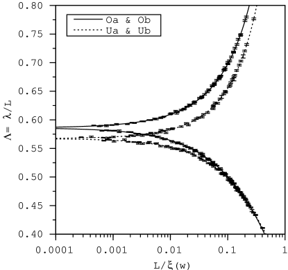
FIG. 1.: The scaling of the data for the parameter sets listed in Table I. The lines are the scaling functions given by (5) and (6). Different scaling functions for the orthogonal and unitary universality classes can be clearly distinguished.

When the dimensionless quantity $\Lambda=\lambda/L$ is plotted against disorder $W$ for different cross sections $L$ the curves are found to have a common point of intersection; this indicates the occurrence of the metal- insulator transition at a critical disorder $W_{c}$ in the $3d$ system which would be obtained by letting $L\rightarrow\infty$. Detailed analysis of the data is based on the following assumptions: first that for $L$ finite $\Lambda$ is a smooth function of $W$ and $L$, second that the data obey a one parameter scaling law

$$\Lambda(W,L)=f_{\pm}(L/\xi(w)),$$ (3)

where $w=(W_{c}-W)/W_{c}$ and the subscript $\pm$ refers to $w>0$ and $w<0$, and third that the length $\xi$ appearing in the scaling law has a power law divergence close to $W_{c}$ of the form $\xi(w)=\xi^{\pm}|w|^{-\nu}$. This relation defines the critical exponent $\nu$ and introduces two arbitrary constants $\xi^{+}$ $(w>0)$ and $\xi^{-}$ $(w<0)$. According to the Wegner scaling law [14] $\nu$ is related to the critical exponent $s$ associated with the conductivity by $s=(d-2)\nu$ so that $\nu=s$ in $d=3$. The above assumptions imply that it should be possible to fit the data to

$$\Lambda_{\text{fit}}(W,L)=\Lambda_{c}+\sum_{n=1}A_{n}L^{n/\nu}w^{n}.$$ (4)

In practice we have truncated this series at $n=3$. The relation between (3) and (4) can be made apparent by writing

$$\begin{array}[]{ll}f_{+}=\Lambda_{c}+\sum_{n=1}a_{n}\left(L/\xi\right)^{n/\nu},&a_{n}=A_{n}\left(\xi^{+}\right)^{n/\nu}\end{array},$$ (5)

$$\begin{array}[]{ll}f_{-}=\Lambda_{c}+\sum_{n=1}b_{n}\left(L/\xi\right)^{n/\nu},&b_{n}=(-1)^{n}A_{n}\left(\xi^{-}\right)^{n/\nu}\end{array}.$$ (6)

In principle $\xi^{+}$ and $\xi^{-}$ should depend on energy and flux though the “amplitude ratio” $\xi^{+}/\xi^{-}$ may be universal [15] so that $\xi^{+}$ and $\xi^{-}$ may not be independent. Their absolute values cannot be determined using the present method. No relative variation as a function of energy and flux, which would be apparent in the simulation, was detected. Therefore for convenience we set $\xi^{+}=\xi^{-}=1$. The most likely fit is determined by minimizing the $\chi^{2}$-statistic

$$\chi^{2}=\sum_{m}\left(\frac{\Lambda_{m}-\Lambda_{\text{fit}}(W_{m},L_{m})}{\sigma_{m}}\right)^{2},$$ (7)

where the summation $m$ is over all data points and $\sigma_{m}$ is the error (standard deviation) in the determination of the $m$th data point. After being fitted the data are re-plotted against $L/\xi$ to check that they obey the scaling law (3).

We also need to determine the goodness of fit $Q$ and confidence intervals for the fitting parameters. The goodness of fit measures the credibility of the fit; $Q>0.001$ is often regarded as acceptable in other applications [16]. We have checked that the numerical procedure used to estimate the localization lengths does so with an error which is approximately normally distributed. If we ignore the presence of any systematic corrections to scaling in the data, this permits the use of the $\chi^{2}$ likely-hood function to determine the “best fit” and the estimation of $Q$ from the $\chi^{2}$ distribution with $M-N$ degrees of freedom.

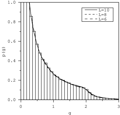
FIG. 2.: The critical conductance distributions for parameter set Oa listed in Table  I.

The confidence intervals for the fitted parameters were estimated in two independent ways: first from the Hessian matrix obtained in the least squares fitting procedure and second using the Bootstrap procedure described in [16]. In the latter method the original data are repeatedly randomly sampled (with replacement) and fitted. This provides an independent check of the distribution of the fitted parameters. Both methods gave approximately the same results. We chose to present the errors as $95.4\%$ marginal confidence intervals as given by the Boostrap method.

The results are summarized in Tables I and II. Given the confidence intervals the probability that the values of the critical exponent for the orthogonal and unitary universality classes are the same seems to be negligible. Different values of $\Lambda_{c}$ can also be distinguished confirming what is clearly evident in Fig. 1 that the orthogonal and unitary data scale differently. We conclude that the scaling function is sensitive to the breaking of time reversal symmetry.

We now turn to the conductance distribution. We consider a cubic “sample” of side $L$ attached to semi- infinite leads on two opposite faces. The disorder $W$ is set to zero in the leads, the Fermi energy and magnetic field are constant throughout. The zero temperature linear conductance $G=(e^{2}/h)g$ can be obtained from $g={\rm tr}tt^{\dagger}$ where $t$ is the transmission matrix of the sample. The $t$ matrix can be related to a Green’s function [17, 18] which can be determined iteratively.

For each set of parameters we have calculated the conductances for an ensemble of $100,000$ realizations of the random potential. Some typical results are presented in Fig. 2. Our analysis of these results is based on the generalization of (3) $p(g)=p(g,L/\xi)$. At the critical point $\xi$ diverges and we should obtain a universal critical conductance distribution $p_{c}(g)$ which is independent of $L$. The scale invariance of $p_{c}(g)$ is clearly demonstrated, at least for the range of system sizes studied, in Fig. 2. We found a similar scale invariance for all the cases listed in Table I. In Fig. 3 we have plotted the critical conductance distributions obtained and in Table III tabulated some averages of these distributions. The results are consistent with the existence of distinct orthogonal and unitary critical conductance distributions.

We now discuss the general features of $p_{c}(g)$ focusing on the orthogonal universality class and making a comparison with the critical distribution obtained in the $\epsilon$ expansion in the field theory. The $n$th cumulant $c_{n}$ of $p_{c}(g)$ for a $d$ dimensional cube of linear dimension $L$ is [19]

$$\begin{array}[]{ll}c_{n}=\left(\frac{\pi}{2}\right)^{n}&\left\{\begin{array}[]{ll}\epsilon^{n-2}&n\lesssim n_{0}\\ (L/l)^{\epsilon n^{2}-2n}&n\gtrsim n_{0}\end{array}\right.\end{array}$$ (8)

where $\epsilon=d-2$, $n_{0}$ is an integer of order $1/\epsilon$ and $l$ is the elastic mean free path. As described in [20] it is possible, under certain assumptions, to derive $p_{c}(g)$ from this. Extrapolating to $d=3$ we find

$$p_{\epsilon}(g)=\frac{1}{{\rm e}}\delta(g)+\frac{\pi}{2\text{e}}\left(u(\frac{\pi g}{2})+\frac{1}{2!}[u*u](\frac{\pi g}{2})+\dots\right),$$ (9)

where $u(x)=4x^{-3}\exp(-2/x)$, $*$ denotes the convolution and e=2.71828… The series (9) is easily handled numerically. The result is shown in Fig. 3.

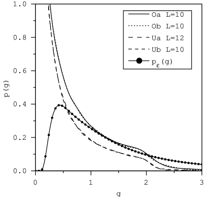
FIG. 3.: The distribution of $g$ at the critical point. Orthogonal and unitary distributions can be clearly distinguished. The critical conductance distribution obtained in the $\epsilon$ expansion is also shown.

The most obvious feature is that $p_{c}(g)$ is not peaked about its mean value $<g>$. The conductance fluctuations, as measured by the standard deviation $\sigma_{g}$, are of the same order of magnitude as $<g>$. If we compare with $p_{\epsilon}(g)$ we find that we have a good approximation to the central region of the distribution function but a rather bad approximation to its tails. The large $g$ tail of $p_{\epsilon}(g)$ decays as $1/g^{3}$ which means that all cumulants higher than $c_{1}$ diverge. This is reflected in (8) where these cumulants are not universal but depend on $l$ and $L$. We could find no evidence of this behavior, however, in the simulation; as seen in Fig. 3 there is sharp decay of $p_{c}(g)$ above $g\simeq 2$ and the higher cumulants, at least as far as $n=4$, seem to have universal values.

Another way to look at the critical distribution is to change variables to $\ln g$ (see Fig. 4). While the distribution is certainly not of Gaussian form, it does show a central tendency.

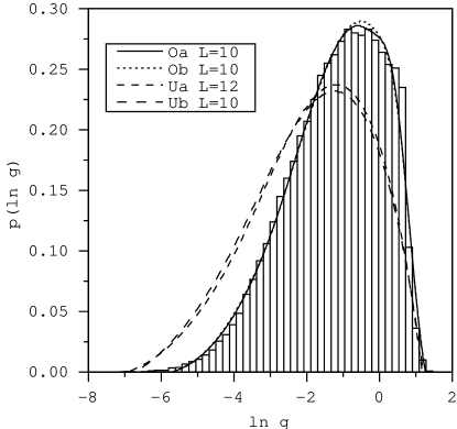
FIG. 4.: The critical distribution after changing variables.

In conclusion we have presented numerical evidence which, we think, confirms that the critical behavior at the Anderson transition is sensitive to perturbations which break time reversal symmetry.

T.O. would like to thank Yoshiyuki Ono for important discussions at the outset of the present work. Some of this work was carried out on supercomputer facilities at the ISSP, Univ. Tokyo and the Institute of Physical and Chemical Research.

Label	$E_{f}$	$\phi$	$L$	$[W_{min},W_{max}]$	$M$	$N$	$\chi^{2}_{\text{min}}$	Q
Oa	$0$	$0$	$\{6,8,10,12\}$	$[15,18]$	$86$	$6$	$79$	0.50
Ob	$0.5$	$0$	$\{6,8,10\}$	$[15.6,17.6]$	$73$	$6$	$49$	0.96
Ua	$0$	$1/3$	$\{6,9,12\}$	$[17,20]$	$55$	$6$	$35$	0.94
Ub	$0$	$1/4$	$\{8,10,12,14\}$	$[17.5,19.5]$	$66$	$6$	$65$	0.31

TABLE I.: The parameters used in the numerical study: Fermi energy $E_{f}$, flux $\phi$, system sizes $L$, the range of disorder, the number of data points $M$, the number of fitting parameters $N$, the value of $\chi^{2}$ for the best fit $\chi^{2}_{\text{min}}$ and the goodness of fit Q as estimated from the $\chi^{2}$ distribution.

Label	$W_{c}$	$\Lambda_{c}$	$\nu$
Oa	$16.448\pm.014$	$0.5857\pm.0012$	$1.59\pm.03$
Ob	$16.442\pm.018$	$0.5862\pm.0015$	$1.60\pm.06$
Ua	$18.316\pm.015$	$0.5683\pm.0013$	$1.43\pm.04$
Ub	$18.375\pm.017$	$0.5662\pm.0016$	$1.43\pm.06$

TABLE II.: The best fit values of the critical parameters together with their $95.4\%$ confidence intervals as estimated using the bootstrap method.

Label	$<g>$	$\sigma_{g}$	$<\ln g>$	$\sigma_{\ln g}$
Oa $L=10$	$0.579$	$0.598$	$-1.206$	$1.319$
Ob $L=10$	$0.578$	$0.598$	$-1.207$	$1.318$
Ua $L=12$	$0.395$	$0.499$	$-1.869$	$1.590$
Ub $L=10$	$0.395$	$0.499$	$-1.864$	$1.583$

TABLE III.: The means and standard deviations of the critical distribution of $g$ and $\ln g$.

REFERENCES

- [1] For a review see B. Kramer and A. MacKinnon, Rep. Prog. Phys. 56, 1469 (1993).
- [2] K. B. Efetov, Adv. in Phys. 32, 53 (1983).
- [3] W. Benreuther and F. Wegner, Phys. Rev. Lett. 57, 1385 (1986).
- [4] S. Hikami, Prog. Theo. Phys. Supp. 107, 213 (1992).
- [5] M. Henneke, B. Kramer and T. Ohtsuki, Europhys. Lett. 27, 389 (1994).
- [6] A. MacKinnon, J. Phys.: Condens. Matt. 6, 2511 (1994).
- [7] T. Ohtsuki, B. Kramer and Y. Ono, J. Phys. Soc. Jpn. 62, 224 (1993).
- [8] J.T. Chalker and A. Dohmen, Phys. Rev. Lett. 75, 4496 (1995).
- [9] T. Kawarabayashi, T. Ohtsuki, K. Slevin and Y. Ono, Phys. Rev. Lett. 77, 3593 (1996).
- [10] E. Hofstetter, cond-mat/9611060.
- [11] Ch. 9, Lectures on Phase Transitions and the Renormalization Group, N. Goldenfeld (Addison Wesley, 1992).
- [12] A. MacKinnon and B. Kramer, Z. Phys. B 53, 1 (1983).
- [13] I. Lerner and Y. Imry, Europhys. Lett. 29, 49 (1995).
- [14] F. Wegner, Z. Phys. B 25, 327 (1976).
- [15] Ch. 28, Quantum Field Theory and Critical Phenomena J. Zinn-Justin (Oxford, 1996).
- [16] Ch. 15, Numerical Recipes in Fortran, W. Press, B. Flannery and S. Teukolsky, (Cambridge Univ. Press, 1992).
- [17] Ch. 3, Electronic Transport in Mesoscopic Systems S. Datta (Cambridge Univ. Press, 1995).
- [18] T. Ando, Phys. Rev. B 44, 8017 (1991).
- [19] B.L. Altshuler, V. Kravtsov and I. Lerner, Sov. Phys. JETP 64, 1352 (1986); Phys. Lett. A134, 488 (1989).
- [20] B. Shapiro, Phys. Rev. Lett. 65, 1510 (1990); A. Cohen and B. Shapiro, Int. J. Mod. Phys. B6, 1243 (1992)